HAL Id: hal-01320003
https://hal.archives-ouvertes.fr/hal-01320003
Submitted on 13 Nov 2019
HAL is a multi-disciplinary open access
archive for the deposit and dissemination of
sci-entific research documents, whether they are
pub-lished or not. The documents may come from
teaching and research institutions in France or
abroad, or from public or private research centers.
L’archive ouverte pluridisciplinaire HAL, est
destinée au dépôt et à la diffusion de documents
scientifiques de niveau recherche, publiés ou non,
émanant des établissements d’enseignement et de
recherche français ou étrangers, des laboratoires
publics ou privés.
Representation and Processing
Jiří Havel, François Merciol, Sébastien Lefèvre
To cite this version:
Jiří Havel, François Merciol, Sébastien Lefèvre. Efficient Tree Construction for Multiscale Image
Representation and Processing.
Journal of Real-Time Image Processing, Springer Verlag, 2016,
�10.1007/s11554-016-0604-0�. �hal-01320003�
Jiˇr´ı Havel · Fran¸cois Merciol · S´ebastien Lef`evre
Efficient Tree Construction for Multiscale Image
Representation and Processing
Received: date / Revised: date
Abstract With the continuous growth of sensor perfor-mances, image analysis and processing algorithms have to cope with larger and larger data volumes. Besides, the informative components of an image might not be the pixels themselves, but rather the objects they belong to. This has led to a wide range of successful multiscale techniques in image analysis and computer vision. Hi-erarchical representations are thus of first importance, and require efficient algorithms to be computed in or-der to address real-life applications. Among these hier-archical models, we focus on morphological trees (e.g., min/max-tree, tree of shape, binary partition tree, α-tree) that come with interesting properties and already led to appropriate techniques for image processing and analysis, with a growing interest from the image pro-cessing community. More precisely, we build upon two recent algorithms for efficient α-tree computation and introduce several improvements to achieve higher perfor-mance. We also discuss the impact of the data structure underlying the tree representation, and provide for the sake of illustration several applications where efficient multiscale image representation leads to fast but accu-rate techniques, e.g. in remote sensing image analysis or video segmentation.
1 Introduction
Mathematical morphology has long been a provider of interesting hierarchical image representations, mainly by trees, e.g., component tree [22], min and max-tree [35], binary partition tree [34], etc. The max-tree (and its re-spective counterpart, min-tree) has been widely used due J. Havel
Brno University of Technology, Czech Republic Tel.: +420 54114-1474
Fax: +420 54114-1270 E-mail: [email protected] F. Merciol, S. Lef`evre
Universit´e de Bretagne-Sud, IRISA, France
E-mail: {francois.merciol,sebastien.lefevre}@univ-ubs.fr
to its nice properties as well as the availability of efficient algorithms to first compute the tree from an image, and second process the tree (e.g., with a filtering to remove irrelevant nodes), thus leading to the processing of the underlying image.
The min and max-tree can be combined together to form a tree of shapes [42]. In the tree of shapes, child nodes represent parts of a larger object. Another im-provement of min/max-trees uses second generation con-nectivity [28], where the contents of the tree and its shape are defined by two independent images.
Recently, a new image model, namely the α-tree [29], has been introduced to avoid relying on an ordering re-lation among image pixels. This model is a hierarchical representation of the quasi-flat zones of an image, and as such, relies on local dissimilarities α. This model already led to successful attempts in exploration of remote sens-ing data [27] and image/video segmentation [19]. Due to the locality of the α-tree, an (α, ω)-tree was introduced [39, 40]. (α, ω)-tree uses nonlocal infomations to prevent forming of excessively large components.
There is large amount of algorithms for construction of min/max-tree [7]. For α-tree construction, two algo-rithms have been recently introduced. One [12] focuses mainly on utilizing parallelism on modern multicore pro-cessor. The other [23] is based on relationship [9] of var-ious trees (binary partition tree by altitude ordering, α-tree, min/max-α-tree, wathersheds, ...) to the minimum spanning tree. In this paper, we fuse these approaches. Additionally, the relationship of min/max-tree and the minimum spanning tree will be slightly extended to in-clude mask based second generation connectivity.
Section 2 will briefly describe various component trees and their relationship. Section 3 compares some possible representations of the component tree and describes the combined algorithm for construction of α-tree. In sec-tion 4, all algorithms are compared in terms of perfor-mance and section 5 illustrate the relevance of α-tree with various applications facing large data volume.
2 Connected Component Trees 2.1 Definitions
All connected component trees represent an image as a hierarchy of regions i.e., connected sets of pixels. For the purpose of the connected component trees, the image is a undirected graph G = (V, E, I), where the vertices V correspond to the image pixels (so either V ⊂Z2, or an
injective mapping pixel : V → Z2 can be constructed)
and the edges E connect pixels as described by the inci-dence relation I ⊆ V × E. For the purpose of this paper, the sets V and E are some identifiers of vertices and edges, so the sets are disjoint. The exact nature of these identifiers is not important. We will also disallow hyper-graphs (and loops) (∀e ∈ E : |{v ∈ V | vIe}| = 2) and multigraphs (∀v1, v2 ∈ V : |{e ∈ E | v1Ie, v2Ie}| ≤ 1).
This definition allows to make subgraphs by subsetting V and E and keeping I intact. The degree of vertices de-pends on the image connectivity. For square pixels and grid, 4- or 8-connectivity is most common. 6-connectivity is sometimes used, but is typical for hexagonal pixels and grid. The degree of a vertex (with the exception of image border) is equal to the image connectivity.
A connected component tree (CCT) is a rooted tree whose each node corresponds to a connected component (CC). A CC is a subgraph whose all vertices are all con-nected by a path and no additional vertex can be added to it. To get a hierarchical tree and not only a single partition, CCT must contain CCs of various image sub-graphs Gi = (Vi ⊆ V, Ei ⊆ E, I), or shortly Gi ⊆ G.
Additionally, a tree node (i.e., a subgraph of G) must in-clude the union of all its children. Usually, only the tree root is a CC of G (usually the whole image).
The hierarchy of subgraphs can be created by intro-ducing a weight function w : V + E → W , that assigns weights to all vertices and edges of the image graph. The weight functions for vertices and edges can be different and the weight sets too, but we use only one for the sake of simplicity. The set of weights W is usually a subset of R and must have total ordering. A set of CCs for a
weight wi∈ W is a set of CCs of subgraph Gi:
Vi= {v ∈ V | w(v) ≤ wi} (1)
Ei= {e ∈ E | w(e) ≤ wi} (2)
These CCs form a level of the CCT that corresponds to the weight wiand contain subsets of vertices and edges of
G. For simplicity, we will write that these CCs and the tree level have the weight wi. A vertex v first appears
in the tree level with weight w(v) and is present in all parent levels all the way to the root.
A CCT can provide a hierarchy of image segmen-tations. A segmentation is a decomposition of an im-age into disjoint groups of pixels (segments or regions), whose union is the complete image. To provide a seg-mentation, the tree must contain all image pixels at the
level min(W ). If a tree has vertices at a different level, the segmentation can be constructed by setting w(v) = min(W ), i.e. by pulling the pixels as separate leaves. Such segmentation adds single-pixel segments for all vertices that appear on a level closer to the root.
Cousty et. al. [9] have shown, that the edge weights alone are sufficient for construction of various morpho-logical trees such as
– Binary partition tree by altitude ordering.
– Min and max trees (without singleton components). – α-tree, i.e. a hierarchy of flat zones.
– Hierarchy of watershed cuts.
The addition of vertex levels allows to construct addi-tional trees such as
– Min and max trees including singleton components. – Mask based second generation connectivity trees.
The min and max-trees are the basic connected com-ponent trees. The leaves of min-tree (resp. max-tree) con-tain image local minima (resp. maxima) and the root the whole image. A min-tree has w(v) equal to the pixel value and
w(e) = max{w(v) | vIe, v ∈ V } (3)
i.e., a subgraph contains all edges that connect its ver-tices. Its dual construction is called a max-tree and can be constructed similarly by negating the weights and constructing a min-tree. The min and max-trees share one important limitation. The pixel values must have to-tal ordering so they can be used as weights. While this is trivial for greyscale images or for a raster of responses of some classifier, multivariate data such as color values or spectral signatures have no reasonable comparison func-tion. Even if it is possible to add artificial ordering to the colors, the results are of a limited use [37]. One of the tree representations that do not require total ordering of pixel values is the recently introduced α-tree.
The α-tree is a hierarchy of one kind of quasi-flat zones [39] – the α-zones (or α-connected components). It is based on a dissimilarity metric d : V × V →R(or a
subset ofR, such as common {0, . . . , 255}) between two
pixels. An α-zone is a set of pixels, where every two pixels are connected by a path. The dissimilarity of every two adjacent vertices on that path must be less or equal to the value of α.
α-Z(x) = {x} ∪ {y | ∃πα(x y)}
∀vi∈ πα(x y) : vi6= y ⇒ d(vi, vi+1) ≤ α. (4)
With α = 0, this definition leads to flat zones [36], i.e. the sets of equal (w.r.t dissimilarity metric d) pixels. Ouzou-nis and Soille in [29] used the α-zones to construct the α-tree based on a partition pyramid of V . Levels of the α-tree correspond to the values of α and the tree compo-nents represent the α-zones. When the edge weights are
equal to the dissimilarity metric d between the connected pixels
w(e) = d(v1, v2), v1Ie, v2Ie, v16= v2 (5)
w(v) = min(W ) (6)
then the constructed component tree is the α-tree, where the weights of tree levels are the values of α. Let us note that the α-tree can be built also by using a similarity metric instead of a dissimilarity one. Similarly to the max-tree construction, the weights can be negated or the tree can be constructed from subgraphs
Vi= {v ∈ V | w(v) ≥ wi} (7)
Ei= {e ∈ E | w(e) ≥ wi}. (8)
In this case, the weight of tree root is min(W ). The rest of this paper will deal only with the dissimilarity metric and trees with root level max(W ).
Soille [39], and later Soille and Grazzini [40], have also introduced new α-zone definitions with additional con-straints through the constrained connectivity paradigm. Among them, the (α, ω)-zones rely on both a local range to be compared to α and a global range to be compared with ω:
(α, ω)-Z(x) =_{αi-Z | αi≤ α ∨ R(αi-Z) ≤ ω} (9)
with R(·) denoting the global range of the quasi-flat zone. The global range constraint works against the purely lo-cal behavior of the simple α-zones to alleviate the chain-ing effect faced with all schain-ingle-linkage procedures. Such quasi-flat zones have been already used in image seg-mentation through an interactive framework [49]. How-ever, this requires to set predefined values for α and ω parameters, which is not an easy task in practice. The (α, ω)-zones are the largest α-zones that satisfy the con-dition R(αi-Z) ≤ ω. To modify the α-tree to use (α,
ω)-connectivity, it is necessary to calculate the range R(·) for each node of the tree. If the value of R(·) is increasing (i.e. Z1 ⊆ Z2 → R(Z1) ≤ R(Z2)), the value of R(·) can
be used to assign different levels to the trees. This relev-elling of the tree can not split tree nodes, only change the levels and possibly merge certain nodes, if the value R(·) is the same both for the parent and child node. There-fore it can be done by postprocessing the simple α-tree, following the tree transformation proposed in [3].
With vertex weights in addition to edge weights, it is possible to describe second generation connectivity too. In second generation connectivity, connected com-ponents are localized in a graph modified by some oper-ator.
This operator can either extend or shrink the con-nected components. The mask-based second generation connectivity [28] merges both kinds of the operators. Mask-based connectivity uses two images. An input im-age X and a mask imim-age M that can be either derived from X by some operator (e.g., dilation or erosion) or acquired by a completely different way.
When X and M are binary images (or threshold de-compositions) i.e. sets of points, the connected compo-nent for a point x is
CCMx (X) = CCx(M ) ∩ X if x ∈ X ∩ M {x} if x ∈ X \ M ∅ otherwise (10)
. Informally, if the point x is both in original and mask image, connected component is constructed in the mask image and then vertices that are not in original image are removed. If the point lies in original image only, its connected component is a singleton.
The images X and M will be described by two weight functions wX and wM for a common image graph G =
(V, E, I). All connected components except singletons can be constructed using edge weights only. Since the existence of singletons is dependent on X, only edge weights need to be taken from M . Also since the con-nected components are constructed in M , only vertex weights from X will be used. This way, the original and mask image can be merged to a single weighted graph.
For example,
w(v) = wX(v) (11)
w(e) = max{wM(v) | vIe, v ∈ V }, (12)
specify a second generation min-tree based on vertex weights wXand wM. The mask image specifies the shape
of a min-tree minus the singleton components. The image X specifies the levels, where every vertex lies in the final tree. If wX(v) < wM(v), the vertex is moved down into
a singleton component. If wX(v) > wM(v), the vertex is
moved up in the tree and leaves a hole in the original component.
2.2 Applications
Hierarchical representations reviewed so far have been used to solve various problems in image analysis and processing.
Image simplification can be achieved through tree pruning. When irrelevant nodes are deleted from the tree, the corresponding details are removed from the as-sociated image. This task has been successfully achieved on greyscale images with the tree of shape [21], and later on natural color photographs and satellite multispectral images with the α-tree [39].
Tree pruning can also lead to image segmentation. In-deed, and as it has been already noticed, tree leaves pro-vide an image partition. While the leaves in an original tree can represent singletons or isolated pixels, pruning the tree will result in the removal of irrelevant branches, and the definition of new tree leaves. Such leaves then de-scribe not singletons anymore but rather larger regions,
which still compose a partition of the input image. Per-forming image segmentation through analysis and prun-ing of the underlyprun-ing tree requires to define some prunprun-ing criteria. In a fully unsupervised framework (i.e., without any user intervention), this is far from being trivial and the question of selecting an optimal cut of the tree is still open [38]. Nevertheless, automatic segmentation of color images or even video sequences has already been achieved [19]. Another strategy to exploit trees for im-age segmentation is to involve the user in the loop. By selecting relevant nodes, the user can then drive the seg-mentation towards the expected result, leading to inter-active methods for video sequences [19], medical images [31], or historical document images [30].
Instead of pruning the tree, one can also consider se-lecting relevant information from the tree i.e., specific nodes or sets of nodes. This helps to achieve object de-tection, as successfully demonstrated with the Binary Partition Tree [46]. Computing some features from these significant nodes (w.r.t. a given criterion) also allows for feature extraction, and trees can then be used for extrac-tion of stable regions (MSER) [24]. This opens the way for addressing content-based image retrieval with such hierarchical representations, as it has been proposed with scenery images in [41].
As an efficient and compact model of an underly-ing image, trees have been considered to analyse large remotely-sensed images. Even with a tree built from a single greyscale image, it is possible to perform damage assessment (rubbish detection) [29] or to provide an in-teractive framework for assisted selection of some areas of interest, such as refugee tents in the context of human crisis management [26]. Remote sensing has also been addressed for supervised or unsupervised image classi-fication, which can be achieved through the definition of appropriate criteria for modeling the tree nodes (ver-tices and edges), and a subsequent tree pruning strat-egy [45]. Let us note that the tree model can help to make the process more independent from the nature of input data (e.g., both synthetic aperture radar (SAR) and hyperspectral images are considered in [1]). Further-more, tree construction can rely on prior knowledge to improve the tree model, e.g. using labeled samples in a semi-supervised framework for representing hyperspec-tral images [18, 15].
Since a tree is a compact description of an image, it can also help to achieve image comparison or matching with a reduced cost. This is especially useful for motion detection and object tracking [21], or image registration [20].
In this paper, we will illustrate the interest of tree modeling of images and videos with two applications where data to be handled are rather large: remotely-sensed image analysis and interactive video segmenta-tion (Sec. 5). But as it has been shown with the various applications reviewed in this section, the efficient
algo-rithms proposed in this paper can be used in a much wider range of scenarios.
3 Tree construction
This section will present an algorithm for the construc-tion of trees from Sec. 2. This algorithm is based on the parallel α-tree construction algorithm from Havel et. al. [12] and combines it with another recent work from Naj-man et. al. [23].
Compared to Najman’s algorithm [23], our previous algorithm [12] constructs α-tree directly, instead of post-processing a BPT. Since α-trees can have significantly less nodes compared to the BPT, it is beneficial to skip creation of unnecessary nodes. The number of α-tree nodes compared to number of BPT nodes is extremely variable, but 40-70% seems to be good although very rough estimate (see Fig. 1 in Sec. 4).
The separate MST construction in [23] provides bet-ter decoupling of the tree and the root-finding structures than ours [12]. The proposed algorithm takes benefit of the advantages of these two approaches by using this decoupling while creating less redundant nodes.
Additionally from merging [23] and [12], it also al-lows construction of second order trees by interleaved insertion of vertices and edges to the constructed tree.
In the sequel, every part of the construction will be first described for an edge weighted graph and then the algorithm will be extended for vertex weights.
3.1 Data structures
To represent the morphological tree, we need to store an oriented forest. A morphological tree consists of leaves (image pixels) and inner nodes (connected components). Empty nodes that represent empty components can ex-ist. These are in fact leaves, but will be treated as empty inner nodes. A node that has at most one nonleaf child will be called degenerate.
Several representations of the tree are possible, and we consider here the following options:
– Array of parent indices as used in [23] (arrays in short).
– Dynamically allocated structures linked by pointers as used in [12] (structs in short).
The arrays represent a tree node by an integer. The main part of this representation is an array parent of parent nodes. parent(i) contains the index of the parent of node i. A root node can be marked by several ways such as parent(i) = i or parent(i) = r, where r is other to any valid node number. In the array tree, node num-bers in [0, |V |[ represent the tree leaves and the nodes in [|V |, N [ represent the components. When i ≤ parent(i), this representation allows simple top-down or bottom-up
tree traversal. When every nonleaf node has at least two children, then N = 2|V | − 1 and the constant r can be set to N .
The structs represent a tree by a pointer to a dynam-ically allocated Node structure, that contains a pointer to a parent node and the necessary pointers for maintain-ing linked lists of child nodes. Nonleaf node also contains linked list of its children. The number of leaf nodes is usu-ally known, so the leaves can be allocated as one large memory block.
For tree construction, the forest representation must allow several operations:
– findRoot : Vertex → Node for finding a root from a vertex;
– leaf : Vertex → Node for finding leaf node corre-sponding to a vertex;
– newRoot : () → Node for adding a new root node to a tree;
– attach : Node × Node → () for attaching a node to another one as a child;
– merge : Node×Node → Node for merging of two root nodes into one;
– reattach : Node×Node → () that detaches node from its previous parent and attaches to new one.
For the sake of simplicity, the whole forest on which the functions operate will not be passed as a parameter.
The function findRoot is critical to the tree construc-tion performance. The tree representaconstruc-tions are not suit-able for fast root lookup, so an auxiliary structure must be used. Tarjan Union-Find [43] (Qct in [23]) is a
com-monly used building block for finding roots in a forest and subsequent merging of its trees. This function could be also naively implemented by traversal up from a node returned by leaf.
In code by Najman et al., union-find uses two arrays. One for storing node parent and one for tree heights (for union by rank). The parent array stores integers lower than |V | for nonroot nodes and the rank array stores the tree height(¡ log2|V |) for root nodes. It is possible to combine these arrays together (limiting |V | to 2N − N
instead of 2N is usually ok), so values < |V | mark child
node and ≥ |V | mark root.
The function newRoot adds a new root node to the forest. In arrays it simply increments the node counter and returns its previous value. In structs it allocates and initializes new node.
The function merge merges two root nodes. Merging of two nodes requires to iterate over children of one node and reconnect them. Since the nodes can be merged re-peatedly, node merging could lead to O(N log N ) recon-nections if the node merges form a balanced tree. When the function merge only marks the nodes for removal and the nodes are removed in a postprocessing step, the number of reconnections can be lowered to O(N ). The postprocessing steps significantly differ in case of structs and arrays and will be described later.
Let us emphasize that selection of proper tree repre-sentation depends on the problem.
The arrays
– use significantly less memory; the structs allocate many small objects so the alignment and allocation overhead is significant; also on 64b architectures, the pointer size adds to memory requirements of structs; – lead to a simpler and less verbose code;
– allows for very easy basic tree traversal, but only layer by layer of the tree. For different traversals an array of child indices must exist for each component; – allow node removal that leaves holes in the array;
The structs
– have more flexible structure; nodes can be simply added or removed at various places in the tree; In arrays, the insertion can lead to a shift of the whole array;
– do not need any upper bound on the number of tree nodes; arrays may need reallocation if such number is exceeded during construction.
3.2 Basic construction
The tree is constructed from a list of weighted edges and optionally also a list of weighted vertices. These two lists are first ordered by increasing weights. The weights of the image graph vertices and edges can have various datatypes. To make the construction as generic as pos-sible, the weights will not be used directly. Several pred-icates will be used instead. These predpred-icates can inter-nally compute the weights and levels and compare them, but from the construction viewpoint, only the compari-son does matter.
The tree is constructed from sorted lists. The sorting method is not important here. However when edges are sorted by any O(N log N ) method, then whole complex-ity can no longer be pseudolinear. However for all reason-able weight types, O(N ) algorithms exist (e.g., bucket sort, if the weights are small integers or more generic radix sort). These faster methods are usually also stable compared to methods like quicksort. Stable sorting to-gether with regular image scanning has a large impact on tree construction (evaluated in Sec. 4.1).
Each edge of the input list is processed by Alg. 1. The algorithm uses <ne to determine if nodes lie in the
same layer, where the edge belongs. The merge needs to handle four cases:
– new root is created (both r1and r2<nee);
– r1 is attached as a child to r2, or vice versa;
– the roots are merged to one.
This minimizes the amount of nodes that are created and then removed by merge function. The comparison by <n
simplifies the structure since it ensures
Algorithm 1 Edge insertion
Require: Edge e, connecting vertices v1 and v2
Ensure: Common root r, modified forest r1:= findRoot(v1) r2:= findRoot(v2) if r16= r2then if r2<nr1 then swap(r1, r2) end if if r1<nee then r := newRoot() attach(r1, r) else r := r1 end if if r2<nee then attach(r2, r) else r := merge(r2, r) end if end if
so r1 will never be lifted to the level of e when r2 is
already there. <ne and <n must together ensure that
n1<nn2 =⇒ (n2<nee =⇒ n1<nee). (14)
If these predicates internally compare the edge weight and the weights stored in tree nodes, then this condition is obviously true. The predicate <necan affect the shape
of the constructed tree. If the predicate is constantly true, then the algorithm creates a binary partition tree by altitude ordering. If the predicate is constantly false, then the tree construction does simple component label-ing. Also, l <ne e must return true for all leaves and
edges.
The predicate <n can generate many more
equiva-lence classes than the number of tree levels. For exam-ple, in arrays, this predicate can directly compare the node indices, since nodes closer to tree leaves have lower indices in the array. Also <ne can be simplified in
ar-rays. When the algorithm processes last edge of a tree layer, it can store index of the last node and <ne can
also compare node indices instead of edge weights.
Algorithm 2 Vertex insertion Require: vertex v
Ensure: Root r, modified forest r := findRoot(v) if r <nvv then c := r r := newRoot() attach(c, r) end if reattach(leaf(v), r)
When the tree is built also from a list of vertices, the tree leaves are linked directly to their proper place in the tree during the vertex insertion. This is described by Alg. 2. This algorithm uses another predicate <nv –
comparison of tree node and a vertex. For each vertex a root is found and optionally lifted to the vertex level and then the tree leaf is reconnected to it. Similarly to the predicate <ne, l <nv v must return true for all leaves
and vertices.
The reattaching of a node can lead to a tree that contains degenerate and empty nodes when all vertices are lifted from previously nonempty node. This can be detected immediately or the tree can be postprocessed and such nodes removed after the construction.
Algorithm 3 Tree construction
Require: Ordered lists of edges E and vertices V initForest()
while E 6= ∅ ∧ V 6= ∅ do
if V 6= ∅ ∧ (E = ∅ ∨ head(V ) <vehead(E)) then
insertVertex(head(V )) V := tail(V ) else insertEdge(head(E)) E := tail(E) end if end while
Algorithm 3 shows, how are the edge and vertex sertion put together. The algorithm interleaves the in-sertion of elements from the sorted vertex and edge list. The structure of these lists is hidden behind classical functions head that takes first element of the list and tail that returns the list without head.
When initialized by function initForest, the forest consist of |V | separate leaves (so |V | trees) for image pixels. Edge insertion can lower the number of trees by 1 if it joins 2 disjoint trees. Vertex insertion only recon-nects leaf node to a higher level of the tree, so it doesn’t change the tree count.
When the insertion of edges and vertices is properly interleaved, the algorithm can reuse the same root find-ing structures for both. This interleavfind-ing is driven by a comparison predicate <ve. The tree must be built layer
by layer and each layer is first built from edges and then the vertices are inserted. It is possible to first lift ver-tices to a new layer, but this could lead to creation and merging of unnecessary singletons.
3.3 Delayed merges
As mentioned previously, the function merge does not directly reconnect the child nodes of the one absorbed node, but only marks a node for removal. The exact im-plementation for structs and arrays is different, so it will be described separately.
For structs, each node structure contains pointers for inclusion in a linked list. Therefore, a node labeled for removal is removed from the list of children of its parent node and inserted into a separate list. At the end of the
Algorithm 4 Merging in structs
Require: List n0, . . . nN of nodes to be removed
for n := nN downto n0do
if n.parent has no children then n.parent := n.parent.parent end if
relink children of n to n.parent end for
delete nodes ni
processing, each element of the list has its parent either in the tree or further in the list. If the list is processed from the lastly added node to the first one, then chil-dren are visited after parents. This is shown by Alg. 4. If the parent pointer points to a node marked for removal, that node was already visited, is empty and its parent pointer points to a node in the tree. This test can be also done by comparing the stored weights. When vertices are inserted into tree, nodes marked for removal can be emptied between edge and vertex insertion for each tree level. By interleaving these merges, removed nodes can be immediately reused in new layers. This is especially useful for parallel code since memory allocation can lead to serialization and this node reuse is effectively free.
Algorithm 5 Merging in arrays
Require: Leaf count L, node count N , arrays parent and merges for i := N − 1 downto L + 1 do merges[i] := merges[merges[i]] end for for i := 0 to L − 1 do parent[i] := merges[parent[i]] end for for i := L to N − 1 do parent[i] := merges[parent[i]] if i 6= merges[i] then
Mark node i as empty. end if
end for
For arrays, nodes do not have lists of children ready. An integer array merges will be used instead. For L ver-tices, both parents and merges arrays will need 2L − 1 elements (for full binary tree). The root node i is marked by parent[i] = i. Then
– merges[i] = i means, node i should be kept.
– merges[i] = j means, node i should be merged into node j (which may be also marked for removal). The merging process is then described by Alg. 5. First loop finds the correct node for merging. The next two loops reconnect all leaves and non-leaves to right parents. When merges[i] = i, the assignments do not change val-ues. The third loop also marks removed non-leaf nodes.
3.4 Tree merging
The previous algorithm constructs complete tree at once. It is possible to build partial trees for parts of the in-put and then merge them together. This can be used for several purposes. First, partial trees can be built in par-allel so the algorithm can utilize multicore processors. Second, by adding new partial trees and removing older ones, it is possible to incrementally update the tree for a graph that does not need to be held in memory at once. For example, a videosequence can be processed by such ”sliding” tree.
This parallelization strategy is similar to parallel max-tree construction by Matas et al. [17] and Wilkinson et al. [50]. The difference lies within the process that merges two paths when an edge connects two partial trees. Par-tial trees are constructed by the single-threaded algo-rithm. Edges that connect the subgraphs must be in-serted by an algorithm with greater asymptotic complex-ity, so their number must be as low as possible.
The edges that connect the partial image areas are processed sequentially. If the partial construction creates only one tree for each image part, the first edge processed during merge joins these two trees and all other edges merge only inner parts of the tree. This observation can be used to simplify the tree merge.
Algorithm 6 Inner tree merge. Require: Tree T and edge e Ensure: Modified tree T
(c1, p1) = findTransition(e.p1, e) (c2, p2) = findTransition(e.p2, e) n = node(e, c1, c2) while p16= p2 do if p2<np1 then swap(p1, p2) end if if p1<np2 then p01= p1.parent p1.attach(n) n = p1, p1= p01 else p01= p1.parent, p02= p2.parent n0= merge(p1, p2) n0.attach(n) n = n0, p1= p01, p2= p02 end if end while
Algorithm 6 merges inner parts of a tree together. The function (c, p) = findTransition(l, e) traverses the tree from the leaf l to the root and finds a node pair (c, p) such that c is direct child of p, c ≤ e and ¬(p ≤ e). New parent node for children is inserted as before by function node. The following while cycle traverses the tree up to the point where the paths converge and merges them similarly to a zipper. If both paths have a node with same level, these nodes are merged together. This tree merging is identical to the tree merging done in [12].
This simple merging has one issue. The functions findTransition always traverse complete tree, even when the paths join below the level of the inserted edge. The traversal can be improved by a synchronous lookup where both paths from leaf to root are traversed simultaneously and when the paths join, the lookup ends. The pseu-docode is not included. The traversal repeatedly does one step up in the tree and switches the paths if the active one is higher in the tree.
Another important implementation issue lies in the merge function. When two nodes on the same level are merged together, children of the smaller one must be inserted into the larger. Otherwise the whole merging process has worst case quadratic complexity. The effect of this can be so intense, that it can completely negate all speedup gained by parallel processing. This effect will be measured and discussed in Sec. 4.
3.5 Practical concerns beyond 8-bit image coding The various algorithms introduced so far are generic. While they might be applied on any kind of data, they are especially adapted to common image coding stan-dards, i.e. 8-bit coding for greyscale image which leads to 256 levels in the tree (since both vertices and edges are defined in [0, 255]). In the case of 24-bit color images, the same tree height can be assumed under the follow-ing conditions: a) either the vertices are coded on 8 bits, which is made possible by a color quantization, b) either the edges are coded on 8 bits, which is the case when us-ing an L∞ norm as a dissimilarity metric between pixel
values (as in [19]). Even if the algorithm needs to go through each of the 256 levels during the edge insertion process, that is still a neglected constant w.r.t. the num-ber of pixels in the image.
Let us note however that this is not anymore the case when dealing with a much higher number of lev-els, e.g. with HDR imaging or if the dissimilarity metric takes values in a real space (e.g., simply using an Eu-clidean distance). Increasing tree height directly results in a higher merging cost. Besides, other issues related to tree analysis might be raised and will be discussed here.
3.5.1 High-dynamic-range imaging
High-dynamic-range (HDR) imagery aims to capture a greater dynamic range between the lightest and dark-est areas of an image than with usual 8-bit (grayscale) or 24-bit (colors) coding. Standard HDR implementa-tions consider 16-bit (half precision) or 32-bit floating point values to describe each image pixel. The overall data size for a given pixel can then be equal to 96 bits, or only 32 bits (RGBE or LogLuv). Other very specific imaging devices (e.g., in medical, biological, satellite, or astronomical imaging) may come with a depth higher
than 8 bits (see Sec. 5.1) and as such, may be also con-sidered as HDR images. All these images lead to a very large range of values for the vertices of their underlying tree model.
As already stated, the intrinsic complexity of the tree management process directly depends on the number of levels within the tree. While this number is usually 256 levels with standard greyscale images, from a theoreti-cal viewpoint it can be as high as 4.3 billions (32 bits) or even 8 · 1028(96 bits). This is definitely unachievable
with the current computing facilities. Fortunately, the tree construction comes with higher bounds (image size for tree height and twice for the number of nodes) i.e., much lower than the theoretical bounds. We will specif-ically evaluate the computational cost w.r.t. tree height in the next section.
In the specific case of HDR images, the advantage of modeling the image through a tree is twofold. On the one side, it provides an underlying structure that can be easily manipulated to select (either manually or au-tomatically) the areas in the image where the contrast as to be highlighted, assuming the display screen is lim-ited to an 8-bit range. Indeed, efficient access to image regions through the tree structure enables to prune the tree and to select areas (i.e., subgraphs) of interest at a low cost w.r.t. pixelwise analysis of the whole image as in state-of-the-art algorithms. These regions are given a larger contrast range to the detriment of other regions. The overall process can be interactive and enables real-time visualization of HDR images. On the other side, and if particular attention has to be paid to the memory footprint, it allows an iterative construction process of the tree model. To explain, let us consider that the tree is built with only the 8 most significant bits (MSB) of an HDR image (i.e., 256 levels). The user can visualize the image, browse within the tree structure and select the leaves of interest, for which a greater contrast is desired. For each leaf, it is possible to build a new tree rooted from the leaf itself, and of depth equal to the number of levels (256 if the 8 following MSB are considered). The image contrast is updated, increased in the area de-scribed by the leaf to represent all levels from the new tree, and lowered for the other parts of the image. Of course there is no limitation and the process can iterate over the whole value range, providing an interactive way for visualizing HDR image content.
Let us note however that such a strategy may lead to some modification in the tree topology. In the case of of α-trees or other trees built from edge analysis, consider-ing only the MSB instead of the full data range changes the computation of edge values, and thus the way nodes are associated in the bottom-up tree creation process. While this issue is not faced with the trees built from vertex values, exploring such trees might be cumbersome since the strategy is well-adapted to leaf expanding only. If inner nodes have to be further explored, it requires to
keep considering the MSB while looking simultaneously to the finer contrast range.
3.5.2 Real valued edges or vertices
When considering real or floating-point coding of pixel or dissimilarity values (i.e., resp. vertex and edge values), one has to face the possible infinity of levels within the tree (the actual limit is given by the computer coding precision). Despite this possible infinite number of val-ues for edges and vertices, we know that the number of nodes in the tree is finite and bounded by twice the image size. In the degenerate case, the tree height is bounded by the image size. However, since edges or tree levels are represented by real values, it is not possible to provide a direct access to a given level of the tree. An iterative scan is required, either from the root or the leaves. Naviga-tion within a very deep tree may require the same com-putational cost as a standard pixelwise scanning, thus preventing interactive image analysis and processing.
To alleviate from this issue, we suggest the following strategy. While the tree levels are theoretically infinite, their number is practically limited by the image size. These levels are taken from a subset of the set of edges computed from the image. It is thus possible to allocate an array to contain all the image edges (with size equal twice the image size for 4-connectivity), scan the image pixels, and store the edge values within the array. When building the tree, it is possible to update the array by adding links to the different tree levels, thus allowing an efficient access to the tree levels with a single indirec-tion. A direct access can even be made possible if hash-ing techniques are involved. Nevertheless, this technique comes with an important memory burden (and a signifi-cant computational effort when scanning the image) due to the additional array, even if the initial size (e.g., twice the image size) can be reduced after tree construction by keeping only relevant cells or levels (i.e., at most the image size).
4 Experiments
In order to assess the performance of the algorithms pro-posed in Sec. 3, we settle a set of experiments using some standard image databases:
– Berkeley segmentation dataset (BSD) [16]; – INRIA Holidays dataset (IHD) [13];
– A true orthophoto acquired from aerial imagery (TOP) [10].
The BSD dataset is designed to evaluate image seg-mentation methods [16], but the actual segseg-mentation is out of scope of this paper (while it is partly addressed on massive data in Sec. 5). All images in this dataset have the same number of vertices and edges, so the dif-ferences in the constructed trees can depend only on the
image content. Since the images are quite small (481×321 pixels), this dataset will be used mainly for evaluation of the structure of various kinds of trees. For perfor-mance measurements, we rely on two other datasets. The IHD dataset provides wide range of high resolu-tion images (1024 × 768 pixels) of natural and man-made scenes and has been designed for image retrieval tasks [13], while this application is not addressed in this paper. The TOP image is a very large orthorectified photograph (20250 × 21300 pixels) built as a mosaic of color aerial images. It is extracted from the Vaihingen dataset from the ISPRS benchmark on urban object detection and 3D building reconstruction [10].
We address performance evaluation through various experiments. The effects of order of edge extraction and the stability of the sorting method on the subsequent tree construction are first evaluated. The performance of single-threaded tree construction is then compared to previously published algorithms. The two ways to imple-ment the component tree are also compared in terms of performance. Finally an experimental evaluation of the parallel tree construction is provided.
We measured the effect of union-find modification (i.e., packing root rank into the parent array) on the IHD data. The construction of a spanning tree was accelerated by 9% on average. For the whole tree construction, this is a minor speed gain, but practically free (e.g., changing the maximum vertex count from 232 to 232− 32).
4.1 Order of edge insertion
The order in which the edges are inserted into the tree affects the structure of the binary tree, but not the α-tree, since nodes with 3 and more children can be split to binary nodes in multiple ways. However the edge or-der affects the oror-der of the node creation and merging. The order of edge insertion is affected by the order in which the image graph is scanned and by the method used for the sorting. It is hard to extract the edges in some chaotic way, but using an unstable sorting method can easily lead to similar effect. Figure 1 shows the effect of stability of edge sorting on the tree construction from the BSD dataset. The x-axis shows the ratio of com-ponents of the α-tree to the number of comcom-ponents of the BPT, i.e. a rough estimate of the possible amount of redundant nodes. The y-axis shows the ratio of nodes removed during construction to the resulting number of nodes in the α-tree.
The edges were extracted row by row, first horizon-tal edges from a row, then vertical edges to the next row were extracted and so on. std::sort from libstdc++ (i.e., introsort) was used as the unstable sorting method. Figure 1 shows that the stability of sorting significantly affects the number of unnecessarily created nodes and unstable sorting methods should be avoided when possi-ble. Fortunately, O(N ) methods such as counting-sort or
0 0.2 0.4 0.6 0.8 1 1.2 1.4 0.1 0.2 0.3 0.4 0.5 0.6 0.7 0.8 unstable stable 0 0.2 0.4 0.6 0.8 1 1.2 1.4 0.1 0.2 0.3 0.4 0.5 0.6 0.7 0.8 unstable stable
Fig. 1 Effects of stability of the edge sorting. X axis shows the ratio of α-tree node count to BPT node count, Y axis shows the ratio of unnecessary nodes to the final node count. l∞(left) and l1 (right) norms are used for edge weights (BSD
dataset).
radix-sort are stable and appropriate for sorting by edge weights. The regular order of edge insertion also leads to lower cache-trashing.
4.2 Tree construction timing
The performance of single-threaded tree construction was evaluated by constructing an α-tree from the 12 largest (by file size) images of the IHD dataset and the very large aerial image TOP using l∞norm (to keep the tree
height at a reasonable level). We implemented and com-pared the following methods:
– BPT construction with a postprocessing step [23] (Na-jman);
– single-threaded construction from our previous work [12] (Havel);
– improved algorithm with struct tree (Struct); – improved algorithm with array tree (Array);
– array tree with additional construction of child list for each node (Array+Chld).
The algorithm by Najman et al. was implemented on the same tree representation as the Array version of the new one. The code for edge extraction is shared and both algorithms also use the same improved union-find pro-cedure. Therefore the measured performance should be comparable. The main difference is that our proposed the new algorithm tries to avoid construction of redun-dant nodes. The difference between Struct and Havel is that Struct uses root finding structure that is completely separate from the constructed tree.
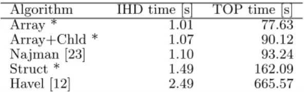
The edge extraction and sorting steps use the same code for all methods. Their computation time is included in the total time for all algorithms but it should not af-fect the difference. Table 1 summarizes the time required to construct the α-trees. All times were obtained by av-eraging times of 10 runs. The time for the IHD dataset is average for all 12 images.
The results provide several interesting observations. Complicating the construction algorithm so it creates smaller amount of redundant nodes pays off (the differ-ence between Najman and Array). The speedup seems
to depend on the size of the input graph. More signifi-cant difference is between the representation by structs and arrays. The results clearly show that the added flex-ibility of the representation does come with a significant additional cost.
The last algorithm is significantly slower. This de-serves deeper examination. The main difference is that the new algorithm uses the root finding structure com-pletely separated from the constructed tree. Our previ-ous work accesses the memory very sparsely and espe-cially for large graphs, almost every memory access leads to a cache miss. Moving the root-finding structure out-side of the tree seems to be a necessity.
Since the Structs and Arrays tree have significantly different capabilities, we included another test that con-structs a full child list for the arrays so the tree could be traversed similarly to the structs. It was done by count-ing the children, uscount-ing a prefix sum to calculate indices into the array of children and filling that array. It is in-teresting to notice that, even with these three additional passes, the tree construction is still faster than binary tree construction and postprocessing (this combination is called Array+Chld in Tab. 1).
4.3 Parallel tree construction
We finally evaluate the parallel tree (using structs data structure) construction on an SMT machine. 12 largest images of the IHD dataset were used to build an α-tree with l∞norm. The tests ran on an i72670QM processor
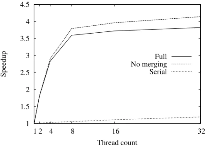
with 8GB ram. The CPU has 4 cores with hyperthread-ing. Figure 2 shows relative speedups for increasing num-ber of threads. 1 1.5 2 2.5 3 3.5 4 4.5 1 2 4 8 16 32 Speedup Thread count Full No merging Serial
Fig. 2 Tree construction speedup for increasing thread count. Graph shows speedup for building partial trees alone, full tree construction and serialized version.
Three graphs are given in Fig. 2, to measure speedups respectively for the full tree construction and the
con-Algorithm IHD time [s] TOP time [s] Array * 1.01 77.63 Array+Chld * 1.07 90.12 Najman [23] 1.10 93.24 Struct * 1.49 162.09 Havel [12] 2.49 665.57
Table 1 Performance of serial tree construction for IHD and TOP data. Contributions are marked with a star.
struction of partial trees only (without merging into the final tree). This roughly illustrates the maximal possible speedup that is limited by factors such as memory band-width. Third graph shows the speedup when the par-tial trees are constructed and merged in one thread. All graphs were generated by averaging measured speedups for individual images. Construction times were measured as an average of 10 attempts.
The parallel construction scales quite well with in-creasing number of threads. The flattening of speedup for more than 8 threads is not surprising due to number of virtual cores. However it is interesting that 8 threads perform significantly faster than 4. Since the virtual cores in hyperthreading share caches, for many parallel ap-plications hyperthreading brings almost no performance gain. Here hyperthreading brings measurable improve-ment. Since the algorithm accesses memory chaotically, the lower effective amount of cache available for each virtual core does not affect the performance too much.
Third graph shows that construction and merging of partial trees has small positive effect even when one thread is used. This is probably caused by less cache failures when only parts of the image are processed at once. 0.4 0.6 0.8 1 1.2 1.4 1.6 1.8 1 2 4 8 16 32 Speedup Thread count
Fig. 3 Tree construction speedup when node size is not com-pared during merging. Each line shows speedup for one IHD image. Wrong merging of nodes can completely negate the results in degenerate cases.
As mentioned in previous section, it is critical to merge nodes so children of a smaller one are moved to
larger one. Otherwise, for some degenerate images, the parallel construction can lead to a surprising slowdown. Figure 3 shows speedups for each image of the IHD dataset as a function of the thread count and illustrates this ef-fect. The slowdown is caused by the fact that merging nodes requires O(N ) reconnection of child nodes of the absorbed node. Which node of a merged pair has more children depends on the shape of the merged trees.
4.4 Effect of tree height on parallelization
Since the tree merging in parallel construction requires bottom-up tree traversal without any possible path com-pression, the tree height significantly affects the merging complexity. However since the number of edges processed during merging is relatively low, the resulting perfor-mance impact is not obvious.
To get a very high tree, we extended the IHD im-ages from 8b per channel up to 16b per channel with random low bits (similarly to [7]). In these synthetized data, the average tree height increased from roughly 80 for 8b images to 11000 for 16b images.
0 0.5 1 1.5 2 2.5 1 2 4 8 16 Time [s] Thread count 8b 10b 12b 14b 16b 1 1.5 2 2.5 3 3.5 4 1 2 4 8 16 Speedup Thread count 8b 10b 12b 14b 16b
Fig. 4 Left : Tree construction times for different bit depths. Right : The relative speedups for different bit depths.
Figure 4 (left) shows the average times as a function of the number of threads for various bit depths. Figure 4 (right) shows the relative speedup with increasing thread count for different bit depths. While the tree construc-tion slows down for increased image depth, parallel con-struction scales roughly the same for all image depths.
The tree depth does not affect the theoretical com-plexity of the singlethreaded construction, but it deffinitely affects the practical performance. Probably the main ef-fect is a higher number of tree nodes which results of higher memory consumption and more cache misses. The tree merging complexity depends on the tree height, but it does not affect the scaling in practice. The low number
of edges that connect partial trees is one cause. Also the merging does not always traverse the whole tree. Dur-ing lookup and zippDur-ing, the paths are not traversed in-dependently and if they converge, the merging immedi-ately ends. The gain from this optimization depents sig-nificantly on the tree structure, but we didn’t find any degenerate cases where it impacts the performance in a negative way.
5 Applications
Beyond experiments held to evaluate the performance of the algorithms proposed in this paper (see Sec. 4), we ad-dress here the impact of efficient tree construction meth-ods for modeling large visual data. To do so, we consider two different use cases, related to remotely-sensed im-age filtering and interactive video segmentation. These use cases are provided for illustration purpose only, thus explaining the lack of exhaustive comparison with the state-of-the-art.
5.1 VHR Remote Sensing
Earth observation through remote sensing technology benefits to a growing range of applications while facing new issues. Indeed, with the advent of very high reso-lution (VHR) sensors, satellite images are made of mil-lions or even bilmil-lions of pixels (called gigapixel images). The worldwide volume of such geospatial data is slowly reaching the Zettabyte scale. In this context, efficient means to access image content are required. Hierarchical structures like trees thus appear as a relevant model to represent such data.
Unsurprisingly, trees have been used in remote sens-ing to provide a multiscale description of image con-tent (see Sec. 2.2 and [29, 26, 18, 15, 45, 1]). Possible ap-plications include land cover/land use mapping (through supervised classification), crisis management with dam-age assessment (change detection/classification) or im-age understanding (e.g., with object detection). Trees have been built upon panchromatic (from optical or SAR sensors) as well as multi- or hyperspectral images.
To illustrate the relevance of hierarchical representa-tions in remote sensing, we consider the problem of image simplification, as already done by Brunner and Soille [6, 39] with α- and (α, ω)-connected components and trees. Image simplification aims at reducing the number of im-age elements to be processed, from elementary pixels to small regions or super pixels, and even to larger (and hopefully more meaningful) regions. As such, it of course eases image visualization, but it can also benefit to image compression or object-based image analysis (a paradigm that aims to consider regions as elementary units for im-age understanding in remote sensing). The interest of tree structures in this context relies in the fact that the
scale (impacting the number or size of regions) is easily tunable. Indeed, changing the scale parameter used in image simplification only requires a new scan and cut of the tree, while other techniques need to perform a full analysis on the pixels of the image.
We rely here on an α-tree where each node is also embedded with its global range (to be compared with the ω threshold). Image simplification is achieved through a cut of the tree, given an ω threshold (set relatively to the highest global range observed in the image, i.e. its global dynamics). Furthermore, a size criterion is applied to discard nodes smaller than a given threshold. This additional constraint is easily verified for each leaf of the tree cut at the ω level. It results in pixels or nodes filtered out of the image. A simple post processing can be employed here to assign these elements to their closest neighboring node (based on edge values).
We apply this strategy on the Vaihingen dataset that has been provided through the ISPRS benchmark on ur-ban object detection and 3D building reconstruction [10]. We consider here an aerial color images (16 bits) with a ground resolution below 10cm per pixel. The origi-nal data are provided together with a full mosaic of 20 250×21 300 pixels (called the TOP image in the previ-ous section). For the sake of clarity, we show here only a part (2 000 × 2 000 pixels) of the different images instead of the full original ones.
Simplification of the aerial color images is given in Fig. 5, where all images have been converted to 8-bit for visualization. We can visually observe the effect of the simplification process, that can also be measured quantitatively in terms of image elements: from 4 000 000 pixels in the original image, the simplification process returns 108 135 nodes (low area threshold, A > 1) or even only 2 583 nodes (high area threshold, A > 100). In other words, a compression ratio of more than 1:1 500 is achieved without no significant loss in terms of visible objects of interest. This allows subsequent steps to be much more scalable as well as relying on more meaning-ful information.
Finally, let us recall that, contrary to [6, 39], the com-putation time required by the simplification process is here not increasing with the scale but it is scale-independent. This is due to the method involved, i.e. a single cut of the tree instead of an iterative process, the tree having been computed offline very efficiently (e.g., see Tab. 1) with the algorithms presented in Sec. 3.
5.2 Interactive Object Selection in Video Sequences Another kind of visual data characterized by a large or very large volume is video sequences. Indeed, a video file is made of many frames or images acquired at a given framerate (most often 25 frames per second or fps). A simple 1 hour-long video sequence with VGA resolution (e.g., 640 × 480 pixels) and standard framerate (25 Hz) contains more than 27 billions of pixels.
(a) (b) (c) (d) Fig. 5 Simplification of an aerial color image (a) with ω threshold set to a tenth of the maximal observed global range, and various area thresholds: A > 1 (b) and A > 100 (c). Nodes filtered out are shown in black. Following a significant filtering A > 100, they are assigned to their closest neighbor (d). This removes small details and ”flattens” larger areas. Please zoom the pdf to see the details.
Such data require efficient management tools to be handled, e.g. through interactive multimedia editing tech-niques. A common process is to extract objects from videos, edit them and finally reintroduce the modified objects within the original video or another one. To al-lows this kind of video editing, interactive object selec-tion techniques are needed. Many approaches have been proposed in the last decade [5, 47, 4, 2, 33, 11, 25]. Never-theless, as shown by results achieved by the most re-cent techniques (e.g., [48] allows a processing framerate of 1.3-1.5 fps, far below current video broadcast stan-dards), there is still a lot of effort to be achieved in terms of computational efficiency. Even existing parallel strate-gies (e.g., [11]) do not allow for processing realistic videos (20 minutes are required to process a 40s video).
In this context, trees appear as a relevant solution and first results were promising [19]. We propose here to built upon our previous work [19] and we define the following strategy for interactive object selection.
First, a single tree is built from a video sequence, assuming space-time connectivity and representing the video as a spatio-temporal volume. Each pixel is then de-fined by a triplet (x, y, t) with two spatial and one tempo-ral coordinates. We define here the neighborhood using the 6-connectivity i.e., two pixels (x, y, t) and (x0, y0, t0) are neighbors if |x − x0| + |y − y0| + |t − t0| = 1. The
sim-ilarity measure is simply the Euclidean norm computed
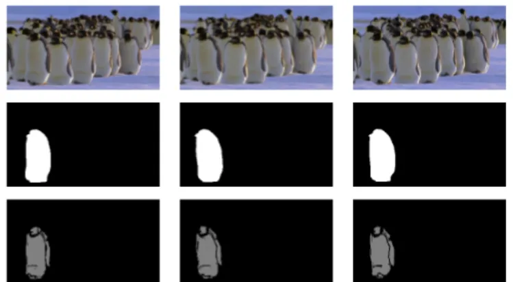
Fig. 6 Illustrative results of the tree-based object selection technique with the penguin video from SegTrack. From top to bottom: sample frames from the original sequence, associated ground truth, and extracted objects.
in the RGB color space. Of course other metrics could have been used, but let us recall that our goal here is not to provide the most accurate results, but rather to illus-trate the potential of tree representations for analyzing and processing large datasets. Furthermore, preliminary experiments achieved with the Lab color space did not lead to better results. Having defined the neighborhood and local similarity measure, the construction of the tree is straightforward using algorithms discussed in Sec. 3.
Following its computation, the tree becomes the im-age representation to be further processed (instead of the initial array of pixels). The interactive object selection scheme proposed here relies on the definition by the user of an object of interest. To do so, a user specifies a rect-angular selection through mouse clicking on any frame of the video sequence (for better accuracy, it is possible to set the selection in several frames simultaneously). We assume that the object of interest is completely included in the selection made by the user. This object (i.e., fore-ground) is then distinguished from the other parts of the video (i.e., background). To do so, we remove all back-ground nodes from the set of nodes included in the user selection, under the assumption that background nodes span outside the selection. Furthermore, noise robust-ness is ensured by filtering the small nodes, i.e. nodes with temporal duration below a given threshold.
To evaluate the relevance of such an approach, we consider a standard dataset and compare our results with the state-of-the-art. More precisely, we use the SegTrack dataset [44] that contains 6 video sequences, with length of 20–70 images of rather small size (from 320×240 pixels to 414 × 352 pixels), together with a reference segmen-tation (ground truth).
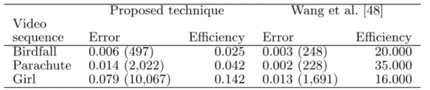
For the sake of illustration, we compare our method with one of the most recent works relying on this dataset [48] that requires a light input from the user, similarly to our method. Comparative results are provided in Tab. 2 using the same evaluation metrics than in [48]. Unsur-prisingly, the basic selection scheme described in this section (without any learning/modeling of the object,
nor any usage of motion/texture information) produces a higher error score than [48]. But on some challeng-ing videos like penguin, preliminary results are satis-factory as shown by Fig. 6, while many state-of-the-art techniques fail in this situation (with many similar ob-jects) [14, 32]. Indeed, more complex schemes for tree analysis still have to be explored and are out-of-the-scope of this paper.
A careful analysis of the weak results obtained by the proposed method with the Girl sequence leads to the fol-lowing observation. This video sequence is characterized by some important motion of the objects, whose visual impact consists in the lack of temporal connectivity be-tween the moving objects in the successive frames of the sequence. Besides, the video content is also blurred due to this motion effect. Furthermore, this video is charac-terized by a strong visual artefact consisting in an super-imposed watermark. With the α-tree model considered in this experiment, this leads to some spatio-temporal chaining effects that cannot be overcame without any post-processing or constrained imposed on the connec-tivity between pixels. Let us note that the artefacts due to high motion can be alleviated with high-speed videos. In this case, the proposed strategy looks very appealing due to its low complexity.
In spite of a loss in quality, the proposed tree model appears as an efficient image/video representation. As shown in Tab. 2, it offers a great improvement in terms of efficiency (ca. 3 orders of magnitude) over [48], which is one of the most efficient semi-supervised segmentation techniques (while unsupervised techniques are even more computationally expensive). It thus allows for introduc-tion of more complex (but still tree-based) image/video analysis strategies, to ensure both high quality and effi-ciency. To illustrate, let us recall that many video seg-mentation methods rely on a first segseg-mentation into su-perpixels, that might be easily produced by cutting the tree. But while extracting superpixels from a SegTrack video requires at least 500 seconds with the most effi-cient techniques from the state-of-the-art [51] (measured with a Dual Quad-core Intel Xeon CPU E5620 2.4 GHz, 16GB RAM running Linux), our algorithm is able to provide a set of superpixels in less than 50 seconds with a Java implementation and a standard laptop configu-ration (Dual-core Intel Core CPU i5-3320M 2.60GHz, 6GB RAM running Linux).
6 Conclusion
In this paper, we consider multiscale image representa-tion and analysis through tree models originated from Mathematical Morphology. Contrarily to component tree that have been extensively studied [8], but requires to set an ordering relation on the data (i.e. pixel values), we focus here on the α tree that relies on the edge values instead of pixel (vertex) ones. More precisely, two
re-cent α-tree construction algorithms were combined and incrementally inproved. This improved algorithm com-bines efficient single-threaded construction with the pos-sibility of parallelization and outperforms both. For the sake of research reproducibility and to support the use of the α-tree model and algorithms in various applications of image processing and computer vision, we have made the code available on Github1.
We also reviewed two possible data structures for tree representations, and compared them in terms of perfor-mance and flexibility. The representation by arrays of integers is significantly simpler and more efficient, but is not as flexible as dynamic structures linked by pointers. The difference is so significant, arrays should be used whenever possible, but the structures allow greater flex-ibility.
Finally, we have illustrated the possible interest of such tree models on several use cases, dealing with re-mote sensing image analysis and video segmentation. We have shown that the tree structure provides a very effi-cient way to process and analyse images of various na-tures.
While we show here how parallel construction of α-tree can be achieved with dynamic structures, design-ing such a solution with arrays is still very challengdesign-ing, contrarily to the case of min/max-tree. Indeed, efficient merging of such trees remains an open problem.
The merging of partial trees can be applied in many possible ways. The applications in this paper cover only a small subset. We plan to try this approach on other problems with large data (e.g., 3D volumes, long video sequences). In particular, such a strategy can be used for online processing of video streams to overcome the limitations related to memory requirements.
Acknowledgements
The authors would like to thank Michael Wilkinson for fruitful discussions and valuable suggestions, which helped in improving the manuscript.
The Vaihingen data set was provided by the Ger-man Society for Photogrammetry, Remote Sensing and Geoinformation (DGPF) [10].
References
1. A. Alonso-Gonzalez, S. Valero, J. Chanussot, C. Lopez-Martinez, and P. Salembier. Processing multidimensional sar and hyperspectral images with binary partition tree. Proceedings of the IEEE, 101(3):723–747, 2013.
2. X. Bai, J. Wang, D. Simons, and G. Sapiro. Video snap-cut: robust video object cutout using localized classifiers. In Proceedings of the SIGGRAPH, 2009.
1