HAL Id: hal-00699235
https://hal.inria.fr/hal-00699235
Submitted on 21 May 2012
HAL is a multi-disciplinary open access
archive for the deposit and dissemination of
sci-entific research documents, whether they are
pub-lished or not. The documents may come from
teaching and research institutions in France or
abroad, or from public or private research centers.
L’archive ouverte pluridisciplinaire HAL, est
destinée au dépôt et à la diffusion de documents
scientifiques de niveau recherche, publiés ou non,
émanant des établissements d’enseignement et de
recherche français ou étrangers, des laboratoires
publics ou privés.
Fault Localization in Constraint Programs
Nadjib Lazaar, Arnaud Gotlieb, Yahia Lebbah
To cite this version:
Nadjib Lazaar, Arnaud Gotlieb, Yahia Lebbah. Fault Localization in Constraint Programs. 22th Int.
Conf. on Tools with Artificial Intelligence (ICTAI’2010), 2010, Arras, France. �hal-00699235�
Fault localization in constraint programs
Nadjib Lazaar and Arnaud Gotlieb
INRIA Rennes Bretagne Atlantique, Campus Beaulieu, 35042
Rennes, France
Email: {nadjib.lazaar, arnaud.gotlieb}@inria.fr
Yahia Lebbah
Universit´e d’Oran, Lab. LITIO, 31000 Oran, Algeria Universit´e de Nice–Sophia Antipolis, I3S-CNRS, France
Email: ylebbah@gmail.com
—Constraint programs such as those written in high-level modeling languages (e.g., OPL [15], ZINC [14], or COMET [16]) must be thoroughly verified before being used in appli-cations. Detecting and localizing faults is therefore of great importance to lower the cost of the development of these constraint programs. In a previous work, we introduced a testing framework called CPTEST enabling automated test case generation for detecting non-conformities [13]. In this paper, we enhance this framework to introduce automatic fault localization in constraint programs. Our approach is based on constraint relaxation to identify the constraint that is responsible of a given fault. CPTEST is henceforth able to automatically localize faults in optimized OPL programs. We provide empirical evidence of the effectiveness of this approach on classical benchmark problems, namely Golomb rulers, n-queens, social golfer and car sequencing.
I. INTRODUCTION
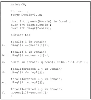
These last years have seen the explosion of high-level constraint modeling languages, including OPL [15], COMET [16], ZINC [14], or Essence [7]. In parallel, several propo-sitions were made to use constraint programs in critical applications. For example, constraint programs were developed for e-commerce [9], air-traffic control and management [6], [11] or critical software development [4], [8]. As any other programs, constraint programs written in high-level modeling languages must be thoroughly verified before being used on real-size instances of satisfaction or optimization problems. In [13], we introduced a testing framework where a first highly declarative constraint model is took as a reference to detect non-conformities within a refined and optimized constraint program solving the same problem. These non-conformities result from faults introduced during the refinement process, coming either from the absence or the bad formulation of constraints. Our testing framework was shown useful to detect non-conformities but it reveals itself poor at identifying the constraint responsible of the fault. In fact, the user resorts to explore manually one by one each of the constraints of its constraint model, which can be cumbersome even for small programs. For example, consider the N-queens problem solved by the OPL program of Fig.1. When N = 30, using a simple declarative model of N-queens, the testing framework of [13] reports a non-conformity: [30 29 28 ...1]. Although this vector indeed solves all the constraints of Fig.1, it shows a fault in the OPL program which obviously places many queens on the same diagonal. Therefore, at least one constraint of the model
using CP;
int n=...; range Domain=1..n;
dvar int queens[Domain] in Domain; dvar int diag1[Domain];
dvar int diag2[Domain];
subject to{
forall( i in Domain) a. diag1[i]==queens[i]+i;
forall( i in Domain) b. diag2[i]==queens[i]-i;
c. sum(i in Domain) queens[i]==(n*(n+1) div 2);
forall(ordered i,j in Domain) d. diag1[i]<=diag1[j];
forall(ordered i,j in Domain) e. diag2[i]!=diag2[j];
forall(ordered i,j in Domain) f. queens[i]!=queens[j];
}
Fig. 1:N-queens problem in OPL.
is incorrectly formulated. In this paper, we address the problem of automatically locating the constraint that is responsible of such a non-conformity. Automatic fault localization is a difficult problem, even for conventional programs. The most successful approach in the Software Engineering community is the Jones, Statsko and Harrold’s algorithm [10] that compares execution traces in order to guess the source code statements that are more likely to contain a fault. Their implementation called Tarantula takes both successful and unsuccessful execu-tion traces of a sequential program as inputs, and by crossing these traces, it ranks the statements from the most suspicious to the less suspicious. The idea of the ranking algorithm is that faulty statements more frequently appear on unsuccessful traces. A related approach proposed by Cleve and Zeller aims at tracing back the causes of fault introduction [3], which is the ultimate goal of fault localization. Recently, it has been shown that the Jones, Statsko and Harrold’s algorithm can be rephrased by using classical data mining indicators [1] leading to possible generalization to multi-faults localization. These approaches are well suited for sequential programs as the control flow is data-driven, i.e., any execution trace depends
on the values of input variables. However, they are not suited for constraint programs as the control flow is constraint-driven in this case, i.e., the order on which constraints are considered by the language interpreter is usually not determined by input values. In other words, comparing traces on distinct instances does not help to localize faults. A trend in constraint program debugging has been to analyze a single trace via generic trace models [5], [12]. In the context of the OADymPPaC1
project, several post-mortem trace analyzers such as Codeine for Prolog and Morphine [12] for Mercury, ILOG Gentra4CP, and JPalm/JChoco have been developed. All these tools can help the developer to understand and optimize his constraint program, but they are not dedicated to automatic fault localiza-tion. Following the Shapiro’s algorithmic debugging approach, the user still has to query the trace and user interaction during the debugging process is mandatory.
In this paper, we introduce a fault localization approach that is fully automated for OPL programs. This approach is based on systematic constraint relaxation by making use of the ILOG CP constraint solver. The idea is to solve auxiliary constraint programs built over the OPL constraint program under test and the reference model used to specify the problem. We provide an algorithm that takes the faulty constraint program and a non-conformity as inputs and returns either a single constraint or a set of constraints that are responsible of the fault. For example, in the OPL program of Fig.1, our algorithm reports constraint d as responsible of the given non-conformity. Look-ing at constraint d permits to spot that operator =< should be replaced by !=. We present our implementation called CPTEST enabling automatic fault localization. We provide empirical evidence on classical benchmark problems, namely golomb rulers, n-queens, social golfer and car sequencing that our approach is not only applicable but also efficient to localize faults in OPL programs.
The rest of the paper is organized as follows: Section II gives an overview of the constraint programs testing frame-work of [13] and introduces some notations. Section III presents our automatic fault localization algorithm. Section IV presents CPTEST and the empirical results we got on n-queens, golomb rulers, social golfers and car sequencing. Section V concludes this paper and draws some perspectives to this work.
II. BACKGROUND
CP aims at solving satisfaction or optimization problems. When one faces a problem specification, one usually writes down a first declarative constraint model that faithfully rep-resents the problem. We have high confidence in this model but playing with it rapidly shows that it cannot solve large instances of the problem. Then, this model is refined us-ing classical techniques such as constraint reformulation, re-dundant and surrogate constraint addition, global constraint replacement, or static symmetry-breaking constraints. This refinement leads to have an optimized constraint model tuned
1http://contraintes.inria.fr/OADymPPaC/
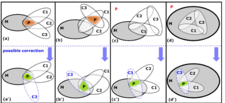
Fig. 2: Fault localization cases.
to address difficult instances. We think that most of the faults are introduced in this refinement step. In our previous work [13], we introduced a testing framework taking the first declarative model as an oracle for detecting non-conformities in the optimized model. We defined various formal conformity relations handling the cases where a single solution is found, all the solutions are found or a cost function has to be optimized.
A. Notations
In this section, we briefly give the necessary notations to understand the rest of the paper. M denotes the initial declarative model called the Model-Oracle and P denotes the Constraint Program Under Test (CPUT). Sol(M ) (resp. sol(P )) denotes the set of solutions of the model-oracle (resp. CPUT) where M possesses at least one solution(sol(M ) 6= ∅). Considering unsatisfiable model-oracles could be interesting for some applications but we excluded these cases in order to avoid considering equivalence of unsatisfiable models. The difference of two sets E and F is noted E\F , {x/(x ∈ E) ∧ (x /∈ F )}. The general conformity relation between the model-oracle M and the CPUT P is given by the following definition:
Definition 1 (conf ):
P conf M ⇔ sol(P ) 6= ∅ ∧ sol(P ) ⊆ sol(M )
B. Non-conformity detection
As proving conformity on any instance of a problem is undecidable in the general case, we have proposed in [13], test algorithms aiming at detecting non-conformities. For a given instance, a non-conformity is either a solution of the CPUT P that is not a solution of the model-oracle M , or P is reduced to fail (i.e., sol(P ) = ∅). Systematic non-conformities detection can be performed by combining the negation of a constraint of the model-oracle with the constraints of P (i.e., P ∧ ¬Ci
where Ci ∈ M ). Badly formulating a constraint in P can
remove and/or add solutions.
III. FAULT LOCALIZATION
Once a non-conformity is detected, one faces the problem of localizing the faulty constraint. The major requirement on which our approach is based is the single fault hypothesis,
i.e., there is only one constraint that is faulty in P . This requirement might appear as being restrictive but it has been shown that complex faults usually result from the coupling of single faults (a.k.a. the coupling effect [10]). In other words, faults that come from the interaction of several constraints are less likely to appear than single faulty constraint. Therefore, in our approach, when a non-conformity is found, we suppose that the CPUT P misses a single constraint or has only one faulty constraint in it.
A. Intuitions
Fig.2 depicts four distinct cases where the CPUT P does not conform the model oracle M (P ¬conf M ), i.e., there is a solution of P and not of M (part (a, b)) or sol(P ) = ∅ (part (c, d)), where P is a conjunction of three constraints C1∧ C2∧ C3. In Fig.2, P is represented by the intersection
of the three constraints and possible corrections are shown in blue.
• Part(a) exhibits a set of non-conformities (i.e., solutions
of P but not of M ) where P shares solutions with M (i.e., sol(M )∩sol(P ) 6= ∅). P is faulty as it contains C3a
badly formulated constraint such that sol(P )\sol(M ) 6= ∅. In fact, after having localized C3, this model could be
corrected as shown in part(a’).
• Part(b) exhibits another set of non-conformities where sol(P )\sol(M ) 6= ∅ and sol(M ) ∩ sol(P ) = ∅. In this example, we have
sol(M ) ∩ sol(C1) ∩ sol(C2) 6= ∅
sol(M ) ∩ sol(C1) ∩ sol(C3) = ∅
sol(M ) ∩ sol(C2) ∩ sol(C3) = ∅
hence, the faulty constraint can be localized as being C3.
Part(b’) shows a possible correction of P by revising C3.
• Part(c) exhibits a case where P is unsatisfiable. Here again, we have
sol(M ) ∩ sol(C1) ∩ sol(C2) 6= ∅
sol(M ) ∩ sol(C1) ∩ sol(C3) = ∅
sol(M ) ∩ sol(C2) ∩ sol(C3) = ∅
hence C3 is localized as the faulty constraint and should
be revised as proposed in part(c’).
• Finally, Part(d) shows a case where P is unsatisfiable
but differs from the previous one as
sol(M ) ∩ sol(C1) ∩ sol(C2) 6= ∅ ⇒ C3 may be faulty
sol(M ) ∩ sol(C1) ∩ sol(C3) 6= ∅ ⇒ C2 may be faulty
sol(M ) ∩ sol(C2) ∩ sol(C3) 6= ∅ ⇒ C1 may be faulty
In this case, the faulty constraint cannot be local-ized and the set {C1, C2, C3} is returned as an
over-approximation. In part(d’), we chose C3 as a possible
correction.
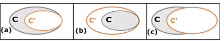
Fig. 3: Faulty constraint.
There are three distinct cases when considering non-conformities within P w.r.t. M : if C’ is a faulty version of a given constraint C, then C’ can either removes actual solutions (such as in part(a) in Fig.3), either add “new solutions” (part(b) in Fig.3) or both (part(c) in Fig.3).
B. The fault localization process
Our fault localization process is based on the following definitions and property. Formally speaking, given a CPUT P formed of {C1, C2, ...Cn} constraints that are not conform
w.r.t. its Model-Oracle M , then we introduce the notion of suspicious constraintas follows:
Definition 2 (Suspicious constraint): Ci is suspicious in P w.r.t. M
≡ M ∧ {C1, C2..., Ci−1, Ci+1...Cn} is satisfiable.
P does not conform M iff either P is unsatisfiable or there exists a non-conformity test case nc such as nc ∈ sol(P )\sol(M ). Our fault localization process aims at report-ing the set of suspicious constraints:
Definition 3 (SuspiciousSet): SuspiciousSet(P ) ≡ {C ∈ P : C is suspicious in P w.r.t. M }
In the example of Fig.2, the fault localization process will return Suspicious(P ) = {C1, C2, C3} for part(a) and part(d)
as no one of these three constraints may be faulty while it will return singleton {C3} for both part(b) and part(c),
showing that the faulty constraint is actually C3. Note that,
by construction, the set Suspicious(P ) is the smallest set containing all the suspicious constraints and then the over-approximation provided by this approach is also the more precise.
C. Algorithm
Based on the previous definitions, we propose an algorithm called locate that automatically localize suspicious constraints in P . Algo.1 takes as inputs the Model-Oracle M , the CPUT P and a non-conformity nc that has been automatically detected by other means [13]. The special case where P is unsatisfiable and then there is no nc is handled by a special tag. This algorithm returns SuspiciousSet(P ) noted rev({C1, .., Cm}) that may be a singleton in the most
favor-able case or all the constraints of P in the worst case. The algorithm returns also a second set addSet for the special case where all the constraints of P are suspicious, and a non-conformity point nc exists. In this case, nc satisfies P , but does not satisfy some single constraint in M , according to the testing process [13]. The checking algorithm computes addSet, the subset of M constraints that does not satisfy nc: some of these constraints could be caught in P in order to eliminate this non-conformity point.
Algorithm 1 locate(M, P, nc) 1: set ← ∅ 2: addSet ← ∅ 3: for each Ci∈ P do 4: if sol(M ∧ P \{Ci}) 6= ∅ then 5: set ← set ∪ {Ci} 6: end if 7: end for 8: if (set = P ) ∧ (nc 6= ∅) then 9: addSet ← checking(M, nc) 10: end if
11: return (rev(set), addSet) 12: 13: 14: checking(B, nc): 15: if B = ∅ then 16: return ∅ 17: else 18: for each Ci∈ B do 19: if nc |= Ci then 20: return checking(M \{Ci}, nc) 21: else 22: return {Ci}∪ checking(M \{Ci}, nc) 23: end if 24: end for 25: end if
D. Correctness and completeness
Providing that the underlying constraint solver is correct and complete, Algo.1 is correct as it will necessary return the faulty constraint within SuspiciousSet(P ). As sol(M ∧P \{Ci}) 6=
∅ is a sufficient condition for assessing that Ci is actually
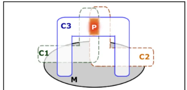
a faulty constraint and Algo.1 loops on all the constraints, no suspicious constraint can be missed. But, this condition is not necessary as, by hypothesis, only a single constraint is faulty. Thus, algo.1 is not complete and can return an over-approximation under the form of a set of suspicious constraints. Roughly speaking, algo.1 can return false alarms even in the case where a correct version of P is submitted for fault localization. Note also that Algo.1 can return all the constraints of P making the fault localization totally useless. Hopefully, this case is not frequent as it requires the conjunction of many unlikely events such as shown in Fig.4. In this example, there are three constraints where each pair of constraints shares common solutions.
IV. EXPERIMENTS
All our experiments were performed on Intel Core2 Duo CPU 2.40Ghz machine with 2.00 GB of RAM and all the models we used to perform these experiments are available online at (www.irisa.fr/celtique/lazaar/CPTEST).
A. CPTEST
In this section, we give a brief overview of CPTEST, a first testing framework for constraint programs written on
Fig. 4: Pathologic case
OPL. CPTEST includes a complete OPL parser and a backend process that produces dedicated OPL programs as output that have to be solved to detect and localize faults. The tool implements a process to detect fault and Algo.1 to localize this fault. CPTEST is based on ILOG CP optimizer 2.1.
The objective of our current experiment was to check that CPTEST can automatically detect and localize fault, using standard a fault injection process [2]. Then, we fed CPTEST with faulty CPUTs of four well-known CP problems, namely n-queens, social golfer, golomb rulers and car sequencing problems and we tried to localize faults by working on several instances from the easiest to the hardest.
B. n-queens problem
The problem of placing n queens on an n × n chessboard is a classical problem where the model-oracle can be given by three constraints (noted m_ct1,m_ct2 and m_ct3), the first one insures that all queens are placed differently on their column, the second and the third constraint insure that no two queens are placed on the same upper or lower-diagonal on the chessboard. We improved this model by adding new data structures, redundant, surrogate and global constraints. We have produced 7 different faulty CPUTs (P1 to P7)2 for
n-queens using fault injection.
Tab.I shows the results given by CPTEST on each faulty n-queens CPUT (n = 8). It shows the number of constraints and where fault was injected (e.g. p5_ct3 for P5), P6 and P7 are messing a part of n-queens specification where the fault injected respectively in p6_ct3 and p7_ct1 leads the CPUTs to accept new solutions. (part(b) Fig.3).
Tab.I shows also the non-conformity detected after the testing phase, the results of localization phase and its time con-sumption. P1, P2, P3 and P4 have no solution (sol(P i) = ∅) where the fault injected reduces them to fail. For instance let us take P3, the fault injected in is as follows:
p3_ct11: sum(i in Domain) queens[i]==(n*(n+1)/2);
turned to
p3_ct11: sum(i in Domain) queens[i]==(n+(n+1)/2);
2We recall that all models and CPUTs are available on
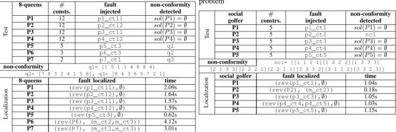
TABLE I: Fault detection and localization of n-queens problem
T
est
8-queens # fault non-conformity consts. injected detected P1 12 p1_ct11 sol(P 1) = ∅ P2 12 p2_ct12 sol(P 2) = ∅ P3 12 p3_ct11 sol(P 3) = ∅ P4 12 p4_ct12 sol(P 4) = ∅ P5 5 p5_ct3 q1 P6 3 p6_ct3 q2 P7 2 p7_ct1 q3 non-conformity q1= [1 5 1 1 4 8 8 4] q2= [7 8 3 2 4 1 5 6], q3= [8 4 3 6 5 7 2 1] Localization
8-queens fault localized time P1 (rev(p1_ct11),∅) 2.09s P2 (rev(p2_ct12),∅) 1.64s P3 (rev(p3_ct11),∅) 1.57s P4 (rev(p4_ct12),∅) 1.59s P5 (rev(p5_ct3),∅) 0.62s P6 (rev(P6), (m_ct2,m_ct3)) 4.12s P7 (rev(P7), (m_ct2,m_ct3)) 3.01s
CPTEST returns (rev(p3_ct11),∅) , here the set of suspicious constraint is the singleton p3_ct11 the faulty
constraint that has to be revised. The faults are localized for the four first programs in few seconds by pointing each time the faulty constraint that has to be revised.
The fault injected in P5 leads it to have bad n-queens solutions, testing phase highlights this non-conformity ([1 5 1 1 4 8 8 4]). For localization phase, CPTEST points the faulty constraint in less than a second and returns p5_ct3
to be revised.
For P6 and P7 the fault is that, respectively, p6_ct3 and p7_ct1do not catch a part of n-queens specification. The two CPUTs accept consequently new solutions. CPTEST detects non-conformities that are bad solutions revealing faults in P6 and P7. For localization, let us take P6, CPTEST returns
(rev(P6),(m_ct2,m_ct3)), in less than five seconds. The set
of suspicious constraint is here equals to P6, CPTEST returns also a set of M constraints (m_ct2, m_ct3) that should be considered in P6.
C. Social golfer problem
Social golfer is one of the famous problems in the CSPLib (prob010). We have m social golfers, n weeks and k groups of l size. Each golfer plays once a week in groups of l golfers. The problem is to build a schedule of play for all golfers over the n weeks such that no golfer plays in the same group as any other golfer more than one time.
The model-oracle can be built by two constraints ( m_ct1
and m_ct2 ), the first one to specify that each group has
exactly l golfers (group size). The second one to say that each pair of golfers meets only at most once.
The model-oracle can after be improved using static symmetry breaking. The symmetry can be broken by selective assignment. We get a model with five constraints, we inject
TABLE II: Fault detection and localization of social golfer problem
T
est
social # fault non-conformity golfer constrs. injected detected
P1 5 p1_ct1 sol(P 1) = ∅ P2 5 p2_ct2 nc1 P3 5 p3_ct3 sol(P 3) = ∅ P4 5 p4_ct4 sol(P 4) = ∅ P5 5 p5_ct5 sol(P 5) = ∅ non-conformity nc1= [[1 1 1 1][1 2 2 2][1 3 3 3] [2 1 3 3][2 2 2 1][2 2 1 1][3 3 3 2][3 1 1 2][3 3 2 3]] Localization
social golfer fault localized time P1 (rev(p1_ct1),∅) 1.04s P2 (rev(P2), (m_ct2)) 0.18s P3 (rev(p3_ct3),∅) 1.05s P4 (rev(p4_ct4,p4_ct5),∅) 1.03s P5 (rev(p5_ct5),∅) 1.15s
in each constraint a fault to get at the end five faulty CPUTs (P1 to P5). We launch CPTEST on these faulty CPUTs to first detect fault and after localize them. We take an instance of the problem with 9 golfers (3 groups of 3 golfers) playing during 4 weeks.
Tab.II shows the results given by CPTEST on each faulty CPUT. The fault injected in P1, P3 and P5 are respectively on
p1_ct1,p3_ct3andp5_ct5. These faults reduce the solution
space to empty for the three CPUTs, so there are non-conform to the model-oracle. For instance, let us take P5, the fault in
p5_ct5is:
p5_ct5: forall (g in 1..golfers, w in 1..weeks: w >= 2 && g <= groupSize ) assign[g,w] == g;
turned to
p5_ct5: forall (g in 1..golfers, w in 1..weeks: w >= 2 && g <= groupSize ) assign[g,g] == w;
CPTEST localizes the fault (in ' 1s) and returns the singleton p5_ct5 the constraint to be revised.
The fault injected in p2_ct2 leads P2 to accept new solutions. In this case, P2 can return bad solutions. CPTEST detects one of them by testing, nc1 is a non-conformity (a bad solution of social golfer) where golfer 3 and golfer 4 play in the same group (group3) over 2 weeks (3rd and 4th week). CPTEST returns (rev(P2),(m_ct2)) that the developer has to reformulate a constraint in P2 to catch (m_ct2) the second constraint of the model-oracle.
P4 is a case where CPTEST returns a set of suspicious con-straint. The fault is injected in p4_ct4 and CPTEST returns (p4_ct4, p4_ct5) an over-approximation of constraints. The two constraints in P4 break symmetries. Let us imagine that the search space SR can be divided in two symmetric sets: SR ≡ S1∪ S2where p4_ct5 removes S2. p4_ct4 divides
S1 in two symmetric sets (S1 ≡ S3∪ S4) and removes S4.
By adding the two constraints, the search space is reduced to S3. The fault injected to p4_ct4 removes S1where p4_ct5
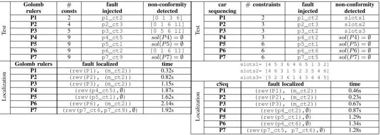
TABLE III: Fault detection and localization of Golomb rulers problem
T
est
Golomb # fault non-conformity rulers consts injected detected
P1 2 p1_ct2 [0 1 3 6] P2 4 p2_ct3 [0 1 6 11] P3 5 p3_ct3 [0 5 6 11] P4 9 p4_ct5 sol(P 4) = ∅ P5 9 p5_ct1 sol(P 5) = ∅ P6 9 p6_ct2 [0 1 6 11] P7 9 p7_ct9 sol(P 7) = ∅ Localization
Golomb rulers fault localized time P1 (rev(P1), (m_ct2)) 0.32s P2 (rev(P2), (m_ct2)) 0.82s P3 (rev(P3), (m_ct2)) 1.15s P4 (rev(p4_ct5),∅) 1.87s P5 (rev(p5_ct1),∅) 1.62s P6 (rev(P6), (m_ct2)) 2.14s P7 (rev(p7_ct6,p7_ct9),∅) 1.92s
removes S2, in this case the search space is reduced to empty
and either p4_ct4 or p4_ct5 can be revised.
D. Golomb rulers
A Golomb ruler is a set of m marks ( 0 = x1< x2... < xm)
where the m(m − 1)/2 distances {xj− xi|1 ≤ i < j ≤ m}
are distinct. A ruler is of order m and its length is xm. The
objective is to find an optimal ruler (minimal length) of order m.
A first declarative model (model-oracle) includes two constraints. m_ct1 to order the marks and m_ct2 to have different distances between these marks.
We improve this model using different techniques, the use of new data structure (e.g. d for distances), the addition of a global constraint (allDifferent(d)), the addition of surrogate and redundant constraints. We also break symmetry by adding specific constraints. We obtain at the end 7 faulty CPUT by fault injection.
We take a small instance of Golomb rulers (m = 4). We launch CPTEST on these faulty CPUTs where Tab.III shows the results. The three first CPUTs accept new solutions where the fault injected is of type part(b) Fig.3. For each of these three CPUTs a non-conformity is reached. For example, if we take P2, CPTEST returns after testing [0 1 6 11] that is a bad Golomb ruler where 6-1=11-6. CPTEST returns after localization (rev(P2),(m_ct2)), here P2 has to catch the second constraint of the model-oracle by reformulating one of its constraints.
P4 and P5 are also non-conform to the model-oracle where sol(P i) = ∅. The faults are respectively in p4_ct5 and p5_ct1. Let us take P4 to show the injected fault:
p4_ct5: allDifferent(all(ind in indexes ) d[ind]);
turned to
p4_ct5: forall(i in m..2*m)
count(all(j in indexes) d[j],i)==1;
TABLE IV: Fault detection and localization of car sequencing problem
T
est
car # constraints fault non-conformity sequencing injected detected
P1 2 p1_ct2 slots1 P2 3 p2_ct3 slots2 P3 3 p3_ct2 slots3 P4 3 p4_ct2 sol(P 4) = ∅ P5 6 p5_ct1 sol(P 5) = ∅ P6 6 p6_ct6 sol(P 6) = ∅ P7 6 p7_ct5 sol(P 7) = ∅ slots1= [4 5 3 6 4 6 5 1 3 2] slots2= [4 6 3 1 5 2 3 5 4 6] slots3= [5 2 3 6 1 4 3 6 4 5] Localization
cSeq fault localized time P1 (rev(P1), (m_ct2)) 0.46s P2 (rev(P2), (m_ct2)) 0.23s P3 (rev(P3), (m_ct2)) 0.67s P4 (rev(p4_ct2),∅) 0.87s P5 (rev(p5_ct1),∅) 1.29s P6 (rev(p6_ct6),∅) 1.34s P7 (rev(p7_ct5, p7_ct6),∅) 1.28s
CPTEST returns a singleton as suspecious constraints set for P4 and P5 (resp. p4_ct5 and p5_ct1) in a reasonable time consumption.
P6 have a bad formulation on p6_ct2 and CPTEST returns a non-conformity. For localization, CPTEST returns m_ct2 to be caught in P6.
On P7, we injected one fault at p7_ct9 (6= turned to =). This fault reduces sol(P 7) to empty. CPTEST returns two suspicious constraints (p7_ct6 and p7_ct9). This is due to the interference created by the injected fault between the faulty p7_ct9 and p7_ct6 where the two constraints are dedicated to a static symmetry breaking.
E. Car sequencing
Car sequencing is an interesting CP problem that tries to find an assembly line of cars for a car-production company where cars are grouped on classes. Each class represents cars with some specific options. The assembly line must satisfy some option capacity constraints.
The model-oracle of car sequencing is taken from the OPL book [15]. The model-oracle is composed of two constraints (m_ct1 and m_ct2). The first one expresses demand constraints for how many cars of a given class have to be produced. The second one expresses capacity constraints of the form l outof u for: Each sub-sequence of u cars, a unit can produce at most l cars with a given option.
We improve the original model and we follow the same approach as for the precedent problems by injecting faults. We have at the end 7 faulty CPUTs.
We took an instance of the problem with an assembly line of 10 cars, 6 classes and 5 options. Tab.IV shows the results of CPTEST for fault detection and localization on car sequencing problem.
The three first CPUTs (P1, P2 and P3) have the same characteristics that accept new solutions and are non-conform
to the model-oracle, the faults are injected respectively in p1_ct2, p2_ct3 and p3_ct2. CPTEST returns a non-conformity point for the three first CPUTs (resp. slots1, slots2 and slots3) that are bad assembly lines. To localize faults, CPTEST returns all constraints as an over-approximation. It proposes a model-oracle constraint m_ct2 to be caught in the CPUTs.
P4, P5 and P6 have a faulty constraint (resp. p4_ct2, p5_ct1 and p6_ct6). The faults injected in these CPUTs reduce the set of solutions to empty and CPTEST detects this non-conformity.
If we take P5, the fault injected is a bad formulation as:
p5_ct1: forall(i in Cars) sum(j in Slots) ((slot[j]==i)*(one[j]))==demandV[i];
turned to
p5_ct1: pack(slot, slot, one);
This constraint is returned by CPTEST ((rev(ct1),∅) in 1.29s.
In P7, the fault is injected in p7_ct5 where P7 is non-conform to the model-oracle. CPTEST returns in localization a set of suspicious constraints (p7_ct5, p7_ct6).
V. CONCLUSION
In this paper, we introduced a novel approach for automatic fault localization in constraint programs. According to our knowledge, this is the first time an approach that is not based on post-mortem trace analysis is proposed: the advantage being that our approach does not require any user interaction. We enhanced CPTEST, our CP testing framework for OPL pro-grams, with automatic fault localization. And we got empirical evidence that shows our approach is efficient to localize fault in OPL programs. The experimental evaluation was performed on classical benchmarks such as Golomb rulers, n-queens, social golfers and car sequencing. In many cases, CPTEST can localize exactly the constraint responsible of a reported non-conformity efficiently. In a few cases, several constraints are proposed among which the faulty constraint is necessarily included. However, our approach is currently built on the hypothesis that a single constraint is responsible of the non-conformity which is a limitation. Further work includes the removal of this limitation as well as the extension of CPTEST to automatic correction of faulty constraints.
REFERENCES
[1] Peggy Cellier, Mireille Ducass´e, S´ebastien Ferr´e, and Olivier Ridoux. Dellis: A data mining process for fault localization. In Proc. of the 21st International Conference on Software Engineering & Knowledge Engineering (SEKE’2009), pages 432–437, 2009.
[2] Jeffrey A. Clark and Dhiraj K. Pradhan. Fault injection. Computer, 28(6):47–56, 1995.
[3] Holger Cleve and Andreas Zeller. Locating causes of program failures. In ICSE ’05: Proceedings of the 27th international conference on Software engineering, pages 342–351, New York, NY, USA, May 2005. [4] H. Collavizza, M. Rueher, and P. Van Hentenryck. Cpbpv: A constraint-programming framework for bounded program verification. In Proc. of CP2008, LNCS 5202, pages 327–341, 2008.
[5] P. Deransart, M. V. Hermenegildo, and J. Maluszynski, editors. Analysis and Visualization Tools for Constraint Programming, Constrain Debug-ging (DiSCiPl project), volume 1870 of Lecture Notes in Computer Science. Springer, 2000.
[6] P. Flener, J. Pearson, M. Agren, Garcia-Avello C., M. Celiktin, and S. Dissing. Air-traffic complexity resolution in multi-sector planning. Journal of Air Transport Management, 13(6):323 – 328, 2007. [7] A.M. Frisch, M. Grum, C. Jefferson, B. Martnez, and H.I. Miguel. The
design of essence: a constraint language for specifying combinatorial problems. In Proceedings of IJCAI’07, pages 80–87, 2007.
[8] A. Gotlieb. Tcas software verification using constraint programming. The Knowledge Engineering Review, 2009. Accepted for publication. [9] Alan Holland and Barry O’Sullivan. Robust solutions for combinatorial
auctions. In ACM Conference on Electronic Commerce (EC-2005), pages 183–192, 2005.
[10] J. A. Jones, M. J. Harrold, and J. Stasko. Visualization of test information to assist fault localization. In ICSE ’02: Proceedings of the 24th International Conference on Software Engineering, pages 467– 477, 2002.
[11] U. Junker and D. Vidal. Air traffic flow management with ilog cp optimizer. In International Workshop on Constraint Programming for Air Traffic Control and Management, 2008. 7th EuroControl Innovative Research Workshop and Exhibition (INO’08).
[12] L. Langevine, P. Deransart, M. Ducass´e, and E. Jahier. Prototyping clp(fd) tracers: a trace model and an experimental validation environ-ment. In WLPE, 2001.
[13] N. Lazaar, A. Gotlieb, and Y. Lebbah. On testing constraint programs. In Proc. of Principles of Constraint Programming, CP’2010, Sept. 2010. [14] K. Marriott, N. Nethercote, R. Rafeh, P. J. Stuckey, M. Garcia De La Banda, and M. Wallace. The design of the zinc modelling language. Constraints, 13(3):229–267, 2008.
[15] P. Van Hentenryck. The OPL optimization programming language. MIT Press, Cambridge, MA, USA, 1999.
[16] Pascal Van Hentenryck and Laurent Michel. Constraint-Based Local Search. The MIT Press, 2005.