l1-norm Minimization Based Algorithm for Non-Intrusive Load Monitoring

(1)

HAL Id: hal-01253514

https://hal.inria.fr/hal-01253514

Submitted on 12 Jan 2016

HAL is a multi-disciplinary open access

archive for the deposit and dissemination of

sci-entific research documents, whether they are

pub-lished or not. The documents may come from

teaching and research institutions in France or

abroad, or from public or private research centers.

L’archive ouverte pluridisciplinaire HAL, est

destinée au dépôt et à la diffusion de documents

scientifiques de niveau recherche, publiés ou non,

émanant des établissements d’enseignement et de

recherche français ou étrangers, des laboratoires

publics ou privés.

Xuan-Chien Le, Baptiste Vrigneau, Olivier Sentieys

To cite this version:

Xuan-Chien Le, Baptiste Vrigneau, Olivier Sentieys. l1-norm Minimization Based Algorithm for

Non-Intrusive Load Monitoring. IEEE International Conference on Pervasive Computing and

Com-munication Workshops (PerCom Workshops), IEEE Workshop on Pervasive Energy Services, Mar

2015, St. Louis, United States. pp.299 - 304, �10.1109/PERCOMW.2015.7134052�. �hal-01253514�

(2)

l1

-norm Minimization Based Algorithm for

Non-Intrusive Load Monitoring

Xuan-Chien LE, Baptiste VRIGNEAU, Olivier SENTIEYS

IRISA/INRIA, University of Rennes 1 6 Rue Kerampont, 22300 Lannion, France {xuan-chien.le, baptiste.vrigneau, olivier.sentieys}@irisa.fr

Abstract—Non-Intrusive Load Monitoring (NILM) plays an important role in energy management and energy reduction in buildings and homes. An NILM system does not need a large amount of deployed power meters to monitor the power usage of home devices. Instead, only one meter on the main power line is necessary to detect and identify the operating devices. There are many approaches to solve the problem of device determination in NILM. The features applied in low-frequency based approach essentially include the step-change (or edge) and the steady state. This paper introduces three algorithms to solve the l1-norm minimization problem in NILM and results on power measurements obtained from a real appliance deployment. With a small number of devices, the obtained precision varies from 75% to 99%, depending on the tolerance criterion to determine the steady state of a given device.

I. INTRODUCTION

Appliance load monitoring systems nowadays play an im-portant role in energy management in buildings and homes, especially in Smart Building Automation, where the electronic appliances can be fluctuated to adapt to the variation of environment based on the gathered information. There are many methods to implement the system and they can be classified into two approaches: intrusive and non-intrusive. In the intrusive approach, the measurement is deployed at each individual equipment, each meter gets the data from the device it monitors. Retrieved data can be the power consumption if power meters are used, that is also considered as direct sensing, or information about the environment captured by the sensors such as light intensity, vibration, sound, etc., which are generated by the monitored device and imply the operation state of them, that is so-called indirect sensing. A supervision system combining these two methods of sensing is introduced in [1] and known as ViridiScope. In this system, the devices which consume a stable power are individually monitored by one or some specific sensors such as light sensors, acoustic sensors, while the variable loads are supervised by magnetic sensors or direct power meters. In spite of high accuracy, high deployment cost prevents the intrusive approach from widely being applied. Instead, the non-intrusive approach, which can detect and estimate the power consumption of all devices in the monitored area with only one power meter deployed on the main power line, is more attractive. In the remaining of this paper, the related works of Non-Intrusive Load Monitoring (NILM) will be mentioned in Section 2. Then the sensor deployment to gather the data inside our

laboratory is presented in Section 3. Section 4 introduces our proposed approach using l1-norm minimization and the simulation to solve the problem in the context of NILM, while Section 5 shows the results as well as the evaluation metrics to evaluate the algorithm. Finally, some conclusions are given in Section 6

II. RELATED WORKS

In [2], the original problem of NILM is introduced. They use an edge detector to detect the events on the aggregate power draw, which corresponds to the operation periods of devices, cluster and match them with the pre-defined features in library. Because there are some fluctuations when a device is switched on/off or during the steady state due to noise, the power data can pass through a median filter [3] or a pre-processing block [4] before detecting and identifying the events. In these researches, the length of each event is not considered, only the step-changes are used as identified features. Hence, the authors of [5] propose to apply Dynamic Time Warping (DTW), a time-series-based approach to compare two vectors with different lengths and non-identical values, to match the events. Every time an event is detected, the distances between it and all features in library are calculated. The event will be identified to the device whose feature leads to the minimum distance. The precision of this method varies from 85% to 99% depending on the type of house.

In addition, other researches apply the advance models such as Hidden Markov Model (HMM) combining with Viterbi dis-aggregation [6], [7] and Artificial Neural Network (ANN) [8]. While the authors of [6] use the difference on aggregate power usage between the current instant and previous instant as the observation of HMM, Kim and his colleagues in [7] use the current aggregate power but combine with the additional fea-tures such as time of day, day of week or information from the environment monitoring sensors to create a variant of HMM so-called Conditional Factorial Hidden Semi-Markov Model (CFHSMM). While the HMM-based NILM is tested with different types of household, the ANN in [8] is only applied to identify and estimate the power usage of two groups: H (water heater) and W (washing machine, dish washer). The data of one day sampled every 15 minutes and devided into six 8-hour segments is the input of an ANN, whose output includes two possibilities: H and W . Nevertheless, with the accuracy from 72% to 99% for HMM-based method and over

(3)

90% for ANN-based one, both of them have a perspective to extend their application to larger amount of devices.

However, DTW, HMM and ANN methods need a long training period to analyze the characteristics and learn the parameters of the devices. Therefore, this paper introduces a new approach using the l1-norm minimization and requiring a short training. Because the l1-norm minimization problem relates to the Least Absolute Error (LAE) value, in the remaining of this paper, this approach is called LAE-based method. Moreover, two optimized versions of this approach are also presented including difference-based method, which considers the previous state of devices in determining their current state, and probability-based method that uses the state transition probability as a criterion for state determination. The simulation results of these three methods will then be compared with the edge detection-based approach mentioned in [2]. The dataset using for the simulation is collected by the smart power meters. They collect the power consumption of monitored devices at 1 Hz frequency and support the Zigbee wireless communication. The data from this measuring system will be used to create the test power draw for NILM algorithm and as ground truth data to evaluate the accuracy. The l1-norm minimization problem in NILM is then simulated in Matlab for a small set of devices such as fridge, television, microwave, teapot, coffee machine. These devices are in the the coffee room and usually used during the coffee break. Because they consume at one or two stable power levels, one day is enough to find the average power demand of each steady state. Besides solving the minimization problem, the past state of each device is also taken into account to find the current state to increase the accuracy.

III. SENSOR DEPLOYMENT

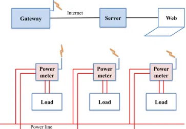
In order to observe and analyze the power consumption characteristic of electric devices, a smart power meter grid is deployed on the third floor of our laboratory. In this system, the wireless network is supplied by the Athemium

Server Power line Power meter Load Power meter Load Power meter Load

Gateway Internet Web

Fig. 1: Smart meter grid to observe and analyze the power consumption characteristic of electric devices.

TABLE I: Average power consumption of the steady states of some devices in the coffee room.

Average power 1 (watt) Average power 2 (watt) Fridge [75.89, 75.96]

Television [200.54, 202.11] 29.00 Microwave [1332.04, 1356.18] [1282.50, 1317.95]

Teapot [1665.29, 1675.81] Coffee machine [823.05, 830.06]

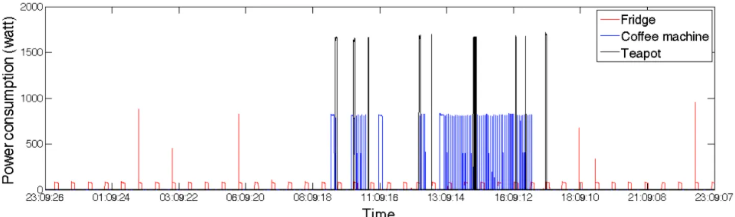
company [9], which supports Zigbee wireless communication and sends the gathered data to the Athemium server through the gateways, while each device is monitored by an individual power meter Z-800 of Netvox Technology Company [10]. The users can observe the data and download it to their personal drive through a web interface. The monitored devices include laptops, desktops, screens, external drivers, printers in the offices and electrical equipment in the coffee room such as fridge, television, microwave, teapot and coffee machine. Their power usage is sampled and periodically reported to the server every one second. The system model is illustrated in Figure 1 and an example of retrieved data over time of several popular appliances such as fridge, teapot, coffee machine is shown in Figure 2. These devices have one levels of power demand: the fridge has a spike at the transient phase and then consumes a stable power of 76 watts; the coffee machine consumes about 825 watts; while the teapot uses over 1600 watts of power when operating. This characteristic allows to use the steady state as a feature to identify the devices. The identification methods can be based on the edge detector as in [2] or the distance between the detected steady events and the pre-defined features from the training period [5]. However, in this paper, we solve the l1-norm minimization mentioned in [2] in order to determine the operation states of all devices. The dataset for the simulation is retrieved by the power meters during two weeks and includes the power consumption of five devices in the coffee room: fridge, television, microwave, teapot and coffee machine. This dataset is considered as the ground truth data for algorithm evaluation and to synthesize the aggregate power usage by adding the power consumption of all devices with a small noise created from the power meters. The concrete average power consumption of the steady states of five devices used in the simulation are shown in Table I. A steady state is only listed in this table if its appearance probability is larger than 1%, that is the reason why there are some times the coffee machine consumes about 400 watts but that value is ignored. Three of five devices have only one level of power consumption including fridge, teapot and coffee machine, as presented in Figure 2, while two others have two power states. The difference on the power level between the devices is large, so the small noise will not affect the performance of the algorithm. Therefore, for simplicity, we choose the normal distribution noise with zero mean and variance of 1 watt when synthesizing the aggregate power consumption.

(4)

Fig. 2: Retrieved power consumption of three devices: fridge, coffee machine and teapot on Sept. 8th, 2014. Average power Tolerance Steady P O W E R TIME

Fig. 3: Steady state passing the transient [2].

IV. STATE DETERMINATION ALGORITHM

Different from the minimization problem in [2], which assumes that each device has only two states ON and OFF, in this paper, each device i ∈ {1, . . . , N } can operate in one of Mi states. Denote sij(t) as the Boolean indicator of being in

the j − th state of i − th device at time t, j ∈ {1, . . . , Mi}:

sij(t) =

(

1 if device i operates in state j

0 if device i does not operate in state j,

the aggregate power consumption can be represented as fol-lows: x(t) = N X i=1 Mi X j=1 sij(t) × wij+ e(t), (1)

where x(t) is the aggregate power at time t, wij is the average

power of the i − th device when it operates in state j and e(t) is a noise. To determine the value of wij, a transient-passing

steady state detector finds on the power time-series the periods in which the power does not vary larger than the tolerance value, as illustrated in Figure 3. wij is therefore calculated by

averaging the data points in the corresponding steady period.

A. LAE-based method

From the model of Equation (1), the indicator vector s can be determined by solving the following l1-norm minimization:

min s k x(t) − N X i=1 Mi X j=1 sij(t) × wij k subject to: ( sij(t) ∈ {0, 1}, ∀{i, j} PMi j=1sij(t) ∈ {0, 1}, ∀i. (2)

The respective solution is:

ˆ s(t) = arg min s k x(t) − N X i=1 Mi X j=1 sij(t) × wij k. (3)

To solve (2), the condition is at first processed by finding all possible combinations of state vector s and writing them in matrix S, of which each row relates to a combination. For example, if we have two devices and each of them has two operation states, all possible combinations are saved in matrix S as follows: S =               0 0 0 0 0 0 0 1 0 1 0 1 0 1 0 0 0 1 1 0 0 0 1 0 1 0 1 0 1 0 0 0 1 0 0 1              

After that, all combinations will be in turn applied to expres-sion (4) to calculate the absolute error corresponding to each case:

AE(k) = |x(t) − s(k)× wT|, (4) where s(k) _{is the k − th row of S. The combination giving}

(5)

B. Difference-based method

However, the LAE value may not be the solution of the NILM problem. In real condition, the power consumption of each device can have some variations, the real state of devices does not lead to minimum absolute error but a value around it. For more accuracy, a supplemented constraint is proposed: among possible combinations which lead to near-minimum error, the solution is the one, which has least change in comparison with the previous state. If existing any combination which has the absolute error near to the LAE value, it will be saved as a candidate, along with ˆs, for the final consideration. In the final step, the candidate, which has least change in comparing with the previous state, is chosen as the current state of the system, or:

˜

s = arg min

sc∈SC

|sc⊕ s(t − 1)|, (5)

with SC the set of candidates. Algorithm 1 clarifies this

method. The value of threshold in our simulation is empir-Algorithm 1 l1-norm minimization algorithm based on the difference with the previous state.

1: function L1SOLVE(x, w)

2: Find possible combinations of s and save in matrix S

ically chosen to be of 2 watts. If this value is too small, the real solution of s may be rejected from the set of candidates, while large value increases the number of candidates and the possibility of error detection.

C. Probability-based method

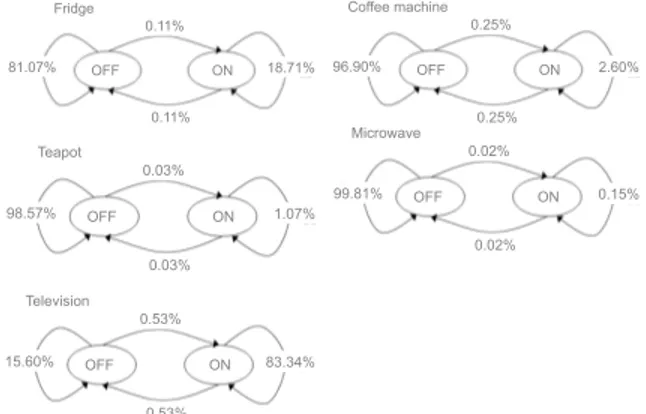
Instead of determining the difference between the candidates and the previous state, we can also consider the state transition probability p(si(t)|si(t − 1)) of each device to decide the

current state, as detailed in Algorithm 2. This conditional probability is obtained by analyzing the training data. The state transition probability some devices is presented in Figure 4. The probability for current state determination is the product of state transition probability of all devices, or:

P r(s(t)|s(t − 1)) =

N

Y

i=1

p((si(t)|si(t − 1)), (6)

where p((si(t)|si(t − 1)) is the state transition probability of

device i. In this method, we do not separately consider each steady state of device but only consider if that device is on or off. The state that makes the largest probability in (6) will be decided as the current state of the system.

OFF ON 0.25% 0.25% 96.90% 2.60% OFF ON 0.11% 0.11% 81.07% 18.71% OFF ON 0.02% 0.02% 99.81% 0.15% Microwave OFF ON 0.53% 0.53% 15.60% 83.34% Television OFF ON 0.03% 0.03% 98.57% 1.07% Teapot

Fig. 4: State transition probability of fridge, coffee machine, teapot, microwave and television during the training period.

Algorithm 2 l1-norm minimization algorithm based on the state transition probability.

1: function L1SOLVE(x, w)

2: Find possible combinations of s and save in matrix S

In this section, we test the proposed methods with five devices in the coffee room: fridge, coffee machine, teapot, microwave and television. The data received from the power meters deployed for each individual devices are used as the ground truth data for evaluation and to create the aggregate power by combining them with a normal distribution noise with zero mean and variance of 1 watt. The training and testing data was gathered from two weeks in September 2014. The algorithm to solve the l1-norm minimization is then simulated in Matlab to find the states of those devices. To evaluate this algorithm, we use two metrics: precision and recall. Precision is defined as the ratio between the number of good detections and the total number of detections, while recall is defined as the ratio between the number of good detections and the total number of events including the detected events and undetected events. They are calculated as follows:

precision = T P

T P + F P (7) recall = T P

T P + F N, (8) where TP, FP, FN are true positive, false positive and false negative, respectively, and defined as:

(6)

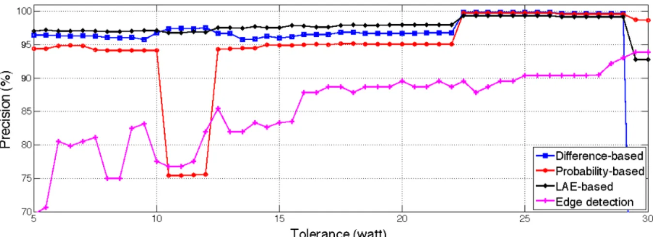
Fig. 5: Precision of l1-norm minimization algorithm vs. power tolerance for steady state determination.

• If an appliance is ON and it is detected as ON by the algorithm, a true positive is taken into account.

• If an appliance is OFF but it is detected as ON by the algorithm, a false positive is taken into account.

• If an appliance is ON but its state is not detected, then the result is a false negative.

Figure 5 represents the precision of the three proposed methods of l1-norm minimization based algorithm in compar-ison with the edge detection-based algorithm introduced in [2] when tuning the tolerance value from 5 watts to 30 watts. The first method (LAE-based) does not consider the previous state of each device, while the second one (difference-based) uses the difference between the current state and previous state, and the third one (probability-based) applies the state transition probability. The purpose of this experiment is to test the possibility of applying the l1-norm minimization to solve the problem in the context of NILM, so only the edge detection-based algorithm is used for result comparison. Other methods such as ANN, HMM are more complex and need a long training period to analyse and synthesize the characteristics of the devices, so they will not be compared in this paper. The simulation results in Figure 5 show that the precision in the three cases outperforms the edge-based approach. With the tolerance value larger than 22.5 watts, the precision is improved when considering the previous state. However, with the second method, the precision falls down to under 30% when the tolerance exceeds 29 watts. This result can be explained as follows: when the tolerance value is small, the number of stable periods will intuitively increase. However, some of them do not last at least the minimum length to be able to be considered as a steady state. They will be suppressed from the library and lead to the wrong detection. Besides, if the tolerance value is over 29 watts, the precision of the second method quickly decreases to lower than 30%. This result comes from the fact that the television consumes 29 watts in stand-by mode. During the testing period, it almost operated in this mode. Additionally, the method is based on the difference with the previous state, while the start state of

TABLE II: Maximum, minimum, average and standard devi-ation of precision.

Max (%) Min (%) Avg (%) Stdev (%) Edge-based 93.04 69.63 85.03 5.78 LAE-based 99.36 96.75 97.98 0.91 Difference-based 99.88 95.74 97.48 1.53 Probability-based 99.77 75.38 94.58 6.18

TABLE III: Maximum, minimum, average and standard devi-ation of recall.

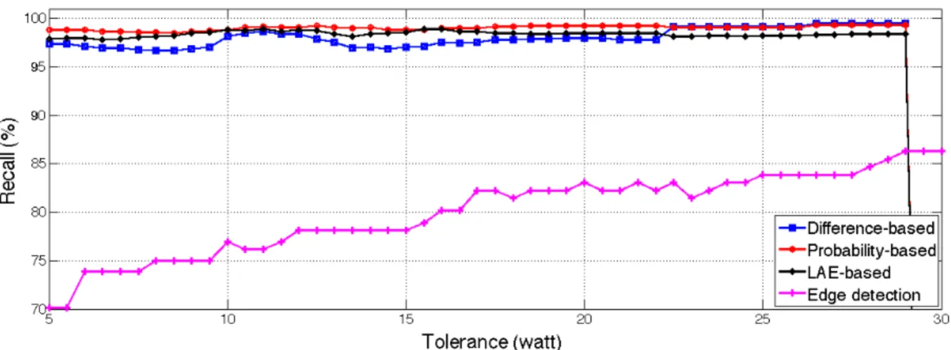
Max (%) Min (%) Avg (%) Stdev (%) Edge-based 86.29 70.15 79.72 4.06 LAE-based 98.91 97.83 98.39 0.28 Difference-based 99.50 96.68 98.04 0.94 Probability-based 99.34 98.47 99.04 0.23

the television is always off, so the system could not detect exactly. Meanwhile, with the third method, which is based on the state transition probability, the probability to maintain the stand-by mode is much larger than that to maintain the off state. Hence, the precision does not decrease too much. Figure 6 represents the recall metric of the four approaches versus the value of tolerance. This figure shows that the recall falls down less than 20% when the tolerance is larger than 29 watts in the three methods based on the l1-norm minimization based algorithm. Because the recall relates to the undetected events, the result means that there are many time instants where the devices operate but the algorithm cannot detect. The maximum, minimum, average and standard deviation values of the precision and recall are given in Table II and Table III, which imply that the LAE-based algorithm is less dependent on the value of tolerance, while the edge detection-based strongly depends on this parameter.

VI. CONCLUSION

NILM is a very important in energy management and saving. There are many researches focusing on processing

(7)

Fig. 6: Recall l1-norm minimization algorithm vs. power tolerance for steady state determination. Aggregate power Power meter Additional information Monitored zone l1-norm minimization ˆ s x w !s

Fig. 7: Sensor-based NILM system.

the feature detection and identification in NILM system. In this paper, we directly solve the l1-norm minimization in NILM by finding all possible combinations of the operation states of all devices and choosing one, which leads to near-minimum absolute error and least change with the previous state or highest state transition probability, as current state. With five devices: fridge, coffee machine, teapot, microwave, television, the precision obtained is larger than 75% and over 95% with reasonable criterion for steady state determination. The precision and recall of l1-norm minimization based al-gorithm outperform the edge detection-based alal-gorithm in [2]. However, if we use more devices and some of them have the same level of power demand, the accuracy will decrease. Additionally, the larger number of devices leads to more complex computation and the l1-norm minimization may be computationally intractable. To overcome this challenge, a solution that is currently under study is to add various sensors for environment monitoring such as light sensors, door sensors, Passive Infrared Sensor (PIR) sensors, etc., as illustrated in Figure 7. The sensors collect the environment variation, which give additional information about the state of a group of particular devices. For example, if the PIR sensor detects someone inside the coffee room, the probability

of using coffee machine and teapot will increase, while the change in light intensity implies that the television may be in use. Moreover, these sensors can also be used to update the appearance probability of each state of the devices. These sensors support the Zigbee wireless communication and can connect to the current wireless network of the power meters. The position of sensors are also very important to accurately detect the environment events. For example, the light sensors need to be deployed in order to limit the effect of sunlight, but convenient to observe the variations of the light intensity created by the devices, while the acoustic sensors are rational installed so that the noise of the occupants do not affect on their operation.

REFERENCES

[1] Y. Kim, T. Schmid, Z. M. Charbiwala, and M. B. Srivastava, “Viridis-cope: Design and implementation of a fine grained power monitoring system for homes,” in Proc. Ubicomp09, 2009, p. 245254.

[2] G. Hart, “Nonintrusive appliance load monitoring,” Proceedings of the IEEE, vol. 80, no. 12, pp. 1870–1891, Dec 1992.

[3] L. K. Norford and S. B. Leeb, “Non-intrusive electrical load monitoring in commercial buildings based on steady-state and transient load-detection algorithms,” Energy and Buildings, vol. 24, no. 1, pp. 51 – 64, 1996.

[4] M. Marceau and R. Zmeureanu, “Nonintrusive load disaggregation computer program to estimate the energy consumption of major end uses in residential buildings,” Energy Conversion and Management, vol. 41, no. 13, pp. 1389 – 1403, 2000.

[5] J. Liao, G. Elafoudi, L. Stankovic, and V. Stankovic, “Non-intrusive appliance load monitoring using low-resolution smart meter data,” in In Proceedings of the 5th Annual IEEE International Conference on Smart Grid Communications, Venice, Italy, 2014, pp. 541–546.

[6] O. Parson, S. Ghosh, M. Weal, and A. Rogers, “Non-intrusive load monitoring using prior models of general appliance types,” in 1st International Workshop on Non-Intrusive Load Monitoring, Pittsburgh, PA, USA, 2012, pp. 356–362.

[7] H. Kim, M. Marwah, M. Arlitt, G. Lyon, and J. Han, “Unsupervised disaggregation of low frequency power measurements,” in 11th Interna-tional Conference on Data Mining, Arizona, USA, 2011, pp. 747–758. [8] A. Prudenzi, “A neuron nets based procedure for identifying domestic appliances pattern-of-use from energy recordings at meter panel,” in Power Engineering Society Winter Meeting, 2002. IEEE, vol. 2, 2002, pp. 941–946 vol.2.

[9] http://athemium.org/.

[10] http://www.netvox.com.tw/Z-800.asp.