Probe Trajectory Interpolation for 3D Reconstruction of Freehand Ultrasound

HAL Id: inria-00154571

https://hal.inria.fr/inria-00154571

HAL is a multi-disciplinary open access

archive for the deposit and dissemination of sci-entific research documents, whether they are pub-lished or not. The documents may come from

L’archive ouverte pluridisciplinaire HAL, est destinée au dépôt et à la diffusion de documents scientifiques de niveau recherche, publiés ou non, émanant des établissements d’enseignement et de

Probe Trajectory Interpolation for 3D Reconstruction of

Freehand Ultrasound

Pierrick Coupé, Pierre Hellier, Xavier Morandi, Christian Barillot

To cite this version:

Pierrick Coupé, Pierre Hellier, Xavier Morandi, Christian Barillot. Probe Trajectory Interpolation for 3D Reconstruction of Freehand Ultrasound. Medical Image Analysis, Elsevier, 2007. �inria-00154571�

Probe Trajectory Interpolation for 3D

Reconstruction of Freehand Ultrasound

Pierrick Coup´e

∗, Pierre Hellier

Xavier Morandi

Christian Barillot

a_{University of Rennes I, CNRS, IRISA - UMR 6074, Campus de Beaulieu,}

F-35042 Rennes, France

b_{INRIA, VisAGeS U746 Unit/Project, IRISA, Campus de Beaulieu, F-35042}

Rennes, France

c_{University Hospital of Rennes, Department of Neurosurgery, rue H. Le Guillou,}

F-35043 Rennes, France

d_{INSERM, VisAGeS U746 Unit/Project, IRISA, Campus de Beaulieu, F-35042}

Rennes, France

Abstract

Three-dimensional (3D) Freehand ultrasound uses the acquisition of non parallel B-scans localized in 3D by a tracking system (optic, mechanical or magnetic). Using the positions of the irregularly spaced B-scans, a regular 3D lattice volume can be reconstructed, to which conventional 3D computer vision algorithms (registration and segmentation) can be applied. This paper presents a new 3D reconstruction method which explicitly accounts for the probe trajectory. Experiments were con-ducted on phantom and intra-operative datasets using various probe motion types and varied slice-to-slice B-scan distances. Results suggest that this technique im-proves on classical methods at the expense of computational time.

1 Introduction

Ultrasonography has become a very popular medical imaging modality thanks to its low cost, real time image formation capability and non invasive nature. Due to its many attributes, ultrasound has been used in neurosurgery for the last two decades [1]. Several studies demonstrated that ultrasonography can

∗ Corresponding author.

be used in the location of tumors, definition of their margins, differentiation of internal characteristics and detection of brain shift and residual tumoral tissue [2].

Despite its advantages, the lack of 3D information in traditional 2D ultrasound imaging prevents reproductivity of examinations, longitudinal follow-up and precise quantitative measurements. To overcome these limits and produce a 3D representation of the scanned organs, severals techniques exist: mechanically-swept acquisitions, freehand imaging [3], mechanical built-in probes and 2D phased-array probes [4]. The two first approaches are based on the reconstruc-tion of a 3D regular lattice from 2D B-scans and their posireconstruc-tions, whereas 3D probes directly acquire 3D images. The main advantages of freehand imaging, compared to other 3D approaches, are flexibility, low cost and large organs ex-amination capabilities. Moreover, compared to 3D probes, the image quality and the field of view are better suited to clinical applications [5, 6].

Freehand imaging techniques consist of tracking a standard 2D probe by using a 3D localizer (magnetic, mechanical or optic). The tracking system continu-ously measures the 3D position and orientation of the probe. This 3D position is used for the localization of B-scans in the coordinate system of the local-izer. In order to establish the transformation between the B-scan coordinates and the 3D position and orientation of the probe, a calibration procedure is necessary [7, 8]. Calibration is needed to estimate the transformation matrix linking the different coordinate systems (spatial calibration), but also the la-tency between image and position time stamps (temporal calibration). The localization accuracy of B-scan pixels in the 3D referential system depends on the calibration procedure. A review of calibration techniques is presented in [9].

To analyze the sequences of B-scans, two types of approaches can be used: the reslicing (without reconstruction) or the true 3D reconstruction including interpolation step. The first is used by the StradX system [10] and enables the analysis of the data without reconstruction. The sequence of B-scans can be arbitrarily resliced and distance/volume measurements are performed with-out reconstruction. This strategy is very powerful for manual analysis of 3D datasets. However, 3D isotropic reconstruction is still necessary in the clinical context when automatic segmentation or registration procedures are required. The second approach is based on the interpolation of the information within the B-scans to fill a regular 3D lattice thus creating a volumetric reconstruc-tion. Due to the non uniform distribution of the B-scans, this step is acutely expensive with respect to computation time and reconstruction quality: an efficient reconstruction method should not introduce geometrical artifacts, de-grade nor distort the images. To resolve this problem several methods were proposed. The most common ones are Pixel Nearest-Neighbor (PNN) [11], Voxel Nearest-Neighbor (VNN) [10, 12] and Distance-Weighted interpolation

(DW) [13, 14].

Due to its simplicity of implementation and its reduced computation time, the most straightforward reconstruction algorithm is the PNN method. This algorithm is divided into two stages: the bin-filling and the hole-filling [15]. The bin-filling stage consist in searching, for each pixel in every B-scan. The nearest voxel which is filled with the value of the pixel. Secondly, the remain-ing gaps in the 3D voxel array are filled via a hole-fillremain-ing method. Usually, the hole-filling method is a local average of filled voxels. Although the PNN method is fast and simple to implement, this approach generates artifacts. Contrary to the PNN method, the VNN approach does not require the hole-filling stage because all voxels are filled in one step using the value of the nearest pixel obtained by orthogonal projection on the nearest B-scan. In the DW interpolation approach, each voxel is filled with the weighted average of pixels from the nearest B-scans (see section 2.1 and Fig. 1 for a detailed explanation). The set of pixels or interpolation kernel is defined either by a spherical neighborhood [13], or by projection on the two nearest B-scans [14]. Then, all pixel intensities of this set are weighted by the inverse distance to the voxel to calculate voxel intensity. A complete survey of these three methods is presented in [16]. These approaches are designed to reduce computation time, at the cost of a lower reconstruction quality compared to more elaborated methods.

More elaborated methods were recently developed in order to increase the reconstruction quality. Firstly, the registration based approach consists in re-constructing a 3D volume after a non-rigid registration of each successive B-scans. In [17], a linear interpolation between the two nearest pixels is used to calculate the intensity voxel. This technique is notably used to avoid ar-tifacts due to tissue motion. Some studies focus on the improvement of the interpolation step using radial basis functions (RBF) [16], weighted Gaussian convolution [6,18] or Rayleigh model for intensity distribution [19]. Finally, the optimization of the axis orientation and voxel size are discussed in [6]. Nev-ertheless, the quality improvement obtained with these approaches induces computational burden.

The paper is organized as follows. Section 2 describes the proposed reconstruc-tion method using the 3D probe trajectory (PT) informareconstruc-tion. Secreconstruc-tion 3 briefly describes the evaluation framework and compares the proposed method with VNN and DW methods. Finally, in section 4 the advantages and limitations of the PT method are discussed and further improvements are outlined.

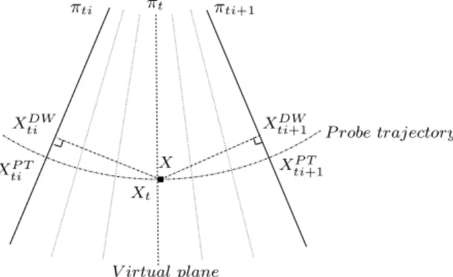
π_ti+1 X V irtual plane π_t π_ti Xt XDW ti XP T ti X P T ti+1 XDW

ti+1 _{P robe trajectory}

Fig. 1. Illustration of DW and PT principles. The two orthogonal projections for DW interpolation method and the construction of a “virtual” plane πt containing

X for PT method.

2 Method

This work builds on the distance weighted interpolation and proposes to in-corporate probe trajectory information. The distance weighted interpolation is first presented in section (2.1). Then, the probe trajectory information is incorporated in section (2.2).

2.1 Distance Weighted Interpolation (DW)

At each point X of the reconstructed volume, the linear interpolation amounts to computing: fn(X) = 1 G X ti∈Kn(X) gtif˜(Xti) (1)

where Kn is the interpolation kernel. In other words, Kn is the set of the

different indexes of the B-scans that are involved in the interpolation, n is the interpolation order. For a given interpolation degree, the n closest B-scans before X and the n closest B-B-scans after X are considered. For the DW interpolation, Xtiis the orthogonal projection of X on the tithB-scan. ˜f(Xti) is

the intensity at position Xti and is obtained by bilinear interpolation. Finally,

G is the normalization constant with G = P

gti, where gti is the distance

between X and Xti (see Fig. 1).

2.2 Probe Trajectory Interpolation (PT)

The orthogonal projection of points to the nearest B-scans is a straightforward solution. However, it does not take into account the relationship between a given point and its projections. As seen in section 1, registration based

in-terpolation uses homologous points to interpolate, thus increasing the com-putational burden. We propose to incorporate the probe trajectory into the interpolation process. In other words, homologous points are defined as being successive points along the probe trajectory.

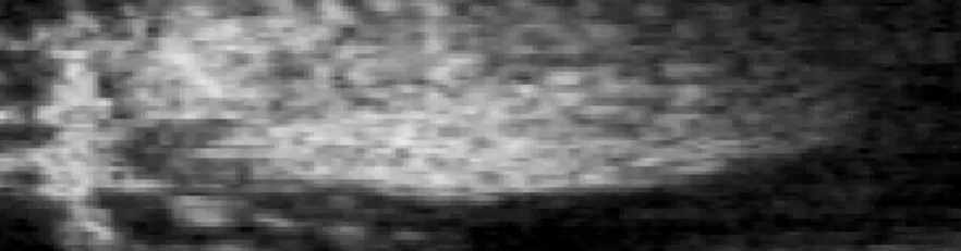
We believe there is correlation between the underlying signal structure and the probe trajectory. When imaging cross-sections of a tubular structure for instance, the intuitive displacement of the probe that follows the Structure Of Interest (SOI) will lead to some correlation between the probe trajectory and the anatomical structure (see the cerebral falx Fig. 11). In intra-operative exams, we observed that the surgeon was concentrated in keeping the focus of the US scans on the SOI (i.e. the lesion). This is confirmed by observing the location of the SOI, which is kept at the same position in the x-y place during the sequence (see Fig. 2). Therefore, we think that the introduction of probe

Fig. 2. A longitudinal reslice of the non reconstructed intra-operative data (i.e. the stack of B-scans). The x position in B-scans (horizontal axis of the reslice) of the structure of interest is correlated along the sequence, the vertical axis of the reslice corresponding to the B-scans latencies. The cerebral falx is visible at left and the lesion at center.

trajectory into the interpolation process is relevant.

Instead of using orthogonal projections as in classical DW, we propose to project along the probe trajectory. Firstly, the time stamp t ∈ R, t ∈ [ti, ti+1]

of the “virtual plane” πt is estimated. The “ virtual plane” is the plane which

passes through X in the sense of the probe trajectory (see Fig 1). Then, t is used to compute the “virtual plane” parameters (translation and rotation) by interpolation of πti and πti+1 positions. Finally, the 2D coordinates of Xt (the

projection of X on πt) are used to obtain the projections of X on πti and πti+1

in the sense of the probe trajectory.

2.2.1 Determination of the “virtual” plane time stamp

Under the assumption that the probe motion is constant between two consec-utive B-scans, the latency ratio is equal to the distance ratio:

t= dti+1 dti+ dti+1 (ti) + dti dti+ dti+1 (ti+ 1) (2)

where dti is the distance (in the sense of orthogonal projection) between the

current voxel and the B-scan of time stamp ti (dti = kX − XtiDWk). The

assumption of constant probe speed between two slices is justified by the frame rate. The lowest frame rate is usually 10Hz, which means that 100ms separate two frames. It is therefore reasonable to assume a constant motion magnitude between two frames (i.e. no significant acceleration).

Once the time stamp of the “virtual” plane is computed, the probe position can be interpolated.

2.2.2 Determination of the “virtual” plane parameters

The position of each B-scan is defined by 3 translations and 3 rotations. Thus the interpolation of origin position and rotation parameters is needed. We use the Key interpolation for the translations and the Spherical Linear Interpola-tion (SLERP) for the rotaInterpola-tions.

2.2.2.1 Interpolation of origin position For the origin of the B-scan, a cubic interpolation is used to estimate the origin of the “virtual” plane at time stamp t. The Key function is used to carry out a direct cubic interpolation and is defined as:

ϕ(t) =              (a + 2)|t|3_{− (a + 3)t}2_{+ 1 if 0 ≤ |t| < 1,}

a|t|3_{− 5at}2_{+ 8a|t| − 4a if 1 ≤ |t| < 2,}

0 if 2 ≤ |t|

(3)

With a = −1₂, ϕ is a C1 _{function and a third order interpolation is obtained}

[20]. In practice, four B-scans are used for cubic interpolation. This seems to be an optimal trade-off between computational time and reconstruction quality. For example, the interpolation of the origin position along x axis Tx reads as:

Tx(t) = ti+2 X k=ti−1 Tx(k)ϕ(t − k) (4) .

2.2.2.2 Interpolation of rotation parameters The rotation parame-ters of each B-scan are converted into a quaternion which is a compact repre-sentation of rotations within a hyper-complex number of rank 4:

This representation of rotations, allows to take into account the coupling of rotations during the interpolation step. The quaternion representing the rota-tions of the “virtual” plane is obtained through a Spherical Linear Interpola-tion (SLERP) [21] at time stamp t:

qt = qti

sin((1 − t)θ)

sinθ + qti+1

sin(tθ)

sinθ (6)

where qti and qti+1 are the unit quaternions corresponding to B-scans of time

stamps ti and ti+1; and θ represents the angle between qtiand qti+1computed

as:

θ = cos−1_(q

ti.qti+1) (7)

The orientation of the “virtual” plane is contained in qt. Then, XtiP T and Xti+1P T

are obtained directly, since they have the same 2D coordinates (defined in each B-scans) as Xt.

2.3 Labeling

It is possible that a part of the reconstructed volume is visible on several time stamps (or view points) of the B-scans sequence. These different time stamps are computed during the labeling step so as to track this information and fully exploit the speckle decorrelation. In this way, a label vector LX

containing time stamps of the nearest B-scans is built for each voxel. In case of a simple translation, LX = (t1, t1+ 1) is the label vector of voxel X while t1

and t1+ 1 are the time stamp of the nearest planes. For more complex probe

motions with multiple scanning angles, LX is composed of several couples

of time-consecutive B-scans: LX = ((t1, t1 + 1), (t2, t2 + 1), ...). Afterward,

LX is used to build Kn which also depends on interpolation degree n, thus

Kn = ((t1− n + 1, ..., t1 + n), (t2 − n + 1, ..., t2 + n), ...). For instance, with

an interpolation degree equals to 1 and two view points (see Fig. 3), the “virtual” plane between (πt1, πt1+1) is first computed to estimate the distance

of X to (πt1, πt1+1). Then, the “virtual” plane between (πt2, πt2+1) is computed

to estimate the distance of X to (πt2, πt2+1). Indeed, all the positions of the

nearest B-scans are not used at the same time to estimate the probe trajectory, only the consecutive B-scans in time are used simultaneously. Nonetheless, all the pixels on the nearest B-scans are used simultaneously to estimated the intensity of voxel X.

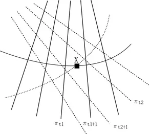
Fig. 3. Illustration of a multi-scanned voxel X at two different time stamps t1 and t2. For an interpolation degree equals to 1, the two couples of B-scans

(πt1, πt1+1) and (πt2, πt2+1) are taken into account to evaluate the intensity of X

(i.e Kn= ((t1, t1+ 1), (t2, t2+ 1)))

. 3 Material

3.1 Ultrasound Phantom sequences

A Sonosite system with a cranial 7 − 4M Hz probe was used to acquire the ultrasound images. The positions of the B-scans was given by a magnetic miniBIRD system (Ascension Technology Corporation) mounted on the US probe. The StradX software [10] was used to acquire images and 3D posi-tion data. The phantom is a CIRS Inc.1 _{3D ultrasound calibration phantom}

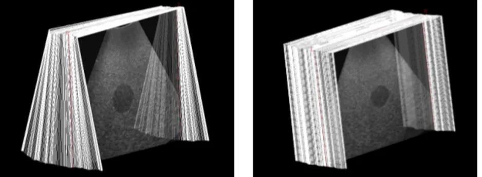
containing two calibrated volumetric ellipsoids test objects. At the acquisi-tion depth, only one of the ellipsoids is visible in the field of view. The two sequences used for the experiments are composed of 510 × 441 B-scans (204 B-scans for fan motion and 222 B-scans for translation motion, see Fig. 4).

3.2 Ultrasound Intra-operative sequences

For intra-operative sequences the sinuosity cranial probe was coupled with the Sononav Medtronic system in an image-guided neurosurgery context. Contrary to the miniBIRD tracker, the Sononav system is based on an optical tracking to estimate the spatial probe positions sent to the neuronavigation system. The sequences were acquired during neurosurgical procedures after the craniotomy

Fig. 4. B-scans sequences used during evaluation. Left: fan sequence. Right: trans-lation sequence.

step but before opening the dura. US-sequence1 is composed of 59 B-scans (223 × 405) and US-sequence2 of 46 B-scans (223 × 405), see Fig. 5.

3.3 Magnetic Resonance Intra-operative sequences

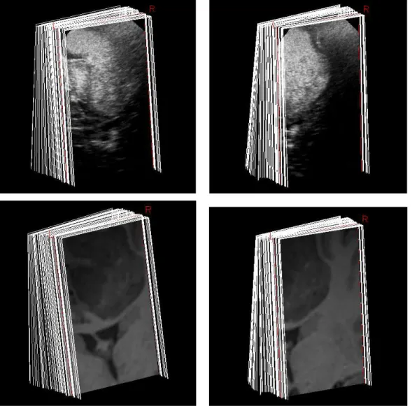
In freehand ultrasound imaging the validation step is not an easy task because the “ground truth” does not exist. In order to overcome this problem, magnetic resonance sequences were built on geometry of the ultrasonic intra-operative sequences (see Fig. 5 at bottom). Firstly, the intra operative trajectories were used to re-slice the preoperative magnetic resonance volume of the patient. Then, a stack of MR-scans was built on the images obtained by the re-slicing. Finally, the reconstructed MR volume was compared to the “ground truth” (i.e the corresponding preoperative MRI volume). As the US-sequences, the MR-sequence1 is composed of 59 MR-scans (223 × 405) and MR-sequence2 of 46 MR-scans (223 × 405), see Fig. 5.

The following evaluation aims at studying the impact of the probe trajectory incorporation independently of the compounding, the sequences follow simple fan and/or translation motion.

4 Evaluation framework

The performance of the proposed method was compared with two other in-terpolation approaches: the VNN technique used in StackX [10] and the DW method presented in [14]. For the VNN method, each voxel is projected on the nearest B-scan and its luminance interpolated bilinearly. In the DW tech-nique, each voxel is projected orthogonally on the 2n nearest B-scans and its luminance is interpolated (see section 2.1 and Fig. 1).

stud-Fig. 5. Top: Intra-operative B-scans sequences of brain used during evaluation. The low-grade glioma and ventricles are visible in white. Left: US-sequence1. Right: US-sequence2. Bottom: Intra-operative MR-scans sequences of brain built on B-s-cans sequences. Left: MR-sequence1. Right: MR-sequence2. In MR images the low– grade glioma and the ventricles appears in gray.

ied:

• “The distance between two consecutive B-sans”. The sequence is sub-sampled thanks to SelectSX2_{, which simulates a lower frame acquisition rate, in}

or-der to artificially increase the distance between 2 consecutive B-scans. The evaluation framework studies the probe trajectory interpolation impact ac-cording to the distance between two consecutive B-scans.

• “The size of the interpolation kernel”. For ultrasound phantom sequences, the removed B-scans are reconstructed with different methods and different interpolation degrees (from 1 to 2 for DW and PT methods).

4.1 For Ultrasound Phantom Data

To assess the reconstruction quality, evaluation data can be created from any image sequence: given a sequence of 3D freehand US, each B-scan is removed from the sequence, and then reconstructed by using the other B-scans. This “leave one out” procedure is performed for each B-scan. The Mean Square Error (MSE) is used as quality criterion:

M SE(t) = 1 P P X j=1 ( ˜It(xj) − It(xj))2 (8)

where It is the original image at time t (removed from the sequence), ˜It the

reconstructed image and P is the number of pixel in this B-scan. After M SE estimation for all B-scans of the sequence, we compute the mean µ and the standard deviation σ of the reconstruction error.

µ= 1 N − 2n N −n X t=n+1 M SE(t) (9) σ2 = 1 N − 2n N −n X t=n+1 (M SE(t) − µ)2 ₍₁₀₎

N is the total number of B-scan in the sequence and n the interpolation kernel degree.

4.2 For Magnetic Resonance Sequences

Contrary to ultrasound phantom data, for MR-sequences the “ground truth” is known. The evaluation framework directly compares the reconstructed volume

˜

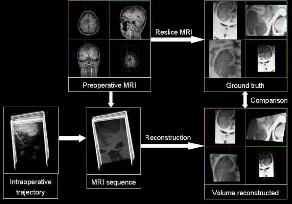
V and the corresponding volume V in preoperative MRI. Firstly, the MR sequence, obtained by reslicing the pre-operative MRI accordingly to the US trajectory, was reconstructed with the three evaluated methods. Secondly, the corresponding MR volume V (in terms of field of view and resolution) was computed using cubic interpolation. Finally, the reconstructed volumes obtained with VNN, DW and PT were compared to the “ground truth” V (see Fig. 6). The MSE between V and ˜V, obtained with the different methods, was evaluated after removing the background (i.e. voxels zero intensity). The transformation matrix given by the neuronavigator is used to register the US and MR images. This registration is not corrected with an external registration procedure since only the intra-operative trajectory is required and used to create the stack of MR-scans. This means that tracking and calibration errors are removed : therefore reconstruction errors can be studied independently of other sources of errors.

Fig. 6. Illustration of the validation framework used for the MR-sequences.

5 Results

The reconstructions were performed on a P4 3.2 Ghz with 2Go RAM. In order to only compare interpolation times, the total computational time is divided as follows: Ltime corresponds to labeling step and Itime corresponds to

interpolation time. The labeling step consists in constructing the label vector Kn for each voxel X (described in 2.3).

5.1 Interpolation Function

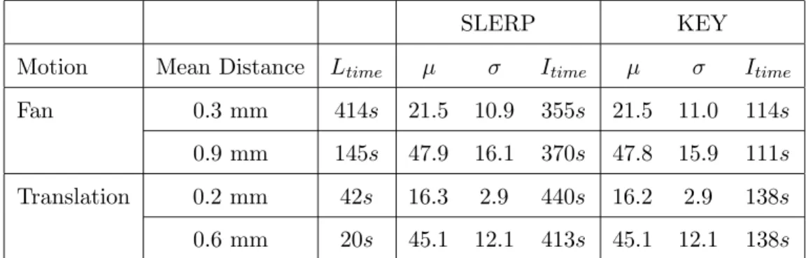
In this section, the Key interpolation of rotation parameters is compared with the theoretically optimal approach described in paragraph 2.2.2.2. The direct interpolation of each parameter can be considered as an approximation of the Spherical Linear Interpolation (SLERP) because the coupling of rotations is not taken into account. However, for small rotations, this approximation leads to very similar results. Table 1 compares the reconstruction quality using the SLERP and interpolation approximation. The SLERP interpolation is theoretically correct, but experiments showed that reconstruction results are similar. This is due to the continuity of probe motion and the proximity of two consecutive B-scans. Considering these results, the Key interpolation will be

used in the rest of the paper in order to decrease the computational burden.

SLERP KEY

Motion Mean Distance Ltime µ σ Itime µ σ Itime

Fan 0.3 mm 414s 21.5 10.9 355s 21.5 11.0 114s

0.9 mm 145s 47.9 16.1 370s 47.8 15.9 111s Translation 0.2 mm 42s 16.3 2.9 440s 16.2 2.9 138s 0.6 mm 20s 45.1 12.1 413s 45.1 12.1 138s Table 1

Error measures composed of mean µ and standard deviation σ for the Spherical Linear Interpolation (SLERP) and the Key interpolation. Results on phantom se-quence indicate that the improvement in terms of interpolation quality with SLERP was not significant whereas the computational time increased.

5.2 Phantom sequence 0.2 0.4 0.6 0.8 1 1.2 1.4 1.6 1.8 20 40 60 80 100 120 140 160

Mean distance between B−scans in mm

µ

µ for fan sequence VNN DW PT 0.2 0.4 0.6 0.8 1 1.2 0 20 40 60 80 100 120 140 160

Mean distance between B−scans in mm

µ

µ for translation sequence VNN

DW PT

Fig. 7. Variation of error reconstruction relatively to distance between two consec-utive B-scans on phantom sequence with interpolation degree equals to 1. Left fan motion, right translation motion. Three methods are evaluated: VNN, DW and PT. The PT method outperforms others methods especially on sparse data.

Results on phantom sequences (described in section 3) are presented in Figure 7 and Table 2. Figure 7 shows the influence of the mean distance between two B-scans on the reconstruction error with two types of motion (i.e. translation and fan). Table 2 presents the error and computation time for different inter-polation degrees (1 and 2). In all cases, the PT method outperforms the VNN and the DW methods especially on sequences with few B-scans. The probe trajectory is especially relevant to compensate for the sparsity of data. When the distance of a given point to the B-scans considered in the interpolation increases, the orthogonal projections and probe trajectory differ significantly. This distance introduces artifacts for the DW method. For distances close to 0.2mm, DW and PT methods are equivalent. The difference between PT

Motion Distance Interpolation VNN DW PT between

B-scans

degree µ σ Itime µ σ Itime µ σ Itime

Fan Ltime = 414s 0.3 mm n = 1 33.4 13.5 20s 22.6 11.6 44s 21.5 11.0 114s n = 2 26.2 12.5 46s 22.9 10.6 122s Ltime = 215s 0.6 mm n = 1 60.7 21.6 21s 41.1 16.9 31s 33.0 14.2 114s n = 2 46.6 17.6 44s 38.2 14.1 124s Ltime = 145s 0.9 mm n = 1 89.4 25.2 20s 61.3 19.4 30s 47.8 15.9 111s n = 2 67.6 18.6 43s 56.2 14.2 118s Translation Ltime = 42s 0.2 mm n = 1 28.2 9.6 20s 15.9 4.8 37s 16.2 2.9 138s n = 2 19.1 6.4 49s 18.3 3.5 149s Ltime = 27s 0.4 mm n = 1 60.6 22.9 21s 36.3 13.9 32s 29.3 8.6 138s n = 2 43.0 14.5 47s 35.8 8.7 147s Ltime = 20s 0.6 mm n = 1 89.3 29.6 20s 57.1 18.3 31s 45.1 12.1 138s n = 2 63.7 17.5 46s 52.9 11.1 146s Table 2

Error measures composed of mean square error µ and standard deviation σ for the different methods (see section 4). Ltime is the time spent for labeling, while Itime

is the time spent for interpolation. Results indicate that the PT method obtains better results than the VNN and the DW methods. The improvement in terms of reconstruction quality is obtained at the expense of a slight computational increase.

and DW, in terms of mean square error for translation and fan motion was expected to be greater. We think that the phantom images do not contain enough structures to really show the reconstruction quality improvement in case of fan motion. Apart from the ellipsoid in the image center, the image contains only speckle. For the fan sequence, the difference between PT and DW, in terms of projection, is substantial for voxels that are far from the rotation center, that is to say in deep areas. The deep regions do not convey structural information but mostly speckle.

Initial image VNN DW PT

Fig. 8. Differences between original (left) and reconstructed B-scan for fan sequence with n = 1. From left to right: the Voxel Nearest Neighbor, the Distance Weighted interpolation and the Probe Trajectory methods. This shows that the error between the reconstructed B-scan and the initial image is visually lower with the PT method, especially on the contours of the object.

Figure 8 shows the differences between the original and the reconstructed B-scans with the VNN, DW and PT methods. Visually, the PT reconstruction appears closer to the original B-scan, what fits the numerical results of Table

2.

5.3 MR Intra-operative sequences

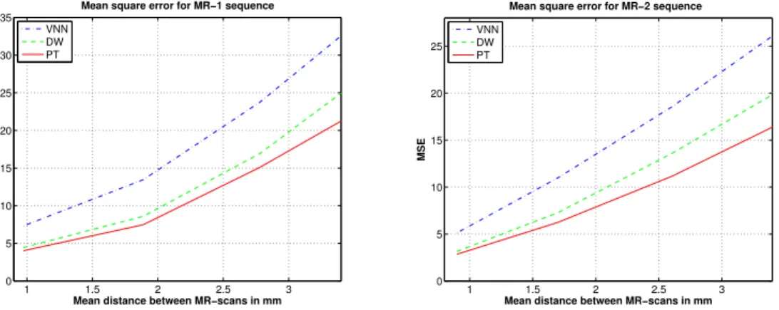
Figure 9 shows the influence of the mean distance between two consecutive B-scans on the reconstruction error. The mean square error is computed be-tween the “Ground Truth” and the reconstructed volume. The PT method outperforms the VNN and DW approaches especially on sparse data. Figure 10 presents slices extracted from initial MR volume and the reconstructed MR volume. Visually, the PT method preserves more the edges and the contrast. Compared to DW method, the PT method improves the reconstruction result especially on edges whose direction is correlated with probe trajectory.

1 1.5 2 2.5 3 0 5 10 15 20 25 30 35

Mean distance between MR−scans in mm

MSE

Mean square error for MR−1 sequence VNN DW PT 1 1.5 2 2.5 3 0 5 10 15 20 25

Mean square error for MR−2 sequence

Mean distance between MR−scans in mm

MSE

VNN DW PT

Fig. 9. Variation of mean reconstruction error relatively to the distance between two consecutive MR-scans with interpolation degree of 1. Left MR-sequence1, right MR-sequence2. Three methods are evaluated: VNN, DW and PT. The PT method outperforms others methods especially on sparse data.

5.4 US Intra-operative sequences

The dimension of the reconstructed volume are 263 × 447 × 306 for

US-sequence1 and 286×447×234 for US-sequence2 with resolutions of (0.188, 0.172, 0.180). The reconstruction process, with a multithreading implementation on an

In-tel Pentium Dual Core CPU at 3.40GHz with 2Go RAM, takes 220s for US-sequence1 and 154s for US-sequence2.

The reconstructions of B-scans dataset US-sequence1 are presented in Figure 11 and US-sequence2 are presented in Figure 12. Visually, the VNN method leads to many discontinuities and creates artificial boundaries (see image at the top right of Fig. 12). The DW method generally smooths out the edges and spoils the native texture pattern of US image more than PT (see at the bottom of Fig. 12).

“Ground truth”

VNN DW PT

Fig. 10. Results for MR-sequences of brain. Top: the “ground truth” and the recon-structions obtained via the different methods for a mean distance between MR-scans of 1.8mm. On the bottom: the images of the difference between the “ground truth” and the reconstructed volume. Visually, the PT method preserves more the edge continuity and the contrast. The difference images show that the PT method cre-ates less artifacts and appears closer to the “ground truth”, especially on ventricles edges.

The actual implementation of methods can be largely optimized as compared to StackSX, which produces all reconstruction processes of translation phan-tom sequence in 10 seconds with the VNN method (62s with our implementa-tion of VNN). Although the labeling step needs significant improvement, this

MRI VNN

DW PT

Fig. 11. Results for US-sequence1 of brain. Top: the preoperative MRI and the US reconstruction obtained with the VNN method. On the bottom: the reconstruction obtained with DW and PT approaches. The low-grade glioma and the cerebral falx appear in gray in MR image and in white in US images. From left to right the VNN, DW and PT methods. The images highlight the inherent artifacts of VNN (i.e. discontinuities) and DW (i.e. blur) methods. These results underline that the PT method preserves the edges continuity and the native texture of US image more than VNN and DW method.

study aims to compare computation time between identical implementations of methods. The increased quality of reconstruction for the PT method is ob-tained at the expense of a slight increase of the computation time. Nonetheless this side effect seems to be reasonable with regards to the reconstruction

qual-MRI VNN

DW PT

Fig. 12. Results for US-sequence2 of brain. Top: the preoperative MRI and the US reconstruction obtained with the VNN method. On the bottom: the reconstruction obtained with DW and PT approaches. The low-grade glioma appears in gray in MR image and in white in US images. Visually, the PT method preserves more the edges continuity especially on sulci edges (see at the center bottom of images).

ity. Contrary to more elaborated techniques like non-rigid registration or RBF, which are considerably computationally expensive, the PT approach offers an attractive compromise between computation time and reconstruction quality.

6 Discussion and conclusion

This paper presented a 3D freehand ultrasound reconstruction method explic-itly taking into account the probe trajectory information. Through an evalua-tion framework, it shows that the proposed method performs better than tra-ditional reconstruction approaches (i.e. Voxel Nearest Neighbor and Distance Weighted interpolation) with a reasonable increase of the computation time. The main limitation of PT method is the assumption of constant probe speed between two slices. Nonetheless, this hypothesis is reasonable when using a

decent frame rate (more than 10Hz). Moreover, the direct interpolation of ro-tation parameters instead of Spherical Linear Interpolation (SLERP) does not introduce artifacts but accelerates the reconstruction process. The evaluation results underline the relevance of probe trajectory information, especially on sequences with low frame rate acquisitions or large distances between two con-secutive B-scans. The PT method is a trade-off between reconstruction error and computational time. The results show that the hypothesis of a correlation between the signal structure and the probe trajectory is relevant. Indeed, in practice, the probe trajectory and signal structure are correlated because the medical practitioner tends to follow the structure of interest (see on Fig. 11). The precise localization of anatomy and pathology within the complex 3D geometry of the brain remains one of the major difficulties of neurosurgery. Thus, image-guided neurosurgery (IGNS) is an adequate context to exper-iment the proposed method because the reconstruction quality is of utmost importance and the time dedicated to image reconstruction is limited. The PT method is thus interesting for applications where an accurate reconstruction is needed in a reasonable time. Further work should be pursued for compar-ing the PT reconstruction approach with registration based approaches [17]. Registration based approaches avoid artifacts of slice misregistration due to errors in tracking data (i.e. trajectory) and/or tissue deformation. The com-pensation of tissue motion can be especially interesting in neurosurgery due to the complex problem of soft tissue deformations also known as brainshift. However, since the registration is a computationally expensive process, the benefit for image reconstruction should be studied. Then, our implementation could be largely optimized using graphic library implementation (ex: OpenGL) or grid computation especially for IGNS purpose. Finally, the impact of PT reconstruction on registration (mono and multimodal) to compensate for er-rors of localization and brainshift needs to be investigated further. Indeed, the current pitfalls of the neuronavigator system are: the errors caused by geomet-rical distortion in the preoperative images, registration, tracking errors [22], and brainshift.

Acknowledgment

We thank Richard Prager, A. Gee and G. Treece from Cambridge Univ. for fruitful assistance in using StradX. This work was possible thanks to a grant of Rennes city council. We thank the reviewers for their valuable comments for improving this paper.

References

[1] J. M. Rubin, M. Mirfakhraee, E. E. Duda, G. J. Dohrmann, F. Brown, Intraoperative ultrasound examination of the brain, Radiology 137 (3) (1980) 831–832.

[2] G. J. Dohrmann, J. M. Rubin, History of intraoperative ultrasound in neurosurgery, Neurosurgery Clinics of North America 12 (1) (2001) 155–166. [3] R. N. Rankin, A. Fenster, D. B. Downey, P. L. Munk, M. F. Levin,

A. D. Vellet, Three-dimensional sonographic reconstruction: techniques and diagnostic applications, American Journal of Roentgenology 161 (4) (1993) 695– 702.

[4] S. W. Smith, R. E. Davidsen, C. D. Emery, R. L. Goldberg, E. D. Light., Update on 2-D array transducers for medical ultrasound, in: Proceeding IEEE Ultrasonics Symposium, 1995, pp. 1273–1278.

[5] S. W. Smith, K. Chu, S. F. Idriss, N. M. Ivancevich, E. D. Light, P. D. Wolf, Feasibility study : real-time 3-D ultrasound imaging of the brain, Ultrasound in Medicine and Biology 30 (10) (2004) 1365–1371.

[6] R. San-Jose, M. Martin-Fernandez, P. P. Caballero-Martinez, C. Alberola-Lopez, J. Ruiz-Alzola, A theoretical framework to three-dimensional ultrasound reconstruction from irregularly-sample data, Ultrasound in Medicine and Biology 29 (2) (2003) 255–269.

[7] F. Rousseau, P. Hellier, C. Barillot, Confhusius: a robust and fully automatic calibration method for 3D freehand ultrasound, Medical Image Analysis 9 (2005) 25–38.

[8] F. Rousseau, P. Hellier, C. Barillot, A novel temporal calibration method for 3-d ultrasound, IEEE Transactions on Medical Imaging 25 (8) (2006) 1108–1112. [9] L. Mercier, T. Lango, F. Lindseth, L. D. Collins, A review of calibration

techniques for freehand 3-D ultrasound systems, Ultrasound in Medicine and Biology 31 (2) (2005) 143–165.

[10] R. W. Prager, A. H. Gee, L. Berman, Stradx : real-time acquisition and visualization of freehand three-dimensional ultrasound, Medical Image Analysis 3 (2) (1999) 129–40.

[11] T. R. Nelson, D. H. Pretorius, Interactive acquisition, analysis and visualization of sonographic volume data, International Journal of Imaging Systems and Technology 8 (1997) 26–37.

[12] S. Sherebrin, A. Fenster, R. N. Rankin, D. Spence, Freehand three-dimensional ultrasound: implementation and applications, in: Proc. SPIE Vol. 2708, p. 296-303, Medical Imaging 1996: Physics of Medical Imaging, Richard L. Van Metter; Jacob Beutel; Eds., 1996, pp. 296–303.

[13] C. D. Barry, C. P. Allott, N. W. John, P. M. Mellor, P. A. Arundel, D. S. Thomson, J. C. Waterton, Three dimensional freehand ultrasound: image reconstruction and volume analysis, Ultrasound in Medicine and Biology 23 (8) (1997) 1209–1224.

[14] J. W. Trobaugh, D. J. Trobaugh, W. D. Richard, Three dimensional imaging with stereotactic ultrasonography, Computerized Medical Imaging and Graphics 18 (5) (1994) 315–323.

[15] R. Rohling, A. H. Gee, L. H. Berman, G. M. Treece, Radial basis function interpolation for freehand 3D ultrasound, in: A. Kuba, M. S´amal, A. Todd-Pokropek (Eds.), Information Processing in Medical Imaging, Vol. 1613 of LNCS, Springer, 1999, pp. 478–483.

[16] R. Rohling, A. Gee, L. Berman, A comparison of freehand three-dimensional ultrasound reconstruction techniques, Medical Image Analysis 3 (4) (1999) 339– 359.

[17] G. P. Penney, J. A. Schnabel, D. Rueckert, M. A. Viergever, W. J. Niessen, Registration-based interpolation, IEEE Transactions on Medical Imaging 23 (7) (2004) 922–926.

[18] S. Meairs, J. Beyer, M. Hennerici, Reconstruction and visualization of irregularity sampled three- and four-dimensional ultrasound data for cerebrovascular applications, Ultrasound in Medicine and Biology 26 (2) (2000) 263–272.

[19] J. M. Sanchez, J. S. Marques, A rayleigh reconstruction/interpolation algorithm for 3D ultrasound, Pattern recognition letters 21 (10) (2000) 917–926.

[20] P. Th´evenaz, T. Blu, M. Unser, Interpolation revisited, IEEE Transactions on Medical Imaging 19 (7) (2000) 739–758.

[21] K. Shoemake, Animating rotation with quaternion curves, in: SIGGRAPH ’85: Proceedings of the 12th annual conference on Computer graphics and interactive techniques, ACM Press, New York, NY, USA, 1985, pp. 245–254.

[22] J. G. Golfinos, B. C. Fitzpatrick, L. R. Smith, R. F. Spetzler, Clinical use of a frameless stereotactic arm: results of 325 cases, Journal of Neurosurgery 83 (2) (1995) 197–205.