HAL Id: hal-00909513
https://hal.archives-ouvertes.fr/hal-00909513
Submitted on 26 Nov 2013HAL is a multi-disciplinary open access archive for the deposit and dissemination of sci-entific research documents, whether they are pub-lished or not. The documents may come from teaching and research institutions in France or abroad, or from public or private research centers.
L’archive ouverte pluridisciplinaire HAL, est destinée au dépôt et à la diffusion de documents scientifiques de niveau recherche, publiés ou non, émanant des établissements d’enseignement et de recherche français ou étrangers, des laboratoires publics ou privés.
Efficiency Improvement of Measurement Pose Selection
Techniques in Robot Calibration
Yier Wu, Alexandr Klimchik, Anatol Pashkevich, Stéphane Caro, Benoît Furet
To cite this version:
Yier Wu, Alexandr Klimchik, Anatol Pashkevich, Stéphane Caro, Benoît Furet. Efficiency Improve-ment of MeasureImprove-ment Pose Selection Techniques in Robot Calibration. The IFAC Conference on Manufacturing Modeling, Management and Control (MIM 2013), Jun 2013, Saint Petersburg, Russia. pp.832-837. �hal-00909513�
Y.Wu1,2, A. Klimchik1,2, A. Pashkevich1,2, S.Caro2, B.Furet3
1
Ecole des Mines de Nantes,44307, Nantes, France
2
Institut de Recherche en Communications et Cybernétique de Nantes (IRCCyN), 44321, Nantes, France
3
Université de Nantes, 44322, Nantes, France
(e-mail:{ yier.wu, alexandr,klimchik, anatol,pashkevich} @mines-nantes.fr, [email protected], [email protected])
Abstract: The paper deals with the design of experiments for manipulator geometric and elastostatic
cal-ibration based on the test-pose approach. The main attention is paid to the efficiency improvement of numerical techniques employed in the selection of optimal measurement poses for calibration experi-ments. The advantages of the developed technique are illustrated by simulation examples that deal with the geometric calibration of the industrial robot of serial architecture.
Keywords: robot calibration, measurement pose selection, test-pose approach
1. INTRODUCTION
In the usual engineering practice, the accuracy of a manipula-tor depends on a number of facmanipula-tors. Usually in robotics, the geometric and elastostatic errors are the most significant ones. Their influence on the robot positioning accuracy highly depends on the manipulator configuration and essen-tially differs throughout the workspace. To achieve good ac-curacy in all working points, adequate geometric and stiff-ness models are required. While the model structure is usu-ally well known, the identification of the model parameters (calibration) is rather time consuming and requires essential experimental work. For this reason, optimal selection of measurement poses for robot calibration is an important prob-lem, which is still in the focus of numerous research papers (Daney 2002, Sun 2008).
At present, the main activity in this area is concentrated around the geometric calibration (Khalil 2002). On the other hand, the elastostatic calibration which is also very important for many applications (such as precise machining) has at-tracted less attention of the researchers (Meggiolaro 2005). However, for both of these calibration procedures, the prob-lem of measurement pose selection is one of the key issues allowing to reduce essentially the measurement error impact (Klimchik 2011). At first sight, this problem can be solved using well known results from the classical design of experi-ments theory. However, because of the specificity and nonlinearity of the manipulator geometric and elastostatic models, the problem solution is not so obvious. The main difficulties here are in the area of definition of a reasonable optimality criterion (which has clear engineering sense) and also in efficient solution of the relevant optimization prob-lem, which has rather high dimension.
Among related works, it is worth mentioning several papers. The majority of the measurement pose selection techniques
relies on the optimization of some functions depending on the singular values of the identification Jacobian. For example, Zhuang used genetic algorithm for minimization of the condi-tion number of this matrix (Zhuang 1996). In other work (Daney 2005), to decrease the sensitivity to local minima, Daney developed the local convergence method and Tabu search technique based on the observability index. However, the performance measures used in these works are rather ab-stract and are not directly related to the robot accuracy. Be-sides, the related objective functions are very difficult for the optimization due to existence of a number of local minima. To find the global one, heuristic search is usually used as the numerical algorithms, which often require tedious computa-tions. All these motivate the research direction of this work. In this paper, the problem of optimal design of calibration experiments is studied for the case of robot manipulator of serial architecture. In contrast to other works, the optimiza-tion problem related to measurement pose selecoptimiza-tion is formu-lated using the proposed performance measure (test-pose approach), which has clear physical meaning and is directly related to robot accuracy. The main attention is paid to the efficiency improvement of the related numerical routines.
2. PROBLEM STATEMENT
2.1 Geometric and Elastostatic Models of Manipulator In industrial robot controllers, the end-effector position of the manipulator is usually computed using the geometric model. For some specific applications, such as high-speed machining that generate essential external loading, the elastostatic model should be also used. However, in practice, the robot geomet-ric parameters essentially differ from the nominal values de-clared in technical specifications and vary from one robot to another. In addition, elastostatic parameters of the manipula-tor are not provided by the robot manufacturers and can be identified from the experiments only. So, the manipulator
model parameter identification is an important step in practi-cal application of industrial robots.
The manipulator geometric model provides the posi-tion/orientation of robot end-effector as a function of the joint variables and its inherent parameters. This model is usually presented as a product of homogeneous transformation matri-ces, which after some transformations can be presented as the vector function
,g
p q П
(1)where vector denotes the end-effector position, vector aggregates all joint angles and Пare the vector of unknown parameters to be identified. These unknowns differ with the applied parameterization methods in robot geometric model-ling, such as the classical Denavit and Hartenberg approach and its modified version (Khalil 1986). In this paper, there are considered the most essential components of the vector
, which are the deviations of the robot link lengths i
p q
П l and
the offsets i in the actuated joints. Since the deviations of
geometrical parameters are usually relatively small, calibration usually relies on the linearized model
q П
, 0
g
, 0
g p q П J q П П / p
(2) which includes the conventional geometric Jacobiancomputed for the nominal geo-metric parameters
.
0 0 , , g q П g q П J Π 0 ПThe elastostatic properties of a serial robotic manipulator represent its resistance to deformations caused by external forces/torques and are usually described by the Cartesian stiffness matrix KC, which is computed as
1 C θ θ θ T K J K J (3)
where θ is a diagonal matrix that aggregates the joint stiff-ness values (that are the unknowns to be identified) and θ is the corresponding elastostatic Jacobian. This model can be derived using the virtual joint method, which describes all elastostatic properties of compliant elements by localized virtual springs located in the actuated joints (Salisbury 1980). Using the Cartesian stiffness matrix, the elastostatic model (or force-deflection relation) can be expressed as
K J 1 θT θ θ J J w K (4)
where is the position deflection at the robot end-effector caused by the external wrench w , which integrates both the external force and torque. This linear relation can be further used for the calibration where the desired parameters to be identified are the components of matrix .
p
θ K
In the frame of this work, several assumptions concerning calibration of these models are accepted:
A1: For the geometric calibration, each calibration
experi-ment produces two vectors
i i , which define the robot end-effector displacements and corresponding joint angles., p q
The linear relation between the errors in geometric parame-ters and the end-effector position deviations can be written as
= ( )
i g i
p J q Π (5)
where J qg( )i is the Jacobian matrix that depends on ma-nipulator configuration qi and vector collects the un-known parameters to be identified.
Π
A2: For the elastostatic calibration, each calibration
experi-ment produces three vectors , where defines the applied forces and torques.
, ,
i i i
p q w wi
In accordance with (Pashkevich 2011), the corresponding mapping from the external wrench space to the end-effector deflection space can be expressed as
θ θ θ
= ( ) T( )
i i i
p J q k J q wi (6)
where θis a matrix that aggregates the unknown compliance parameters
k
k1,...,kn
to be identified.Hence, the calibration experiments provide the set of vectors
p q and i, i
p q w that allow us to estimate the de-i, i, i
viations in geometric parameters (compared to the nomi-nal values) and absolute values of the elastostatic parameters included in the diagonal matrix k .П
θ
2.2 Identification of the Model Parameters
The problem of parameter identification of the robot manipu-lator can be treated as the best fitting of the experimental data by corresponding models. These data are measured under several assumptions concerning the measurement equipment:
A3: The calibration relies on the measurements of the
end-effector position only (Cartesian coordinates
p px, y,pz
).A4: The measurements errors
i accommodated in each
measurement of end-effector position are treated as inde-pendent identically distributed random values with zero ex-pectation and standard deviation
ε
.
For computational convenience and taking into account the influence of measurement errors, the geometric and elas-tostatic models described by separate linear equations (5) and (6) can be expressed in the following integrated form
( )
i i i
p B q X ε (7)
where X
Π k collects all unknown parameters (both ,
geometric and elastostatic ones), and the matrix B varies depending on different calibration cases
3 3 3 2 3 3 2 3 3 2 3, for geometric parameters , for elastostatic parameters , for both parameters
m n m n m n m n m n m n m n J 0 B 0 A J A (8)
where is the Jacobian matrix that can be obtained by differ-entiating the manipulator geometric model with respect to the desired parameters; and matrix A can be computed as
J
1 1
( ,i i) J ( i)JT( i) i,...,Jn( i) nT( i) i
A q w q q w q J q w (9)
where is the column vector of the Jacobian ma-trix for the experiment. is the number of joints.
( i) n J q -th i -th n n
Using usual approach adopted in the identification theory, the estimated unknown parameters can be ob-tained using the least square method, which yields
θ ˆ ˆ ˆ, X Π k
1 1 1 ˆ T · T i i i i m m i i X
B B
B p (10)Using this expression, it can be proved that the covariance matrix for the identification errors in the parameters X can be computed as 1 2 1 ˆ cov( ) m T i i i
X B B (11)where is the standard deviation (s.t.d.)of the measurement errors. Hence, the impact of the measurement errors on the parameter identification accuracy is defined by the matrix sum
mi1 T that is also called the information matrix.i i
B B
It is obvious that, from practical point of view, the covariance matrix should be as small as possible. However, strict mathematical definition of this notion is not trivial and a number of different approaches are proposed in literature. In most of the related works, the optimal measurement poses are obtained based on minimization of the covariance matrix norm (Atkinson 1992). This approach may provide a solu-tion, which does not guarantee the best position accuracy for typical manipulator configurations defined by the manufac-turing process. Thus, here it is proposed the industry-oriented performance measure, 2
0
, which is defined as the mean square error in the end-effector position after compensation. To develop this approach, let us introduce several definitions:
D1: Plan of experiments is a set of robot configurations
and corresponding external loadings W that are used for the measurements of the end-effector displacements and fur-ther identification of the desired parameters.
Q
D2. The accuracy of the error compensation
0
is the dis-tance between the desired end-effector position and its real position achieved after application of error compensation technique.
D3. The manipulator test-pose is one or set of robot
configu-rations 0 and corresponding external loadings W0 for
which it is required to achieve the best error compensation (i.e. ). Q mi 2 0 n
In the frame of the adopted notations, the distance defining the error compensation accuracy can be computed as
0( ˆ
p B X X) (12)
where the vectors and are the true parameters val-ues and their estimates, respectively. Matrix B0 corresponds to the test pose (see expressions (8)). Further, taking into ac-count that
X Xˆ
p
, it can be easily proved that the expectation is a function of the unbiased random variables
ε1,...,εmE( p) 0. Besides, the variance can be expressed as
T T
0 0 Var(p)E X B BX 0 T (13)where is the difference between the esti-mated and true values of the parameters. Expression. (13) can be rewritten as t 0 0 and after relevant transformations in accordance with (10), (11), yields the de-sired expression for the compensation accuracy
ˆ X X X race(B E( X X BT) T) 1 2 2 0 0 1 trace ( ) ( ) m T i i i B
B q B q B (14)As follows from this expression, the proposed performance measure can be treated as the weighted trace of the covari-ance matrix (11), where the weighting coefficients are com-puted using the test pose.
Hence, the identification quality (evaluated via the error compensation accuracy) is completely defined by the set of matrices
B1,...,Bm
that depend on the manipulator configu-rations
q1,...,qm
. Optimal selection of these configurations will be in the focus of next Subsection.2.3 Problem of the Measurement Poses Selection
Based on the performance measure presented in the previous Subsection, the corresponding optimization problem of the measurement pose selection can be defined as
1 0 , 1 trace ( ) ( ) min subject to ( , ) 0, 1, i i m T T i i i i i i i r
q w B B q B q B C q w 0 (15)Here, the matrices describe some constraints, which should be taken into account while solving optimiza-tion problem. These constraints are imposed by the work-cell design particularities and usually include the manipulator joint limits, the work-cell space limits, measurement equip-ment limitations, etc. It should be also equip-mentioned that some constraints are imposed to avoid collisions between the work-cell components and the manipulator. Besides, some direc-tions of the applied loading are preferable for the reason of practical implementation.
( , )
i i i
C q w
It should be mentioned that the component of the matrices
i vary with different calibration cases and may include
some very specific constraints. For instance, for the case of elastostatic calibration, they can be expressed as
C max min max 1 min min 3 4 min min 2 max , , C i i z z i i i i i i i q q p p q q r r F C p p C C p p F (16)
where and are the joint limits, max min
i
q max
i
q F is the robot maximum payload, is the minimum height between the end-point of the calibration tool and the work-cell floor, is the minimum radius to avoid collisions between the ap-plied loading and robot body,
min z p min r min
is the minimum angle between the direction of calibration tool and z-axis of robot base frame to ensure that the vertical loading can be applied, and are the boundaries of work-cell space. For the case of geometric calibration, the problem of applying exter-nal loading does not exist. So, C2, 3are zero matrices, while , remain the same as in elastostatic calibration.
min i p pmai 1 C C x 4 C
The procedure of solving such an optimization problem could be very tedious for the case when numerous measurement configurations are required for the calibration experiment. For this reason, the problem of interest is to find reasonable
number of different measurement configurations and to im-prove the efficiency of optimization routines employed in the measurement pose selection.
3. MEASUREMENT POSE SELECTION TECHNIQUES To solve the above define problem, several techniques can be applied. This section presents the analysis and propose some approaches allowing to obtain acceptable solution in reason-able time. The main difficulties here are related with a large number of variables and complex behaviour of the objective function that has many local minima.
3.1 Using Conventional Optimization Techniques
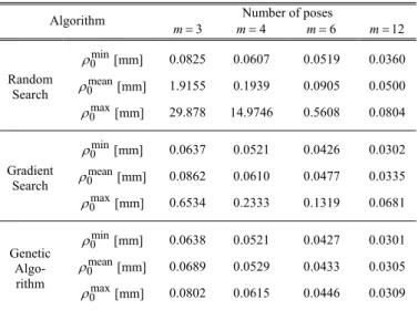
The simplest way to solve this problem is to apply conven-tional optimization techniques incorporated in commercial mathematical software. It is clear that straightforward search with regular grid is non-acceptable here because of high complexity and enormous number of solutions to be com-pared. For this reason, three other algorithms have been ex-amined: (i) random search, (ii) gradient search, and (iii) genetic algorithm. Their comparison study is presented below and summarized in Tables 1 and 2, where two criteria have been used: computational time and the ability to find optimal solution (evaluated via , the manipulator accuracy 0 after calibration). For all computational experiments, it was assumed that the s.t.d. of the measurement errors is 0.03mm. The benchmark example deals with the calibration experi-ments design for 6-dof industrial manipulator KUKA KR270, whose nominal parameters can be found on the manufacturer website (www.kuka.com). The robot has a serial architecture with six actuated revolute joints, so 24 independent geomet-ric parameters should be identified in general case. But for this example, to reduce computational efforts and evaluate the algorithm capability before applying to the problem of real dimension, only nine of the most essential parameters were identified (which have major impact on the positioning accuracy). This allowed us to obtain realistic assessments of the conventional optimization techniques capabilities with respect to the considered problem where the number of de-sign variables is high enough (72 for 12 configurations). The first of the examined algorithm (i) is based on the straightforward selection of the best solution from the set of ones generated in a random way. For this study, 10,000 solu-tions were generated for different numbers of measurement configurations . As follows from the obtained results (see Tables 1 and 2), this algorithm is very fast and requires less than 2 minutes to find the best solution. How-ever, this solution is essentially worse than the optimal one (by 15-30%).
3, 4, 6,12m
The second algorithm (ii) employs the gradient search with built-in numerical evaluation of the derivatives that is avail-able in Matlab. The starting points were generated randomly and, to avoid convergence to the local minima, the optimiza-tion search has been repeated 5000 times (starting from dif-ferent points). In this case, it has been obtained the best result in terms of the desired objective , but computational cost 0
was very high (it can overcome a hundred of hours). So, this technique is hardly acceptable in practice. It is worth men-tioning that reduction of the iteration number is rather dan-gerous here, because there are a number of local minima that the algorithm can converge to (see Table 1 that includes the minimum, maximum and average values of obtained for 0 random starting points). Moreover, as follows from our ex-perience, 5000 iterations are also not enough here.
Table 1. Efficiency of conventional optimization techniques
Number of poses Algorithm 3 m m 4 m 126 m min 0 [mm] 0.0825 0.0607 0.0519 0.0360 mean 0 [mm] 1.9155 0.1939 0.0905 0.0500 Random [m 29.878 14.9746 5608 0.0804 [mm] 0.0637 0.0521 0426 0.0302 Search max 0 m] 0. 0. min 0 mean 0 [mm] 0.0862 0.0610 0.0477 0.0335 Gradient [m 0.6534 0.2333 1319 0.0681 0.0638 0.0521 0427 0.0301 Search max 0 m] 0. 0. min 0 [mm] mean 0 [mm] 0.0689 0.0529 0.0433 0.0305 Genetic Algo-rithm max 0 [mm] 0.0802 0.0615 0.0446 0.0309
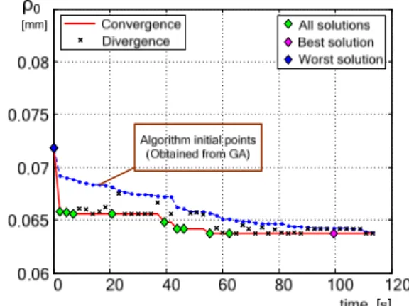
The third of the examined techniques (iii) applies genetic algorithm (GA) that is based on adaptive heuristic search. The optimization has been carried out for 100 times with population size 50 and 20 generations (initial populations were randomly generated). For illustrative purposes, Fig.1 presents the efficiency of this algorithm for selection of three optimal measurement configurations. It shows the algorithm convergence as well as divergence of the optimal solutions with respect to computing time. As follows from this figure, the optimization results are highly sensitive to the selection of initial population. In particular, the diversity of the optimal solutions got from sequential GA runs is about 25%. So, to achieve the global minimum, the GA should be repeated many times, which leads to essential increase of the computa-tional efforts (more than 6 hours of computations for the con-sidered example). However, compared to gradient search, GA provides acceptable accuracy (only 2% worse) while the computational time is 4 times less.
Table 2. Computational time of examined algorithms
Number of poses Algorithm
3
m m4 m6 m12
Random Search 41s 47s 1min 1.7min
Gradient Search 24.2h 37.5h
G
56.3h 103.6h
enetic Algorithm 6.5h 8.3h 10.5h 15.4h
As follows from the obtained results, the random search is rather fast but inefficient here, since it may produce non-acceptable solutions. In contrast, the gradient search is able to find the global minimum provided that it is repeated many times with different starting points. As a compromise, the GA
provides intermediate results in terms of accuracy and com-putational time. However, for problems of the real industrial size, the performances of the GA are also not sufficient. For this reason, the following Subsections are devoted to the im-provement of the numerical optimization techniques em-ployed in selection of optimal measurement poses.
time, [h]
Figure 1. Efficiency of GA for selection of three
measure-ires numerous repetitions
of the parallel computing, the same ment poses (population size 50, 20 generations)
3.2 Applying Parallel Computing Since the considered problem requ
of the optimization with different initial values, applying par-allel computing looks attractive to speed up the design proc-ess and to take advantage of multi-core architecture available in modern computers.
To evaluate benefits
benchmark example has been considered and two algorithms have been examined: (ii)' parallel gradient search, and (iii)' parallel GA with the same parameter settings. The computa-tions were carried out on the workstation with 12 cores. The obtained results are presented in Table 3, which gives the computational time for different number of measurement poses (the attained value of the objective function is very 0 close to those presented in Table 1).
The obtained results are quite expected and confirm essential
algorithms using
Number of poses
reduction of computational efforts. For both optimization methods, the consumed time has been decreased by the factor of 10-12 (compared to the results in Table 2). However, it is not enough yet to solve the problem of real industrial size, where several dozen of parameters should be identified (in-stead of nine in the benchmark example).
Table 3. Computational time of examined parallel computing
Algorithm
3
m m4 m6 m12
Parallel
Gradient Search 2.1h 3.2h 4.9h 8.9h
Parallel
Genetic Algorithm 36min 41min 52min 1.5h
.3 Using Hybrid Approach
h examined algorithms and 3
To take the advantages of bot
efficiency of the parallel implementation, a hybrid technique has been developed. It should be mentioned that some soft-ware packages (Matlab, etc.) already implement this idea and use the final solution from GA as the initial point of gradient search. However, since the randomly generated initial popu-lations in GA may cause high diversity of the optimal solu-tions, the selection of these initial values is also an important issue. For this reason, the embedded hybrid option in GA cannot be directly used and requires additional modifications. To improve the efficiency of the existing technique, the start-ing point selection strategy for the gradient search has been modified. To ensure better convergence to the global mini-mum, it has been proposed to use the best half of final points obtained from GA as the starting points for the gradient search. From our point of view, it ensures better diversity of the starting points and allows to avoid convergence to the local minima.
Figure 2. Efficiency of the hybrid approach for selection of
on has been evaluated using the
on of Problem Dimension
e only three measurement poses
The proposed modificati
same benchmark example. For comparison purposes, Fig 2. presents the convergence of the hybrid method for the prob-lem of optimal selection of three measurement configurations studied in the previous Subsection (see Fig. 1). It shows the initial points (obtained from GA), optimal solutions as well as the solution improvement with respect to time. As follows from the figure, the hybrid algorithm can converge much faster, but if the number of measurement poses is increased up to 12, the computational time is over 1.6 hour that is still unacceptable for industry.
3.4 New Approach: Reducti
Generally, as follows from the identification theory, th way to improve calibration accuracy is to increase the num-ber of measurements (provided that the reduction of the measurement errors is not possible). However, for the ma-nipulator calibration problem, each measurement is associ-ated with a certain robot configuration that also has influence on the final accuracy. It is clear that the best result is achieved if all measurement poses are different and have been optimized during the calibration experiment planning.
s been
tions provides almost the same performance as "full-dimensional" optimal plan. Obviously, this reduction of the measurement pose number is very attractive for the engineer-ing practice.
4. CONCLUSIONS On the other hand, as follows from our experiences, the
di-versity of the measurement poses does not contribute signifi-cantly to the accuracy improvement if m is high enough. This allows us to propose an alternative which uses the same measurement configurations several times (allowing to sim-plify and speed up the measurements). This approach will be further referred as "reduction of problem dimension".
To explain the proposed approach in more details, let us as-sume that the problem of the optimal pose selection ha solved for the number of configurations that is equal to m , and the obtained calibration plan ensures the positioning ac-curacy . Using these notations, let us evaluate the calibr -0m tion accuracy for two alternative strategies that employ larger number experiments km:
Strategy #1 (conventional): the measurement poses are found from the full-scale optim tio
a
of
iza n of size
m the low-km.
Strategy #2 (proposed): the measurement poses are obtained by simple repetition the configurations got fro
dimensional optimization problem of size m .
It is clear that the calibration accuracy for strategy #1 is 0km better than the accuracy corresponding to t e sh trategy #2 that can be expressed as 0m k . However, a follows from our study, this difference is not high if m is larger than 3. This allows us to essential e the size of optimization prob-lem employed in the optimal selectio of measurement poses without significant impact on the positioning accuracy. To demonstrate the validity of the proposed approach, the benchmark example has been solved using strategies #
s
ly reduc
n
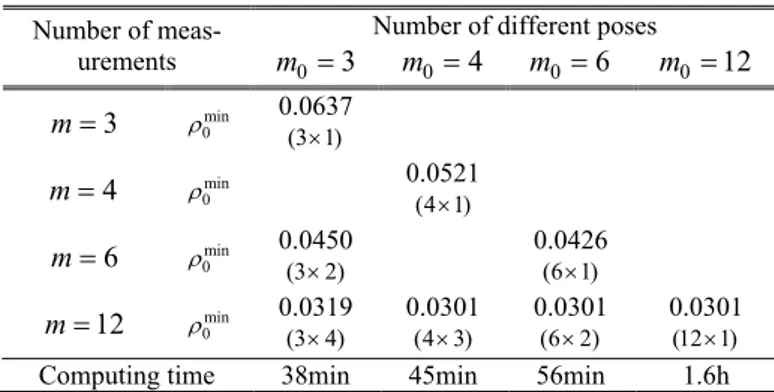
1 and #2 assuming that the total number of measurements is equal to 12 (i.e. using different factorizations such as 12 1 , 6 2 ,
4 3 , 3 4 ). Relevant results are presented in Table 4 (see the last line). As follows from them, the factorizatio n12 1
e easurement poses are different is only 6% better compared to the factorization 3 4 where measuremen repeated 4 times in 3 different configurations. At the same time the factorizations 6 2 a 3 give almost the same results as the optimal factorizations 12 1 . On the other hand, the computational time of the op l pose generation for
3
m is much lower than for m 1
wher all m
ts are
nd 4
tima
2
. This demonstrates the efficiency of the proposed approach and justify its validity. Table 4. Calibration accuracy for different factorizations 0 of the experiment number mkm0
Number of different poses Number of meas-urements m0 3 m0 4 m0 6 m0 12 3 m min 0 0.0637(3 1) 4 m min 0 0.0521(4 1) 6 m min 0 0.0450(3 2) 0.0426(6 1) 12 m min 0 0.0319(3 4) 0.0301(4 3) 0.0301(6 2) 0.0301(12 1)
Computing time 38min 45min 56min 1.6h
Hence oncl that ing ment
o tain the num con
The paper presents ptimal selection of measurement poses In contrast to other
The authors would inancial support of the French “Ag echerche”(Project
periment Designs. Oxford U xford.
152. e local Kha gs of Kha ks. Journal of Intelli-Klim ar anthropo-Meg u-Pash
with massive joints.
Sali
Sun
p.831-836.
botics and Automation, 2, pp. 981-986. a new technique for o
in robot calibration.
works, it is proposed to evaluate the quality of calibration plans via the manipulator positioning accuracy for a given test pose, and to reduce number of design variables in the related optimization problem by means of repeating meas-urements with lower number of configurations. This tech-nique allows us to essentially reduce the computational time for solving the problem of real industrial size. The advan-tages of the developed technique were confirmed by a simu-lation example, where the proposed approach permitted to decrease the computing time by more than 10 times while losing only 6% of manipulator positioning accuracy. Future work in this direction will deal with the efficiency improve-ment of the manipulator elastostatic calibration.
ACKNOWLEGMENT like to acknowledge the f
ence Nationale de la R ANR-2010-SEGI-003-02-COROUSSO), France.
REFERENCES
Atkinson, A.C., Donev, A.N., (1992). Optimal Ex niversity Press, O
Daney, D., (2002). Optimal measurement configurations for Gough platform calibration. ICRA, pp.
147-Daney, D., Papegay, Y., Madeline, B., (2005). choosing measurement poses for robot calibration with th
convergence method and tabu search. International Journal of Robotics Research, 24(6), pp. 501–518. lil W., Kleinfinger J.F., (1986). A new geometric
nota-tion for open and closed-loop robots. Proceedin ICRA Conference, pp. 1174-1180.
lil, W., Besnard, S., (2002). Geometric calibration of robots with flexible joints and lin
gent and Robotic Systems, 34, pp. 357-379.
chik, A., Wu,Y., Caro, S., Pashkevich, A., (2011). De-sign of experiments for calibration of plan
morphic manipulators. AIM Conference, pp. 576-581. giolaro, M.A., Dubowsky, S., Mavroidis, C., (2005). Geometric and elastic error calibration of a high acc racy patient positioning system. Mechanism and Ma-chine Theory, 40, pp. 415–427.
kevich A., Klimchik A., Chablat D. (2011). Enhanced stiffness modeling of manipulators
Mechanism and Machine Theory, vol. 46, pp. 662-679. sbury, J., (1980). Active stiffness control of a manipulator
in Cartesian coordinates. Proceedings of 19th IEEE Con-ference on Decision and Control, pp. 87–97.
, Y., Hollerbach M., (2008). Observability index selection for robot calibration. Robotics&Automation, p
Zhuang, H., Wu, J., Huang, W., (1996). Optimal planning of robot calibration experiments by genetic algorithms. Ro-, it can be c ptimal plans ob ude ed for d repeat lower expe ber of ri s wi figura-th