General study of single input single output linear time invariant laws. Application to an adapted models algorithm control.

HAL Id: hal-00705033

https://hal-mines-paristech.archives-ouvertes.fr/hal-00705033

Submitted on 6 Jun 2012

HAL is a multi-disciplinary open access

archive for the deposit and dissemination of

sci-entific research documents, whether they are

pub-lished or not. The documents may come from

teaching and research institutions in France or

abroad, or from public or private research centers.

L’archive ouverte pluridisciplinaire HAL, est

destinée au dépôt et à la diffusion de documents

scientifiques de niveau recherche, publiés ou non,

émanant des établissements d’enseignement et de

recherche français ou étrangers, des laboratoires

publics ou privés.

General study of single input single output linear time

invariant laws. Application to an adapted models

algorithm control.

Laurent Praly

To cite this version:

Laurent Praly. General study of single input single output linear time invariant laws. Application to

an adapted models algorithm control.. 1980. �hal-00705033�

General study of single input single output

linear time invariant laws.

Application to an adapted models algorithm control

(AMAC).

Abstract : In this study, we come back on some

charac-teristics of linear time invariant control laws and we

show how the single input single output (SISO) adapted

model algorithm control (AMAC) is a technique for

designing such a law.

June 1980

CAI Ecole des Mines de Paris,

35

Rue Saint Honore, Fontainebleau

Introduction

Let us return on what is the p r o b Lc rn of sampled-data control systems synthesis.

Given a mathematical model of a process, functionnal operator between an input and an output, given a set of

specifications, given a method to compute a control input, the problem of synthesis may be defined as follows : find the parameters used in the computation of the control input such that the mathematical process with that input meets a l l the specifications. We spoke about a mathematical model of a process and not about a real physical process. We will say a law of command to be robust i f i t can be used on a physical process.

More precisely we call robustness the coherence between approximations of a mathematical representation of a physical process, and the sensi t i v i ty of performance criteria defined by the specifications, to variations of this representation. Let

Po

be the nominal mathematical process, the control

input is designed for, i f the performance c ri t e ri a are continuous in PO' we can expect the satisfaction of the specifications

for any P in the vicinity of PO. Then, the physical process we want to command must have representations each in this

vicini ty.

Another way to formulate the problem is : the set of mathematical processes, images of the physical process, must be enclosed in the set of mathematical processes which verify the specifications for a given control law.

A-l Introduction

Let us return on what is the problem of sampled-data control systems synthesis.

Given a mathematical model of a process,

operator between an input and an output, given a set of specifications, given a method ta compute a control input, the problem of synthesis may be defined as follows : find the parameters used in the computation of the control input su ch that the mathematical process with that input meets aIl the specifications. We spoke about a mathematical model of a process and not about a real physical process. We will say a law of command ta be robust i f i t can he used on a physical process.

More precisely we calI robustness the coherence between approximations of a mathematical representation of a physical process, and the sensitivity of performance criteria defined by the specifications, ta variations of this representation. Let Po be the nominal mathematical process, the control

input i s designed for, i f the performance criteria are continuous in PO' we can expect the satisfaction of the specifications

for any P in the vicinity of PO' Then, the physical process we want ta command must have representations each in this

vicinity.

Another way ta farmulate the problem is : the set of mathematical processes, images of the physical proces::., must be enelosed in the set of mathematical processes which verify the specifications for a given control law.

So we will successively

- define a mathematical process

- define a set of specifications

- find relationships between parameters of the

- study the sensitivity of the performance c r i t e r i a .

Sa we will successively

- define a mathematical process

- define a set of specifications

a control law

- find relationships between parameters of the control

law

A-2 Definitions

A-2.1 _{Definition of the mathematical model of}

A-2.1.1 Definition

We define here a discrete time mathematical model of a process as a transformation of a set of sequences

inputs into another set of sequences called o u p u t.s ,

We differentiate three types of signals between the input

a controlable measured signal called control noted en

an uncontrolable but measured signal called measured disturbance, and noted v n

an uncontrolable unmeasured signal called disturbance and noted w

n.

For single input single output systems scalars and so the output noted sn'

So, i f P is an operator on relation between inputs and output

s ( . )=P (e ( . ) , v ( . ) , w ( • ) ) •

A-2.1.2 Hypotheses

A- 2 . 1. 2 . 1 Hyp a the sis 0n P ( H1) :

We suppose P to be a linear time invariant operator which is of rational type and asymptoti-cally stable. Moreover we suppose a non zero static gain. A-2 Definitions

A-2.1 Definition of the mathematical model of a process

A-2.1.1 ฀฀

We define here a dis crete time mathematical model a process as a transformation of a set of sequences

inputs Into another set of sequences called ouputs.

We differentiate three types of signaIs between input sequences :

a controlable measured signal called control and noted en

an uncontrolable but measured signal called measured disturbance, and noted _{v n}

an uncontrolable unmeasured signal called dis turban ce and noted _{wn '}

scalars and

single input single output systems is the output noted sn'

Sa, P is an operator on sequences, relation between inputs and output

s ( . ) =P {e ( .) ,v (. )

,w ( • ) ) .

A-2.1.2.1 Hypothesis on l'(H1): We suppose p to be a linear time invariant operator which is of rational type and asymptoti-cally stable. Moreover we suppose a non zero static gain.

A-2.1. 2.2 Hypo:thesis on disturbances (H2) : We suppose both measured and unmeasured disturbances to be causal and to admit z - transforms which verify conditions of final value therorem [l J.

If the disturbances are represented as stochastic processes, these hypotheses are made on the

mathematical expectations and a l l the following deterministic resul ts must be considered in mathematical expectation.

Moreover we suppose the output to be lineraly time-invariant dependant on the disturbances. So we introduce a new linear, time invariant, asymptotically stable operator Q between the measured disturbance and the output.

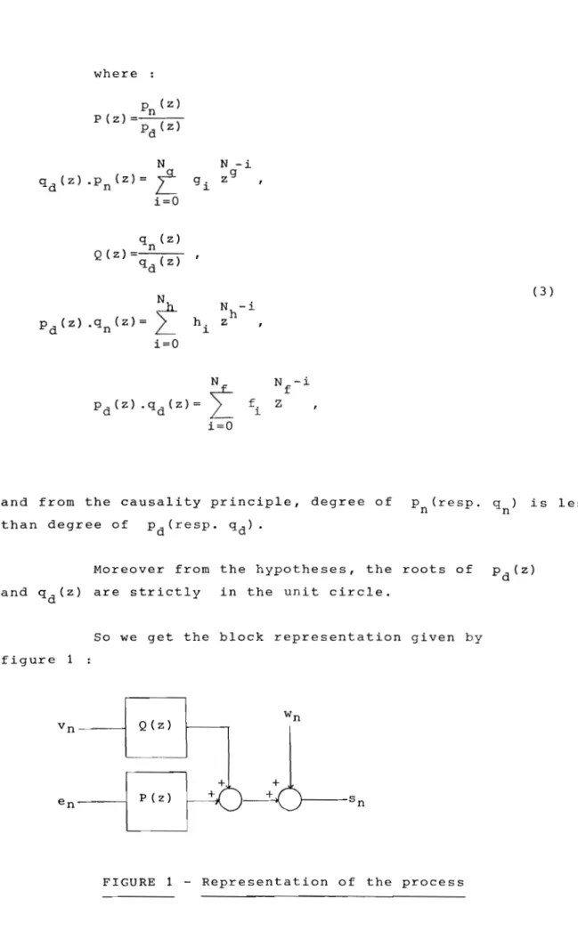
A-2.1.3 Representation of the mathematical model of the process

With hypotheses Hl, H2, we compute the output s(n), from the inputs e(n) ,v(n) ,w(n) by the recursive equation :

N

e n - i + L h i v n_ i

฀฀฀

(1)

time invariant scalars.

Neglecting the i n i t i a l conditions (justified by asymptotic stability), we can represent (1)

a more concise way using z - transforms

s(Z)=P(z)e(z)+Q(Z)v(Z)+w(Z) (2)

A-2.1. 2.2 Hypothesis on disturbances (E2) ,

We suppose both measured and unmeasured disturbances to be causal and to admit z - transforms which verify conditions of final value therorem

[lJ.

I f the disturhances are represented as stochastic processes, these hypotheses are made on the

mathematical expectationsand aIl the following deterministic results must he considered in mathematical expectation.

Moreover we suppose the output to be lineraly time-invariant dependant on the disturbanees. SO we introduce a new linear, time invariant, asymptotieally stable operator Q between the measured disturbance and the output.

A-2. 1. 3 ฀฀฀฀฀฀฀฀฀฀฀฀of the mathematieal model of the proeess

With hypotheses Hl, H2, we compute the output s(n), from the inputs e(n) ,ven) ,w(n) by the recursive equation :

N

N

f i _{Sn_i=f gi e n _i}

+

L

hi v n _i

i"'O i=O

are time invariant scalars.

Neglecting the i n i t i a l conditions (justified by asymptotic stability) , we can represent (Il in a more concise way using z - transforms

s [z) =p (z) e (z) +Q (z) V (z) +w (z)

(1)

p (z) p ( z ) = _ n _ Pd (z) N N - i qd (z) .Pn(z) =

L

gi zg , i=O qn (z) ฀฀฀฀฀฀฀ (3) N P d (z) ·qd (z)=

t

i=O N - i f f i Z

and from the causality principle, degree of P

n ( r e s p . qn) i s less than degree of P

d (resp. qd).

Moreover from the hypotheses, and qd (z) are s t r i c t l y in the unit circle.

roots of P d (z)

So we get the block representation given by figure 1

FIGURE 1 - Representation of the process

฀฀฀฀฀฀฀

_{Pd (z)} N N - i

฀฀฀฀฀฀฀฀฀฀฀฀฀฀

gi zg i=O N Pd {zl ·qd (zl =

t

i=O

(3)

and from the causa l i t y principle, degree of Pn (resp. qn) is less than degree of Pd (resp. qd)·

Moreover from the hypotheses, the roots of Pd (z) and qd{z) are s t r i c t l y in the unit circle.

50 we get the black representation given by figure 1

A-2.2 Definition of a set of specifications

A-2. 2.1 ฀฀฀ regulation

We want the effect of non decreasing distur-on the process to be, in some sense, minimized or

Given an external non diminishing signal set point and noted un ' we want the output n to track un with minimal or ideally, zero steady state error. For this problem, we impose a causal set point with z - transform which verifies conditions of the

A-2.2.3 Internal stability

In both cases i t is also imperative that an appropriate control law be designed in such a way as to insure an asymptotically stable design i . e. the relations between the external signals (set point, measured and

unmeasured inputs) and the internal signals (control, output) must be stable in some sense.

A-2. 2. 4 ฀฀฀฀฀฀฀ convergence

We will summarize the preceding definitions by the asymptotic convergence of the output sn

set point un

(4)

A - 2 . 2 _{Definition of a set of specifications}

A - 2 . _{2.1 Output regulation}

We want the effect of non decreasing distur-bances on the process to be, in some sense, minimized or eliminated.

Given an external non diminishing signal called the set point and noted un ' we want the output Sn to track un wi th minimal or ideally, zero steady state error. For this problem, we impose a causal set point with z - transform which verifies conditions of the final

A - 2 . 2 . 3 _{InternaI stability}

In both cases i t is also imperative that an appropriate control law be designed in such a way as to insure an asymptotically stable design

i . e .

the relations between the external signaIs {set point, measured and

unmeasured inputs) and the internaI signals {control,output) must be stable in sorne sense.

A-2. 2. 4 ฀฀฀฀฀฀฀฀convergence

We will summarize the preceding definitions by the asymptotic convergence of the output sn

set point un

In fact we have only here the least constraints to set any system of control. The synthesis of such a system must also take into account the behaviour of this convergence and need performance criteria

[21.

From greater variability we keep ourselves wi thin the convergence cr i t e r ion.

A-2.3 Definition of the control law

We call control law a method to compute future

given the observation of a l l the measurable past signals. To get a very general linear time-invariant control, we compute a future control e

n+ 1 ,given the past measured signals

(em' sm' urn' v_m ; m ฀ n) as a finite linear combination

N e(n+l)

=-r

i=O sn_i+

t

_{r i u n_ i-}

t

i=O i=O (5) Or using z - transforms, we wr i te : c (z) e (z) =r ( z ) u (z) -d (z) S (z) -b (z) v (z) (6)

c(z), r(z), d(z), b(z) z - polynomials such that degree of c(z) is greater than degree of r(z), d(z) or b(z) and c(z) is mutually prime with r(z), d(z) and b(z).

Note that from the homogeneity of equation (6),

is no use to take rational functions instead of polynomials.

A-2.3.2 Interpretation

Equation (6) has the block diagram representation given figure 2.

In fact we have only here the least constraints ta set any system of control. The synthesis of such a system must also take into account the hehaviour of this convergence and need performance criteria [2]. From greater variability we keep ourselves within the convergence criterion.

A-2.3 Definition of the control law

A-2.3.l Definition

We calI control law a method ta compute future con troIs given the observation of aIl the measurahle past signaIs. Ta get a very general linear time-invariant control, we compute a future control _{e n}

+

₁ ,given the past measured signaIs

N

e(n+l)=-r i=O

m ฀฀nl as a finite linear combination

Or using z - transforms, we write

c (zl e (z) =r (z) u (zl-d (z) s (z) -b (zl v (zl

with c(z), r(zl, d(zl, b(z) z - polynomials such that (5)

(6)

degree of c(z) is greater than degree of r(z), d(z) or b{z) and c(z) i s mutually prime with r(z), d(z) and b(zl.

Note that from the homogeneity of equation ( 6 ) .

is no use to take rational functions instead of polynomials.

Equation (6) has the black diagram representation given figure 2.

FIGURE 2 - Control law structure

So we can interpret the four parameters c,r,d,b of the control law as [3] :

c (z) a compensator

d (z)

r (z) is a reference

b (z) is a feed_forward input

FIGURE 2 - Control law structure

So we can interpret the four parameters c,r,d,b of the control law as [3] ,

c (z) is a compensator

d (z) is a sensor

r (z) is a reference

A-3 Relations between parameters of the control

A-3.1 study of the closed loop-system

We study the closed loop-system in i t s asymptotic behaviour. So we are going to express the various

between external and internal signals :

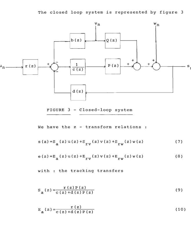
The closed loop system is represented by figure 3

FIGURE 3 - Closed-loop system

s (z) =Sa (z)U (z) +Srv ( a ) v (z) +Srw (z) w (z )

e (z) =E

a (z) u (z) +Er v (z) v (z) +Er w(z) w ( z ) with : the tracking transfers

E_{a (z)} c (z)

฀฀ ฀฀฀

p (z)

(7)

(8)

(9)

(10)

A-3 Relations between parameter5 of the contTol

A - 3 • 1 S t u ฀฀฀฀฀฀฀฀฀฀฀฀฀฀฀h",",-"=,,,"-",' ฀฀฀฀฀฀฀฀฀"'C Y"'"Cot e"",m

behaviour.

Wc study the

going ta

loop-systcm in i t s asymptotic the various transfers between extern"l and internal signals

The closed loop system i s represented by figure 3

FIGURE 3 - Closed-laop system

We have the z - transform r\'?lations

s (z) "'Sa (z) u (z) +Srv(z) v (z) +Srw (z) wez)

(7)

e (2) =Ea (z) U (z) +Erv (z) V (z) +Erw (z) W (z) (8)

the tracking transfers

(9)

10

and the regulation feedback and feed forward transfers

c (z) c (z) +d (z)P (z) b (z) +d (z) Q (z) c (z) +d (z) P (z) d (z) c (z) +d(z) P (z) (11) (12) (13) (14)

We can see that the poles of any transfer are given by the roots of the expression c(z)+d(z)P(z). Moreover from the s t a b i l i t y of P(z), Q(z) and the hypothesis of

mutual primeness, a necessary and sufficient condition of internal s t a b i l i t y is given by the s t a b i l i t y of the control and more precisely by the s t a b i l i t y of the E

a (z) transfer.

We shall note that given the s t a b i l i t y conditions, sensor d(z) determine the Erw(Z) regulation transfer, the compensator c (z) determines the Sr

w(z) regulation transfer and r(z) determines the Ea(Z) tracking transfer. With

tracking transfer :

remark that the difference between d(z) and r(z) differenciates between regulation and tracking behaviours.

whi th expression (11), i f i t i s possible to get

c (z) Q(z) =b (z) P (z) (16)

we will be able to compensate completely the measured

distur-10

regulation feedback and feedforward transfers

E (zl=_b(z)+d(zlQ(z) rv c(z)+d(z)P(z) E (z)=o- d(z) rw c(z)+d(z)P(z) (11 ) (12) (13) ( 14)

l'le can see that the poles of any transfer are given by the roots of the expression c(z)+d(z)P(z). Moreover

stability of P (z), Q (z) and the hypothesis of mutual primeness, a necessary and suffi aient condition of internaI stability ls given by the s t a b i l i t y of the control and more precise!y by the stability of the Ea (z) transfer.

We shall note that given the stability conditions, sensor d(z) determine the Erw(z) regulation transfer, the compensator c(z) determines the Srw(z) regulation transfer and r(z) determines the Ea(Z) tracking transfer. With

tracking transfer ,

1 _ 5 (z)=5 (z)+(d(zl-r(z»P(z)

a

rw c(z)+d(z)P(z)

we remark that the difference between d(z) and r(z) differenciates between regulation and tracking behaviours.

( 15)

Whith expression (11), i f i t i s possible to get

c(z)Q(z)=b(z)P(z) (16)

distur-From expressions (9), (11), (12), we expression (4) using the final value theorem

lim (l-z) ( s (z) -u (z»;O

Supposing s(z) ,u(z) to be defined in the ring

(1, + CO ) . separate set-point, measured and

unmeasured disturbances actions, we will transpose specifications into four constraints

regulation constraints :

tracking constraint :

And stability constraint

The roots of c(z) Pd(z)+d(z)Pn(z) are s t r i c t l y in the unit cercle.

A-3.2 Regulation constraints

Passive regulation

We want to impose relation (18). with the hypothesis on the process and if- the sensor has a non

static gain, i t is necessary and sufficient that :

(17) (18) ( 19) (20) c (1) =0 (21) 11

From expressions (9) 1 (11). (12), we can write

expression (4) using the final value theorem

lim (1-z) ( 5 (z)-u(z»=o

Supposing s(z) ,u(z) ta be defined in the ring (1,+ 00 ). In arder ta separate set-point, measured and unmeasured disturhances actions, we will transpose the

specifications into four constraints

regulation constraints :

tracking constraint :

And stability constraint

The roots of c(z) Pd(z)+d(zlPn(z) are s t r i c t l y in the unit cercle.

A-3.2 Regulation constraints

A-3. 2.1 ฀฀฀฀฀฀฀฀฀฀฀฀฀฀฀฀

We want ta impose relation (18). With the hypothesis on the process and i f ' the sensor has a non

static gain, i t 15 necessary and sufficient that

c (1) =0 (17) (18) (19) (20) (21)

12

So, we must impose a factorization of the compensator in

c (z)

=

(z-l) m (z)

Moreover, from now on, we will write the k d(z) with

d (1) =1, k;<O

From the preceding resul t s , impose

b (1) =0

So, we have the following factorization

b (z)

=

(z-l) n (z)

A-3.3 Tracking constraint

(22)

(23)

(24)

(25).

We verify expression (20) i f we impose identical s t a t i c gains for both sensor and reference. So as in (23), from now on, we will write the reference as k r (z)

r (1) =1, kT"O

A-3.4 Remark

(26)

With expressions (22), (23), (25) and (26), (6) must

zm(z)e(z)=m(z)e(z)+(z-l)n(z)v(z) +k(r(z)u(z)-d(z)s(z» (27)

12

Sa, we must impose a factorization of the compensator in

c(z)=(,,:-l)m(z) (22)

Moreover, from now on, we ฀฀฀฀฀write the

k d(z) w i t h ,

(23)

A-3.2.2 Active requlation

From the preceding results, impose :

b(1)=O (24)

Sa, we have the f0110wing factorization

b{z}=(z-l)n(z) (25).

A-3.3 Tracking constraint

Ws verify expression (20) i f we impose identical

static gains for bath sensar and referenes. So as in (23), from now on, we will write the referenee as k rIz) with :

r(1)=1, k .... O (26)

A-3.4 Remark

With expressions (22), (23), (25) and (26), (6) must

So the control is computed in a recursive way.

A-3.5 Stability constraint

We study the polynomial

(z-l)m(z)Pd(z)+kd(Z)Pn(z)

We know already :

- Pd (z) has a l l i t s roots s t r i c t l y in the unit circle - k,d(l),Pn(l) are different from zero

- degree of m (z) is greater than degree of d (z)

- degree of Pd (z) is greater than degree of Pn (z)

wi th no more hypothesis on the process, we can give a sufficient condi tion of internal stability (Proof in Appendix 1).

If m(z) has a l l _{i t s roots s t r i c t l y in the unit}

circle, i t exists a vicinity of zero v

t

o) such that i f k is in V(a)-(O), internal asymptotic stability is ensured

and only i f :

km(l)P(l»

a

(stability condition)

P (1) equal to the static gain of the process.

(28)

Note that from continuity, the existence of a vicinity can be transposed on the existence of a vicinity of p (z) as we will see in a next section, and so this permits the study of robustness as i t was formulated in the

introduc-13

So the control 15 computed in a recursive way.

A-J.5 Stabili ty constraint

liIe study the polynomial

(z-1) ID (z) Pd (z) +kd {z} Pn (z)

\ile know already :

Pd (z) has aIL i t s roots s t r i c t l y in the unit circle

- k,d{1} ,Pn (1) are different from zero

- degree of m(z) 16 greater than degree of d(z)

- degree of Pd(z) 19 greater than degree of Pn{z)

with no more hypothesis on the proci'!ss, we can give a su i f i c i e n t condition of internaI s t a b i l i t y (Proof in Appendix 1).

I f wez) has aIL l t s r-DotS s t r i c t l y in the unit circle, l t exists a vicinity of zero V(O) such that i f k is in V{O)-(Q), internaI asymptotic s t a b i l i t y 15 ensured

i f and only i f ;

km(1)P(11> 0 (stability condition) (28)

with pel) equal ta the static gain of the proces5.

Note that from continuity, the existence of a vicinity of k can be transposed on the existence of a vicinity of P (z) as we will see in a next section, and so this permits the study of robustness as i t was formulated in the

introduc-A-3.6 Introduction of a non linearity on the control

We will extend here the results of Rouhani

[4J.

introduce a non linear compensator defined as follows

(figure 4).

y n be the input signal of the compensator, compute the control en through the expression :

N-l e_{n+ 1}=f_n

(n%-

(y n +

L

(m_i-w_i +₁₎ e_{n_ i} +mNe _{n_ N} » i=O W(Z)=f m i zN-i i=O f

n (x) a real time varying function

FIGURE 4 - Non linear compensator

(29)

To study the behaviour of the closed-loop system, we give an asymptotic value

u

to the set point, we compute a theoretic asymptotic value

e

of the control :

p(l)e=u (30)

suppose the disturbances ฀฀฀be bounded and the processes to be a M.A. system (P(z)=z P Pn(z)),

A-3.6 Introduction of a non linearity on the control

We will extend here the results of Rouhani

[41.

introduce a non linear compensator defined as follows

(figure 4).

y n be the input signal of the compensatar, compute the control en through the expression

N-1

฀฀฀฀฀฀฀฀฀฀฀

(Yn+L (mi-mi+l)en_i+mNen_N

»

i"'O

with m(z)'"

f

mi zN-i

i"'O

f _n (x) a real time varying function

y

฀

n

฀฀฀฀

e

n (z-l)m(z) n+1

FIGURE 4 - Non linear campensator

'1'0 study the behaviour of the closed-Iaap system, give an asymptotic value

u

ta the set point, we compute a theoretic asymptotic value

e

of the control

(29)

p(l)e"'u (30)

We suppose the disturbances ฀฀฀฀be bounded and the processes to be a M.A. system (p (z) =Z P Po ( z » .

Then we can say (Proof in Appendix 2) :

Let./ be the greatest modulus of the roots of

(z-1)m(z)z P+kd(z)Pn(z), i f for any n we have for a certain

X N_{p - 1}

f

n (xNp

+e)-e

<

฀

y

, k <.1 (31)

then the non linear system i s

In fact here (with the hypothesis on the disturbances) s t a b i l i t y i s taken in the sense of bounded input bounded output (bibo). But i f the external signals (set-point,

disturbances) become constant, i t will become an asymptotic s t a b i l i t y and verify relation (4).

Then we can say (Proof in Appendix 2) ,

Let? be the greatest modulus of the roots of

(z-l)m(z)zNp+kd(Z)Pn(Z), i f for any n we have for a certain

X

o

X

o

<

k

k ( l

(31)

XN p _l

r

XN_p- l f n (xNp

+e)-e

XN_p

non linear system i8

In fact here (with the hypothesis on the disturbances) stabili ty is taken in the sense of bounded input bounded output (bibo). But i f the external signals (set-point,

disturbances) become constant, i t will become an asymptotic stability and verify relation (4).

Sensitivity of the convergence criterion

Following our introduction we are going to study the sensitivity of our preceding results to variations of P and Q. In fact given the parameters m,r,k,d,m of the control law, we are looking for the set of P,Q operators for which the convergence criterion is satisfied. To keep the validity of our approach, we will take P,Q in the class of linear time invariant processes.

At once l e t us remark that only the stability constraint uses hypothesis on P and Q, so we can conclude to

insensitivity of the tracking and regulation constraints. And from now on we will look at the stability problem.

From expressions (9) to (14) i t is easy to conclude that for any asymptotically stable Q, we will

stability. So, in fact, there is no sensitivity to

Q.

A-4.2 Sensitivity to P

In the hypothesis HI we have imposed P additional constraints to those on Q, particularly rational type and non zero st a t i c gain. The l a t t e r was essential in regulation

and stability constraints. So we must impose variations of P to maintain the sign of the static gain. The former was a theoretic facility but i t can be relaxed.

A-4. 2.1 P of rational type

In that case we have to find a l l the pairs of polynomials (Pn (z), Pd Cz ) such that :

A-4 Sensitivity of the convergence criterion

Following our introduction we are going to study the sensitivity of our preceding results to variations of P and Q. In fact given the parameters m,r,k,d,m of the control law, we are looking for the set of P,Q operatorE for which the convergence criterion is satisfied. To keep the validity of our approach, we will take P,Q in the class of 11near time invariant pro cesses .

At once l e t us remark that only the stability constraint uses hypothesis on P and Q, 50 we can conclude to

insensitivity of the tracking and regulation constraints. And from now on IVe will look at the stability problern.

A-4.1 Sensitivity to Q

From expressions (9) te (14) i t is easy te conclude that for any asymptotically stable Q, we will internaI stability. so, in fact, there is no sensitivity to Q.

A-4.2 Sensitivity to P

In the hypothesis Hl we have imposed P additional constraints ta those on Q, particularly rational type and non zero static gain. The latter was eEsential in regulation

and Etability constraints. SA we must impoEe variationE of p te main tain the sLgn of the static gain. The former was a theoretic facility but i t can be relaxed.

A-4. 2.1 P of rational type

In that case we have to find aIl the paLrs of polynomials (Pn (z), Pd (z» Euch that

degree of P

d is greater than degree of Pn' and the roots of Pd(z) and (z-l)m(z)Pd(z)+kPn(z)d(z) are s t r i c t l y in the unit circle.

Pd (z) and the number (N

p+l) of coefficients of Pn(z), suppose m(z) has a l l i t s roots in the unit c i r c l e , we look for the coefficients _{PO, . . • . . ,PN p such that the}

polynomial

฀ N - i

฀฀฀฀฀฀฀฀฀฀฀฀฀฀฀฀฀฀฀฀฀฀฀฀฀

L

Pi z P (32)

฀฀฀

has a l l

Let us work in the g (z) coefficients

be a vector representative of g (z) ,

M

be representative of (z-l)m(z)P d(z),

P

be representative of P

n (z) ,

D be a matrix representative of the of d(z) on p(z).

(33)

G i s linearly dependant on

P.

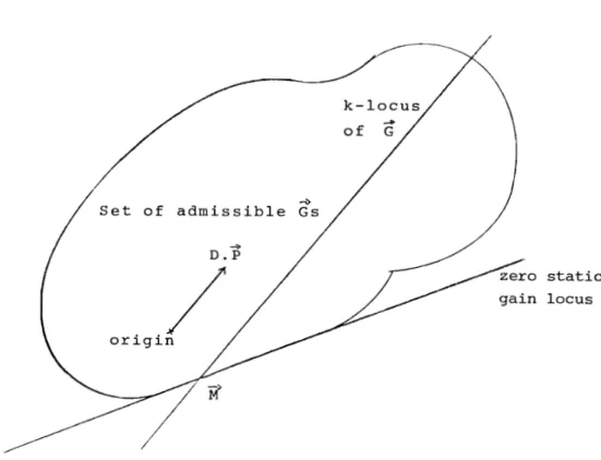
Otherwise, given the highest degree coefficient of m(z) Pd (z), from the continuity of the coefficients on the roots, we can say that the set of admissible Gs which represent polynomials whose roots are in the unit c i rc l e i s closed, bounded and connected. Moreover from the presence of (z-l), we can say that

M

i s on the frontier of t hi s

Thus we have the situation given by figure 5.

17

degree of Pd 15 greater than degree of Pn' and the roots of Pd(z) and (z-l)m(zlPdCzl+kPn(zld(z) are s t r i c t l y in the unit circie.

Pd(zl and the number CNp+l1 of coefficients of Pn (1'.), suppose m(z) has aIl i t s roots in the unit cirele, we look for the coefficients PO" _ •.. ,PNp such that the

polynomial

g(z)""(z-l)m(zlPd(z)+kdCz)

฀฀

Pi zNp-i (32)

฀฀฀฀

has aIl i ts roots in the unit cirale.

Let us work in the g(z) coefficients space.

be a vector representative of 9 (z) , representative of (z-l)m(zlPd(z),

representative of Pn (1'.),

D be a matrix representative of the

of d(z) on pCz).

G=M+kD.P,

G ls linearly dependant on P.

(33 )

Otherwise, given the highest degree coefficient of m(z) Pd (z), from the continuity of the coefficients on the roots, we can say that the set of admissible Gs which represent polynomials whose roots are in the unit circle is closed, bounded and connected. Moreover from the presence of (z-l) 1 we can say that

M

is on the frontier of this

of

G

Set of admissible Gs

D.P

gain locus

FIGURE 5 - Coefficient representation of stability constraint

So from the knowledge of the set of admissible Gs, we can find the set of admissible Ps. The f i r s t set has been studied by Markov [6J in the continuous case. Particu-larly we can' t make sure of convexity of the set, so

the linearity we don' t know i f the set of admissible

PS

i s connected.

This approach gives the roles of In, d or k : m corresponds to a translation, d is very similar to a rotation and k to a linear displacement. Moreover we see the coupling between vicini ties of k and P.

18

Set of admissible GS

gain locus

FIGURE 5 - Coefficient representation of st a b i l i ty

constraint

So from the knowledge of the set of admissible Gs, we can find the set of admissible Ps. The f i r s t set has been studied by Markov [6] in the continuous case. Parti

cu-larly we can' t _{wake sure of convexi ty of the set, 50}

the linearity we don't know i f the set of admissible Ps 18

connected.

This approach gives the roles of m, d or k : ID corresponds ta a translation, d ls very similar ta a

rotation and k te a 11near displacement. ฀฀฀฀฀฀฀฀฀฀we can

19

A- 4 . 2 . 2 P i n the vic i nit y 0 f a r at ion a l P

0-Suppose the parameters of the control

f i t t e d to a nominal process Po of rational type. We are looking for variations /':,. P around PO' such that we

internal stability.

If we suppose P (z) to be an analytic function a domain s t r i c t l y contained in the unit circle and

9 ( z) = (z -1 )m ( z ) + kd ( z) Po (z)

h (z) =kd (z) l:,.P (z)

Then g

(±)

and h

(±)

are analytic in and on the uni t circle and with the

Ro

u c h e Theorem

[7]

,

we can

for any process P(z)=PO(z)+Ap(z) such that

(34)

(35)

sf [- n, n)

(36)

we will have internal stability.

We have in fact here another presentation of resul t of Doyle

[8)

in the SI SO case.

A-4.2.3 Application to a polynomial variation

Let us take 6.P (z) of the form :

N 6 P ( Z ) = [ lIPjzM- j j=O Expression (36) means : (37) I(eil> -1) m (ei G) +kd (ei 9)Po (ei

6' )1

>

k Id (ei 9)

Ilh.p

(ei 8) /.(3 8 ) V9 E:

[_n,

11J

19

A-4.2.2 P in the vicinity of a rational

PO-Suppose the parameters of the control law ta f i t t e d te a nominal process Po of rational type. We

are looking for variations

.6.

P around PO' such that WB

have internal stabi1.ity.

I f WB suppose P (l'Il ta be an analytic function outside a domain s t r i c t l y contained in the unit circie and

i f WB note

9 (l'Il'" (z-1) m (z) +kd (z)

Po

(l'Il

h(z)=kd(z)h..P(z)

Then 9

฀฀฀฀

and h

(±J

are analytic in and on

unit cirela and with the Rouché Theorem [7} • WB can say for any process P (1':) =P_o (l'Il +/lP (z) such that

sE: [- n, n]

WB will have internal stability.

We have in fact here another presentation of result of Doyle [8) in the SISO case.

A-4.2.3 Application ta Cl. polynomial variation

Let us take ll.P (zl of the form :

6.P (z)

=:["

e.PjzM-j j=O Expression (36) (34) (35) (36) (37)

฀฀฀฀฀฀

-1) m (e11<) +kd (e 19 ) Po (ei 5')1

>

k Id (ei @)IJll.P(e 10 )jpS)

VB

é.

[_11,

nJ

But we have wi th appendix 3 :

IAP(ei 9

) 1

2=

i

APj API cos(j_l)$ (39)

j ,1=0

2 N

฀฀฀฀฀฀฀฀฀

«L

฀฀฀฀฀฀฀฀฀฀฀฀฀฀฀฀฀฀฀฀฀

I)

(40) j=O

c.a n get an upper bound of the modulus 1

(f

฀฀฀฀฀

<

min l(ei':l)m(e i e )+kd(eiS)Po(eil9\ j=O

rN.[-n

฀฀฀฀฀฀฀฀฀฀฀฀฀฀฀฀฀฀฀฀฀฀฀฀฀฀฀฀฀฀฀฀฀฀

(41)

Practically an FFT algorithm will provide spectra.

A-4.2.4 Convergence criterion sensi tivi ty index (CCl)

Given a process Po and the parameters of control law we define an absolute index by :

From expression (36) this index gives an upper bound on the possible spectrum variation to verify convergence criterion. So we call i t a convergence criterion sensitivity index. To insure robustness, i t has to be compared with an equivalent approximation index given by the Po model estimation phase.

20

But we have with eppendix 3 :

IAP(eiG

)1

2=

t

6.Pj API cos(j_l}e j ,1=0

(39)

2 N

IAP(e!!})1

«L

฀฀฀฀฀฀฀฀฀฀฀฀฀฀฀฀฀฀฀฀฀฀

(40)

j=O

a,an get an upper bound of the modulus

1

,f

2

'<

min

฀฀฀฀฀฀฀฀฀฀฀฀฀฀฀฀฀฀฀฀฀฀฀฀฀฀฀฀฀฀฀

AP j )

'h

j=O BE [-11 ,+11] k

Id

(e19 )

฀฀฀฀฀฀฀฀฀฀฀฀฀฀฀฀฀

11

2

Practically an FFT aigori thm will provide these spectra.

A-4. 2.4 Convergence cri terion sensitivi

ty

index (CCI)

Given a proc€ss Po and the parameters of control law we define an absolute index by :

the

(41 )

(42)

From expression (36) this index gives an upper bound on the possible spectrum variation ta verify convergence criterion. SA we calI i t a convergence criterion sensitivity index. Ta in sure robustness, i t has ta be compared with an equivalent approximation index given by the

Po

model estimation phase.

21

In this f i r s t part, we came back on the problem of linear control. The most important results have been

reformulated in a very general way: resul ts on the structure of the control law, results on stability in the linear case and in a simple non linear case and at l a s t results on a measure of the sensitivity of st a bi l i t y.

2!

A-S sUIlIJIlary

In th!s f i r s t part, we came back on the problem of

linear control. The mest important results have been

reformulated in a very general way : results on the stI"ucture

of the control law, results on stability in the linear case

and in a simple non linear case and at l a s t results on a

B. THE SINGLE INPUT-SINGLE OUTPUT (SISO) ADAPTED MODEL ALGORITHM CONTROL (AMAC)

We have just presented a linear time invariant control law in a general fashion. It is an abstract approach which serves only to ensure the convergence criterion. In an attempt to get behavior criteria, we are going to give a physical presentation through a SISO control based on the mathematical representation of the process of paragraph A-2.l.3:

s(z) ฀ P(z)e(z)

+

Q(z)v(z)

+

w(z)

and the use of adapted models of the operators P,Q.

B-l. General SISO AMAC Presentation B-l.l Definition of the Strategy

(1)

At time n , given the past measurable signals, the S1S0 AMAC computes a control such that a predicted output of the process is identical to a predicted set point.

Taking the notation of Box and Jenkins [9], we write this:

the prediction being here of one point ahead. From the representation of the process (1) we decompose the predicted output into two parts: a deterministic part which functionally depends on the inputs and a non-deterministic part sUn(l) resulting from the disturbances. Let M(en(l), e£: £':<:=n) be a model of the operator P which defines the deterministic

B. THE SINGLE INPUT-SINGLE OUTPur (SISO) ADAPTED MODEL ALGORITHM CONTROL (AMAC)

We have just presented a linear time invariant control law in a

general fashion. It i8 an abstract approach which serves oniy ta ensure

the convergence criterion. In an attempt ta get behavior criteria, we are

going to give a physical presentation through a SISO control based on

the mathematical representation of the process of paragraph A-2.1.3:

S(z) ฀฀p(z)e(z)

+

Q(z)v(z)

+

wez) (1)

and the use of adapted rnodels of the operators P,Q.

B-l. General SISO AMAC Presentation

B-1.1 Definition of the Strategy

At time n. given the past measurable signais, the SISO AMAC computes

a control such that a predicted output of the process is identical ta a

predicted set point.

Taking the notation of Box and Jenkins

[9J,

we write this:

the prediction being here of one point ahead. From the representation

of the proceSB (1) we decompose the predicted output into two parts: a

deterministic part which functionally depends on the inputs and a

non-deterministic part sun(l) resulting fram the disturbances. Let M(en(l),

23

output from the future and past controls, we deduce from (2) the control law as:

(3)

Then to compute the control en (1) we have three different problems: inversion of M, estimation and prediction of the non-deterministic out-put, and prediction of the set point.

From its definition, M is a model of the process. Note that to

compute en (1), we use this model in a reversed way compared to the physical transfer, sa we require M to be invertible in the sense defined by Box and Jenkins [9] and we call i t a deconvolution model. Thus with the linear time invariant hypothesis the model of the process is taken linear, time invariant, asymptotically stable, of rational type and invertible.

Let rod

i or Md(z) be the impulse response and the rational z-transform of this deconvolution model. We obtain from (3)

(4)

and md

O must be different from zero.

B-1.3 Estimation and Prediction of the Non-Deterministic Output From expression (1) the non-deterministic output is the sum of both a filtered measured disturbance v

n and an unmeasured disturbance wn. Suppose we have an estimation

w

_n of w

n and a convolution model of the

23

output from the future and past con troIs • Iole deduce from (2) the <'-ontrol lawas:

(3)

Then ta compute the control e n (l) Iole have three different problems:

inversion of M. estimation and prediction of the ฀฀฀฀฀฀฀฀฀฀฀฀฀฀฀฀฀฀ out-put, and prediction of the set point.

B-l.2 Inversion of the Model M

From its def!nition, M 18 a mode! of the process. Note that: te

compute en (1). Iole use this model in a reversed way compared te the physical

transier, se Iole require M to be invertible in the sense defined by Box and Jenkins [9] and we calI i t a deconvolution rnodel. Thus 'Io7ith the

linesr time invariant hypothesis the model of the pro cess 18 taken linesr.

time invariant, ssymptotically stable, of rational type and invertible.

Let md! or Md(z) be the impulse response and the rational z-transform

of this deeonvolution model. We obtain from (3)

(4)

and

md

_{O must be different from zero,}

B-l.3 Estimation and Predietion of the Non-Deterministie Output

From expression (1) the non-detenninistic output is the SUlll of both

a filtered measured disturbance v n and an unmeasured disturbance w_{n '} Suppose we have an estimation On of IOn and a eonvolution model of the

measured disturbance filter Q : nC

i (Nc(z», then if vn(1) and

w

n(1) are predictions of measured and unmeasured disturbances, we compute:

(5)

So we first need the estimation w

n(1) of the unmeasured disturbance and secondly measured and unmeasured disturbance predictors.

We already introduced a convolution model Nc of Q. Let us take also a new model mC

i(Mc(z» of the process P. This time we need a model to be used in the same way as the process so Mc(z) is a convolution model com-pared with Md(z), a deconvolution model. Similarly to expression (1), we compute the estimation

w

n by

00 00

w

n = sn - iI

_o

mCi'en_ i - iI

_o

nCi'vn_ i

Now from the past v

n and

w

n' we want to predict 3un(1). From discrete parameter prediction theory [10], vn(l) and wn(l) can be computed with prediction filters. Using a-rtr ansf o rms they may be expressed as

vel) (z)

=

Fv(Z) v(z)

=

฀฀฀฀฀฀

v(z)

(7)

where fwn(z), fwd(z), fvn(z), fvd(z) are polynomials in z , the degree of fwd(resp fvd) being greater than the degree of fwn(resp fvn). Moreover, to be able to predict the continuous component of the disturbances, we

measured disturbance fil ter Q : nei(Nc(z», then if vn(l) and wn(l) are

predictions of measured and unmeasured disturbances, we compute:

(5)

So we first need the estimation wn (1) of the unmeasured disturbance and secondly measured and unmeasured disturbance predictors.

We already introduced a convolution model Ne of Q. Let us take also

a new model mci(Mc(Z» of the process P. This time we need a model to be

llsed in the same way as the proeess so Mc(z) is a convolution model

com-pared with Md(z), a deconvolution model. Similarly ta expression (1), Ioire

compute the estimation Wn by

.

.

On - sn - iIo mci"en _i -

ilo

nCi"Vn_ i

Now from the past v n and wn ' we want to predict ฀฀฀(1). From dis crete parameter prediction theory [10], vn(l) and wn(l) can be computed with

prediction filters. Using lI-transforms they may be expressed as

vell (z) = Fv(z) vez) '"

฀฀฀฀฀฀฀

vez)

(7)

",here fwn(z), fwd(z), fvn(z), fvd(z) are polynomials in z, the degree of

fwd(resp fvd) being greater than the degree of fwn(resp fvn). Moreover,

impose unit static gain predictors.

Thus we get the z-transform of BUn (1) :

su(l) (z) = Nc(z) v(z)

+

Fw(z) w(z)

with Nc' (z) ฀฀฀฀฀ computed from N

c and Fv through the relation:

00 00

ncO v n (1)

+

฀฀฀

nC i v n

+

l -i =

฀฀฀ ฀฀฀

_{v n_ i}

Now from z-transform of (6) we have the final relation:

(8)

(9)

su(l)(z) = FW(z) (s(z) -Mc(z)e(z))

+

฀฀฀฀฀฀ -Fw(z)Nc(z))v(z) (10)

or equivalently in the time domain:

where

*

represents the discrete convolution operator.

B-1.3 Set Point Prediction

(ll)

To get a better behavior of the closed-loop system, at time n we need future set points. In some cases they are available (particularly when there is a hierarchical control). But generally we need a predictor. Let us take i t in the form of a rational filter Fu(z) with fU

i as impulse response and with unit static gain.

u(l)(z)

=

Fu(z)u(z)

=

฀฀฀฀฀฀

u(z) (12)

impose unit static gain predietors.

Thus we get the z-transfonn of sUn (1):

suCl) (z) ฀฀NeCz) vez)

+

Fw(z) f./(z) (8)

with Ne'(z) (nei) computed from Ne and Fv through the relation:

.

.

ne a vn(l)

+

฀฀฀฀

ne i v n

+

l _i =

฀฀฀฀

_{nei v n _i} (9)

Now from z-transform of (6) we have the final relation:

8u(1)(z) - Fw(z)(s(z) -Me(z)e(z»

+

฀฀฀฀฀฀฀- Fw(z)Ne(z»v(z) (10)

or equivalently in the time domain:

(11)

where il: represents the discrete convolution operator.

B-1.3 Set Point Prediction

To get a better behavior of the closed-loop system, at time n we

need future set points. In 60me cases tbey are available (particularly

when there i8 a hierarchical control). But generally we need a predietor.

Let us take

i t

_{in the form of a rational fil ter Fu(z) with fUi as impulse}

response and with unit statie gain.

(13)

with fun(z), fud(z) polynomials in z, with the degree of fud(z) greater than or equal to the degree of fun(z).

B-1.4 Expression and Properties of the 5150 AMAC Law

From expressions (3), (11) and (13) we get the 5150 AMAC law

(14)

This prediction is used as the future control e

n

+

l. Thus we get the z-transform representation of the 5150 AMAC law:

(zoMd(z) - Fw(z) oMc(z»e(z) = Fu(z) ou(z) - Fw(z)s(z)

- (Nc' (z) - Fw(z)Nc(z) )v(z) (15)

Then we find the expression of the four polynomials of our general linear time invariant control law:

c(z) = zoMd(z) - Fw(z)Mc(z) r(z) = Fu(z)

(16) d(z) = Fw(z)

b(z) = Nc' (z) - Fw(z)Nc(z)

Thus we can give a physical interpretation to these polynomials. Moreover, we see that from a physical point of view c, r , d and b are not mutually independent, but Md or Mc, Nc , Fu , Fv and Fw are.

(13)

with ฀฀฀฀฀฀฀฀ ฀฀฀฀฀฀฀po1ynomia1s in

z,

with the degree of fud(z) greater than Or equal to the degree of ฀฀฀฀฀฀฀฀

B-l. 4 Expression and Properties of the S150 !MAC Law

From expressions (3), (11) and (13) we get the S150 !MAC 1aw

This prediction is used as the future control e_n

+

_{1 •} Thus we get the z-transfonn representation of the SISO !MAC law:

(z'Md(z) - Fw(z) 'Mc(z»e(z) = Fu(z) 'u(z) - ฀฀฀฀฀฀฀฀฀฀

- (Nc'(z) -Fw(z)Nc(z»v(z)

(14)

(15)

Then we find the expression of the four polynomia1s of our genera1 1inear

time invariant: control 1aw!

c(z) = z'Md(z) - Fw(z)Mc(z)

r(z) ฀฀fu(z) d(z) ฀฀J'w(z)

b(z) = Nc'(z) -Fw(z)Nc(z)

(16)

Thus we can give a physica1 interpretation to these po1ynon:da1s. Moreover,

we see that :from a physiea1 point of view c, r, d and b are not mutua11y

The regulation and tracking constraints (see Part A) are verified since we have imposed:

Md(l) = Mc(l)

Fu(l) = Fv(l) = Fw(l) = 1 Nc'(l) = Nc(l)

(17)

The stability constraint (Appendix 4) can be verified by a modification of the dynamic of the unmeasured disturbance predictor if: the different models and predictors are stable, the numerator of the deconvolution model has all its roots strictly in the unit circle, the following in-equality is satisfied: Md(l) 'P(l)

>

o.

(18)

Now assuming a perfect knowledge of the process and the measured disturbance filter:

Mc(z) = P(z); Nc(z) = Q(z) (19)

we can write the expected closed-loop tracking and regulation transfer:

Sa (z) =

฀฀฀฀฀฀฀฀

Srw(z) = 1 -

฀฀฀฀฀฀฀฀฀

Srv (z)

=

Q{z ) - Nc

฀ ฀฀฀฀฀฀฀฀

(20) (21) (22)

So the closed-loop tracking transfer is the product of the set point pre-dictor and the deconvolution model mismatch of the process. Similarly we get the closed-loop regulation transfer. Thus in a perfect matching, the various predictors specify the tracking and regulation closed-loop transfers.

The regulation and tracking constraints (see Part A) are verified

since we have imposed:

Md(l) ฀฀Mc{l)

Fu(l) ฀฀Fv(l) ฀฀Fw(1) = l

Ne 1 (1) = NeCl)

(17)

The stabi1Uy constraint (Appendix 4) can be verified by a modification

of the dynamic of the unmeasured disturbance predictor if: the different

models and predictors are stable, the numerator of the deconvolution

model has aIl its roots strictly in the unit circle, the following

in-equality ls satisfied: Md(l} ·P(l)

>

O. (18)

Now assuming a perfect know1edge of the process and the measured

disturbance fil ter:

Me(z) - P(z}; Ne(z} = Q(z} (19)

we cau write the expected closed-loop tracking and regulation transfer:

Sa (z) '"

฀฀฀฀฀฀฀฀

(20)

Srw{z) = l -

฀฀฀฀฀฀฀฀฀฀

(21)

Srv(z)

฀฀

Q(z) -

฀฀฀฀฀฀

(22)

So the c10sed-Ioop tracking transfer is the product of the set. point

pre-dictor and the deconvolution model mismatch of the process. Similarly we

get the c1osed-Ioop regulation transfer. Thus in a perfect matching,

the various predictors specify the tracking and regulation closed-loop

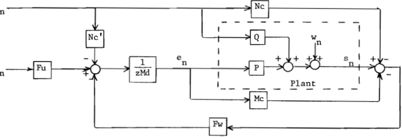
The block representation of the SISO AMAC is given by Figure 6.

v n - - - . . . , . . . - - - , - - - . . . . ; ; . t

u

n

Figure 6. SISO AMAC Representation

convolution model of the process deconvolution model of the process deterministic part of the plant

stochastic part of the plant (disturbance process) convolution model of the disturbance process

Nc' predictive convolution model of the disburbance process set point predictor

Fw unmeasured disturbances (w

n) predictor

B-2. SISO AMAC Examples

Following our presentation we will present two classical control systems used whenever the convolution and deconvolution model can be

iden-The block representation of the 5150 AMAC _{i5 given by Figure} 6.

฀฀฀฀฀฀฀฀฀฀฀฀฀฀฀฀฀฀฀฀฀฀฀฀฀฀฀฀฀฀฀

Un

Figure 6. 5150 AMAC _{Representation}

convolution model of the process

Md deconvolution model of the process

P _{deterministic part of the plant}

stochastic part of the plant (di5turbance process)

Nc convolution model of the disturbance process

Nc' predictive convolution model of the disburbance process

set point predietor

Fw _{unmeasured disturbanees (wn ) predietor}

B-2. 5150 AMAC _{฀฀฀฀฀฀}

Following our presentstion we will present two classieal control

systems used whenever the convolution and deconvolution model can be

B-2.1 The Optimum Control System of Phillipson [11]

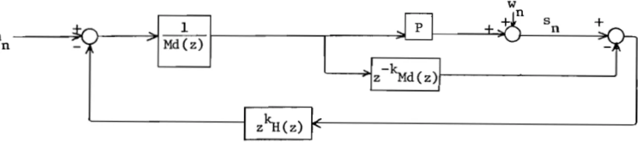
Let us suppose no measured disturbance and an asymptotically stable process with a delay of 2 samples. We take a convolution model with a delay of k samples, k underestimation of 2:

Mc(z) =

฀฀฀฀฀฀

(23)

with Md(z) supposed to have all its roots strictly in the unit circle. Then if we take a unit gain element as a set point predictor, and a

k-step-predictor

฀฀฀฀฀

for the disturbance, we obtain the optimal control system of Phillipson (Figure 7) which is an improvement over the Smith con troller.

Figure 7. Optimum Control System of Phillipson

As mentioned by Phillipson, this system used in regulation is equivalent to the Box-Jenkins-Astrom minimum-variance control [9] or to the Kalman linear regulator [12].

Thus, this system is essentially made for regulation. Moreover, the use of the inverse model as controller since this will be a high-pass filter, amplifies noise, causes violent changes in the control signal and perhaps frequent saturation. That is why the A}lAC uses here an adapted model and

B-2.1 The Optimum Control System of Fhillipson [llJ

Let us suppose no lIIeasured disrurbance and an aSYlllptotically stable

process with a delay of JI.. samples. We take a convolution model with a delay of k samples, k underestimation of

J/..:

Me(z) ""

฀฀฀฀฀฀

(23)

with Md(z) supposed to have aIL !ts roots strictly in the unit circ.le.

Then if we take a unit: gain element as a set: point: predictor. and a

k-step-predictor

฀฀฀฀฀฀

for t:he disturbance. we ob tain the opt:imal control syst:em of Fhillipson (Figure 7) which is an improvement over the Smith

con troller.

Figure 7. Optimum Control System of Phillipson

As mentioned by Fhillipson. this system uBed in regulation is equivalent

to the Box-Jenkins-Astrom minimum-variance eontrol [9] or t:o the Kalman

linear regulat:or [12].

Thus, t:his system is essentially made for regulation. Moreover, the

use of the inverse model as controller since this will be a high-pass filt:er,

amplifies noise, causes violent changes in the control signal and perhaps

30

avoids rapid changes in set point thanks to the set point predictor. Predictor H can be easily computed when the disturbance can be described as the output of a known rational filter whose input is an independent zero-mean random sequence. But to verify internal stability we must not forget the constraints on the denominator of H. Here Phillipson suggests the use of exponential smoothing for prediction to solve the problem. That way, we can answer satisfactorily the output regulation but not so properly the output tracking. The model predictive heuristic control which follows attempts to answer the two questions introducing a set point predictor and deducing the disturbance predictor.

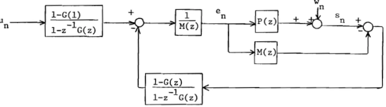
B-2.2 Model Predic tive Heuristic Control (MPHC) [13]

We give here a simplified study of this method; the very general study can be found in [14]. Suppose no measured disturbance (MPHC can

be extended to this case) and a convolution model having a moving average (MA) structure with all its roots strictly in the unit circle, we take:

M(z)

=

Mc(z)

=

Md(z)

For the set point and disturbance predictors, we choose 1- G(l)

Fu (z) = 1- z -lG(z)

(24)

(25)

where G(z) is a nonzero static gain transfer such that Fu(z) and Fw(z) satisfy stability conditions.

30

avalds rapld changes in set point thanks to the set point predictor.

Predlctor H cao be easily c01llputed when the disturbance cao be described as the output of a known rational fil ter whose input 18 an independent zero-mean random sequence. But to ver if y interna! stability we must

not forget the constraints on the denominator of H. Here Phillipson 8uggests the use of exponential smoothing for prediction ta solve the

problem. That way. ws cao suswer satisfactorily the output regulation

but not so properly the output tracking. The model predictive heuristic

control which follows attempts to auswer the two questions introducing

a set point predictor and deducing the disturbance predictor.

B-2.2 Model Predictive Heuristic Control (MPHC) [13]

We give here a simplified study of this method; the very general study can be found in [14]. Suppose no measured disturbance (MPHC can be extended to this case) and a convolution model having a moving average

(MA) structure with all its roots strictly in the unit circle. we take:

M(z) '" Mc(z) '" Md.(z)

For the set point and disturbance predictors, we choose 1- G(l)

Fu(z) - l_z-lG(z)

(24)

(25)

where G(z) 1s a nonzero statie gain transfer such that Pu(z) and Fw(z) satisfy stability conditions.

31

Then from (15) we get the MPHC law:

฀฀฀฀฀฀฀฀฀

)'M(z)'e(z)

=

--:-1-

[(l-G(l»u(z) - (l-G(z»s(z)]

1 -_{z G(z)} 1 -_{z G(z)}

(25)

(z-l)'M(z)'e(z) + s(z) = _{(l-G(l»u(z) + G(z)s(z) (26)}

Let us develop the strategy of this relation.

Both terms are similar to outputs. We call the left-hand term a predicted output sp(z) and the right-hand term a reference output sR(z), From

sp(z) = _{zM(z)e(z) + (s(z) - M(z)e(z» (27)}

we define the predicted output as the output of the model at time (n+l) corrected of the estimation w(n) of the disturbance

with sM(n+1) output of the model with a predicted input en (1). The ref-erence output sR(z) is given by a trajectory connecting the past outputs of the process to the present set point.

00 co

sR(n+1) = _{(1 -}

฀฀฀

_{gi)un +}

฀฀฀

_{gi sn-i}

Thus the MPHC strategy consists in computing future inputs such that

(29)

predicted outputs are on a connecting trajectory. Its block representation is given by Figure 8.

31

Then trom (15) we get the MPHC law:

(z - 1-

฀฀฀฀฀

) "M(z) oe(z) '" - - : - , - [(1 _ G(l))u(z) _ (1 - G(z» s(z)]

1-z G(z) 1 - z G(z)

(25)

(z-l)oM(z)"e(z)

+

s(z) m (l-G(l»u(z)

+

G(z)s(z) (26)

Let us develop the strategy of this relation.

Bath t.erms are similar ta outputs. We calI the left-hand tenu a

predicted output. sp (z) and the right-hand term a reference output sR(z),

From

Sp(Z) '"' zM(z)e(z)

+

(8(Z) -M(z)e(z» (27)

we define the predicted output as the output of the mode! at time (n+1)

corrected of the estimation Q-(n) of the disturbance

with sM(n+l) output of the mode! with a predicted input en(I). The

ref-erence output sR(z) ls given by a trajectory connecting the past outputs

of the process ta the present set point.

.

.

SR (n+1) = (1 -

฀฀฀฀

gi)Un

+

i!O gi sn-i (29)

ThuB the MPHC strategy consists in cOlIlputing future inputs such that

predicted outputs are on a connecting trajectory. rts block representation

Figure 8. MPHC Representation with G(z) as Connecting Trajectory Generator

From part A, we will satisfy the convergence criterion if M(z) has all

its roots strictly in the unit circle and (l-G(l)) is taken as the stability coefficient. But again, the transfers are not independent, for instance in a perfect modeling we have:

(30)

(31)

The regulation transfer is the discrete differentia tion of the tracking transfer. Moreover, if the model does not verify the stability condition, the strategy must be seriously questioned but i t has been extended to this case by the introduction of the notion of adapted model [14].

B-3. Choice of the Deconvolution Model

We have seen that the most general linear time invariant control law contains five independent physical components. Theoretically each can be obtained from a modeling (system or spectrum). But the deconvolution model is a special case because its use is not a physical one. We are

Un

Figure 8. MPHC Representation with G(z) as Connecting Trajectory Generator

From part: A. we will satisfy the convergence criterion if MCz) has aIl

tts roots strictly in the unit circle and CI-G(l» la taken as the stability

coefficient. But again, the transfers are not independent, for instance in a

perfect modeling we have:

Sa

Cz)

฀฀ ฀฀฀฀฀฀

(30)

Srw(z) = 1 -

฀฀฀฀฀฀฀

=

฀฀฀฀฀฀฀ ฀฀฀฀฀฀฀฀฀

SaCz) (31)

The regulation transfer 18 the discrete differentiation of the tracking

transfer. Moreover,

if

the model does not verity the stability condition, the strategy must be seriously questioned but l t has bean extended to this

case by the introduction of the notion of adapted model I14].

B-3. Choice of the Deconvolution Model

\ole _{have seen that the mast generai iinear time invariant control law}

cantains five independent physical components. Theoretically each can be

obtained from a modeling (system or spectrum). But the deconvolut:ion

33

going to show where the problem is and how to solve it.

B-3.l Terms of the Problem and Mathematical Solution Let Md(z) be this deconvolution model

Md(z) =

฀฀฀฀฀฀

(32)

with mdn(z). mdd(z) polynomials in z such that with expectation (4) degree of mdd(z) is equal to degree of mdn(z).

Mc(z) is the knowledge of the process, Le., the convolution model:

Mc(z)

=

฀฀฀฀฀฀

(33)

with mcn(z), mcd(z) polynomials in z , with degree of mcd(z) greater than degree of mcn(z). The differences between these models are in their use. Let e, s be the input and the output, we write

s(z) =

฀฀฀฀฀฀

e(z) similarly to the process, but:

e(z) =

฀฀฀฀฀฀

s I z )

is a reversed relation compared with the process.

(34)

(35)

As we want a stationary control law, following Box and Jenkins [9], we have to improve the stability of both transfers

฀฀฀฀฀฀

and

฀฀฀฀฀฀

. The former can be ensured from the stability of the process. But the

33

going ta show where the problem 15 and how ta solve it.

B-3.1

Tenus of the problem and Mathematical Solution

Let MdCz) be this deconvolution model

฀฀฀฀฀฀฀฀฀฀

(32)

with mdn(z). mdd(z) polynornials in z sueh that with expectation (4) degree

of mdclez) la

equal

ta

degree

of mdu(z).

Mc(z) la the knowledge of the pracess, Le., the convolution mode!:

฀฀฀฀฀฀฀฀฀

(33)

with men(z). mcd(z) polynomials in z, with degree of mcd(z) greater than degree of menez). The differences between these modela are in their use.

Let e,s be the input and the output, we write

s(z) =

฀฀฀฀฀฀฀

e(z) (34)

similarly ta the process, but:

e(z) -

฀฀฀฀฀฀

S(II) (35)

18 a reversed relation compared with the process.

As we want a stationary control law, fol1owing Box and Jenkins [9]. we have to improve the stabil:ity of both transfers

฀฀฀฀฀฀฀

aud

฀฀฀฀฀฀฀

• The former can bec ensured from the stability of the process. But the

latter has no physical significance and we have seen that we must impose mcn(z) to have all its roots strictly in the unit circle.

As mdd(z) has no constraint in the deconvolution use, we can take:

md(z) = mdd(z) = mcd(z) (36)

Moreover, to get a zero static gain compensator, with expression (16), we must impose:

mdn(l) = men (1) (37)

Thus the problem is: knowing the model of the process mcn(z), how to

choose mdn(z) such that i t keeps the significance of a model and i t satisfies the stability condition.

If mcn(z) has all its roots strictly in the unit circle, we take obviously:

mdn(z) = mcn(z) (38)

So the real problem occurs when mcn(z) has roots on both sides of the unit circle. Let us factorize mcn(z) into:

mcn(z) = min(z) ·mon(z) (39)

where min(z) has all its roots strictly inside the unit circle. mon(z) has all its roots strictly outside the unit circle. We don't deal with

modulus roots. As mdn(z) is used as a denominator, let us consider:

mid(z) =

฀฀฀฀฀฀

(40)

latter has no physical significance and we have seen that we must impose

menez) ta have aIL its roots strictly in the unit circle.

As mdd(z) has no constraint in the deconvolution use, we cau take:

md(z) ฀฀mdd(z) = mcdez) (36)

Moreover, ta get a zero stat:le gain compensatol.". with ฀฀฀฀฀฀฀฀฀฀฀(16), we must impose:

mIn(l) "' menel) (37)

Thus the problem is: knowing the model of the process menez), how to

choa se mdn(z) such that it keeps the significance of a mode1and i t satisfies

the stability condition.

If mcn(z) has aIL its roots strictly in the unit circle. we take

obviously:

mdn(z) = mcnez) (38)

Sa the real problem occurs when mcnez) has roots on bath sides of the

unit circle. Let us factorize mcnez) into:

mcnez) = minez) "monez) (39)

where minez) has aIL its roots strictly inside the unit circ!e, mon(z)

has aIL its roots strictly outside the unit circle. We don't deal with

unit modulus roots. As mdn(z) ls used as a denominator. let us consider: