HAL Id: hal-00275348
https://hal.archives-ouvertes.fr/hal-00275348
Submitted on 19 Dec 2017
HAL is a multi-disciplinary open access
archive for the deposit and dissemination of sci-entific research documents, whether they are pub-lished or not. The documents may come from teaching and research institutions in France or abroad, or from public or private research centers.
L’archive ouverte pluridisciplinaire HAL, est destinée au dépôt et à la diffusion de documents scientifiques de niveau recherche, publiés ou non, émanant des établissements d’enseignement et de recherche français ou étrangers, des laboratoires publics ou privés.
Chemometrics as a tool for the analysis of evolved gas
during the thermal treatment of sewage sludge using
coupled TG–FTIR
J.H. Ferrasse, Patricia Arlabosse, S. Chavez, N. Dupuy
To cite this version:
J.H. Ferrasse, Patricia Arlabosse, S. Chavez, N. Dupuy. Chemometrics as a tool for the analysis of evolved gas during the thermal treatment of sewage sludge using coupled TG–FTIR. Thermochimica Acta, Elsevier, 2003, 404 (1-2), pp.97-108. �10.1016/S0040-6031(03)00064-9�. �hal-00275348�
Chemometrics as a tool for the analysis of evolved gas during the
thermal treatment of sewage sludge using coupled TG–FTIR
J.H. Ferrasse
a,∗, S. Chavez
b, P. Arlabosse
b, N. Dupuy
caIUT de Marseille, Département de Génie Chimique—Génie des Procédés, Université Aix, Marseille 3, 13388 Marseille Cedex, France bCentre Energétique Environment, Laboratoire de Génie des Procédés des Solides Divisés, (CNRS-UMR 2392)—Ecole des Mines
d’Albi-Carmaux—Route de Teillet, 81013 Albi CT Cedex 09, France
cLaboratoire de Spectroscopie Infrarouge et Raman (LASIR), CNRS, Bˆat C5, Université des Sciences et Technologies de Lille, 59655 Villeneuve d’Ascq Cedex, France
Received 30 September 2002; received in revised form 24 January 2003; accepted 26 January 2003
Abstract
The thermal decomposition of sewage sludge has been investigated using coupled TG–FTIR for long time experiment (10 h). The exploitation of the resulted data from FTIR is performed by the SIMPLe-to-use interactive self-modelling mixture analysis (SIMPLISMA) method and allows to identify some of the evolved gases and to obtain their relative concentration profiles versus time without prior knowledge of constituents. As shown, this method can work properly for mixture with overlapped bands but some compounds remain “invisible” to FTIR analysis. More of that for long time experiment, it is possible to extract a spectrometer baseline contribution, which contributes to minimise noise and time variation.
© 2003 Elsevier Science B.V. All rights reserved.
Keywords: EGA; Mixture; Chemometric; TGA; FTIR; Sewage sludge
1. Introduction
Today, the municipal sewage sludge production rep-resents in France close to 1 million tonnes per year of dry matter, the amount of dry matter produced in Europe is estimated to be 7.7 million tonnes[1]. The stabilisation and disposal of these waste has become a problem of increasing urgency because of more re-strictive regulation of wastewater treatment, that will inevitably induce an increase in the production of sewage sludge. Thus, the sludge production in the EU is expected to increase by least at 50% by the year 2005 [2]. The thermal treatment may be
con-∗ Corresponding author. Tel.:+33-4-92-289462. E-mail address: jean-henry.ferrasse@univ.u-3mrs.fr
(J.H. Ferrasse).
sidered like an interesting route to deal with those waste.
In environmental analysis, many TA techniques have been applied to study thermal degradation of waste. For instance, Napoli used TG-DSC to analyze the degradation of refuse tires [3] and Lupascu in-vestigated the thermal characteristics of some waste agriculture products which can serve as raw materials for the production of active carbons (grape seeds, walnut shells . . . )[4]. Font studied the pyrolysis and combustion of some sewage sludges [5]. But, as the kinetics are generally complex, the elucidation of the degradation mechanisms from the knowledge of the mass variation without precise formulae for the intermediate compounds, remain rather complex.
Evolved gas analysis (EGA) is a recent and use-ful tool for the investigation of thermal decomposition
0040-6031/$ – see front matter © 2003 Elsevier Science B.V. All rights reserved. doi:10.1016/S0040-6031(03)00064-9
mechanisms as, in addition to the mass loss of the heated product, information about the evolution of the evolved substances are available. Among several tech-niques, coupling a TG with infrared spectroscopy ap-pears to be more and more common[6–11]. One major advantage of this coupling is to be a non-destructive method. Raafat uses this technique to investigate com-bustion process of fibrous sludge[12]. However, the compounds identification remains uneasy due to mix-tures. The gaseous compounds are removed by the gas carrier of the TG apparatus through a heated transfer line to the FTIR spectrometer. Thus, the spectra ob-tained are the spectra of mixtures of specific individ-ual compounds (at least the more concentrated ones). For the less concentrated ones the interpretation may be difficult according to the overlapping bands espe-cially in the water vapour region. The purpose of the present study is to identify the volatile organic com-ponents likely to be exhausted during a thermal treat-ment which is time dependant. The technique belongs to the self-modelling mixture analysis methods and is called SIMPLe-to-use interactive self-modelling mix-ture analysis, SIMPLISMA[13]. It leads to the extrac-tion of pure component spectra that contain intensity contributions from only one of the components in the mixture, with their relative concentration profiles as a function of time in our study.
The sewage sludge used in the present study as well as the TG–FTIR coupling and the operating conditions are detailed inSection 2. The SIMPLISMA method is briefly presented inSection 3.Section 4concerns the results.
2. Product and materials
2.1. Municipal sewage sludge
Municipal sewage sludge is a complex waste whose composition and physical features depend on the wastewater composition and the sludge treatment process used. It usually contains, alter mechanical dewatering, some 80% of water, 10–15% of organic compounds and 5–10% of mineral compounds.
The sewage sludge used for this study comes from the treatment plant of the town of Albi, France. The av-erage total throughput in the plant is close to 10,000 m3 a day. In comparison with the most common
treat-Table 1
Elementary composition of dry sewage sludge from Albi Dry matter (%) Carbon 36 Nitrogen 5.5 Hydrogen 5.27 Oxygen 24.5 Sulfur Undetected
ment plants in France, this sewage treatment process presents a distinctive feature: a methanation process ends the sludge treatment [14]. It is based on a bi-ological stabilisation in a liquid phase by using the mesophilic anaerobic technique. The volatile fraction of the dry matter is 69%, and the elementary compo-sition of the dry sludge is summarised inTable 1.
Before thermal analysis, the sewage sludge was pre-dried at 20◦C during 24 h in a drying oven in or-der to reduce water content to 0.1 kg of water/kg of dry matter.
2.2. The TG
Thermogravimetry (TG) was performed with a Se-taram TGA 92 [15,16]. The sample is introduced in two platinum pans of 100 !l volume (using DTA fa-cilities, but DTA is not recorded), which give an initial mass of sludge close to 125 mg. The pans undergo the following temperature program:
• a constant temperature at 20◦C during 10 min; • a temperature increase up to 120◦C with 5 K/min; • a constant temperature for 5 h at 120◦C;
• a new temperature ramp up to 350◦C with
10 K/min;
• an isotherm of 5 h at 350◦C.
This unusual temperature profile is used to be the closest to an industrial thermal treatment planned. 2.3. FTIR
IR measurements were performed with a Perkin-Elmer FTIR 2000, using a KBr cell maintained at 200◦C. The measurement cell is continuously purged with nitrogen. The resolution was 2 cm−1 with two accumulations per spectra. The interval between two measurements is equal to 14.6 s.
2.4. The TG–FTIR coupling
A heated line furnished by Perkin-Elmer makes the physical coupling between the thermal analyser and the spectrometer. This line is maintained at a temper-ature of 200◦C. All care must be taken to avoid cold points. A Teflon liner assures gas transport into the heated line. This liner is placed directly in the bot-tom of the furnace and temperature is close to 200◦C (a map of temperatures of the furnace was previously generated with a thermocouple).
Air, previously purged with a Whatman purifier, was used as sweeping gas. The flow rate was close to 1.75 l/h. Delay time from furnace to gas cell is esti-mated to be close to 10 min using plug flow approach.
3. SIMPLISMA approach
The method used for self-modelling analysis is the SIMPLISMA approach[13]. The great advantage of this method resides in the fact that it uses a relatively simple algorithm. All the intermediate steps are dis-played in the form of spectra that makes SIMPLISMA usable without extensive knowledge of the calculation procedures behind it. The mathematical principle of SIMPLISMA is based on the presence of pure vari-ables. In spectroscopic terms, a pure variable (e.g. a wavelength for absorption electronic spectra) is a vari-able that has intensity contribution from only one of the components of the mixture. When the pure vari-ables of all the components are known, it is possible to calculate the spectra of the pure components from the mixture spectra. The pure variables can be determined by mathematical means without prior knowledge of the pure components (seeAppendix A). SIMPLISMA is then a powerful tool to determine the pure variables followed by the calculation of the pure spectra and their associated “contributions”.
Some applications of SIMPLISMA have already been reported in the literature on FT-Raman spectra of hydrogen peroxide activation by nitriles time-resolved reaction[18], FT-IR microscopy spectra of polymer laminate and pyrolysis mass spectra of biomaterials (feedstock)[19,20]and for LC/MS data[20]. For more information, Gemperline and Hamilton[21,22]wrote complete articles about factor analysis based on mix-ture analysis, and for a more geometrically oriented
explanation, see the review of Windig[23]about mix-ture analysis by multivariate methods.
In order to obtain proper resolution of the mixture data, user interaction is possible. This requirement is a plus in order to deal properly with features such as noise, peak shift and instrument drift[24]. In this study, only the offset was modified (see Appendix A
for the meaning of this parameter).
4. Results and discussion
From an experimental test, we obtain a TG curve and an FTIR data set composed of 2646 infrared spec-tra. The information content in this data is consider-able, and thus the exploitation is difficult and memory problems occurs for computers. That is why we decide to divide the whole data set into several zones.
Fig. 1presents the mass loss of the studied sewage
sludge as a function of time (TG curve) and the evo-lution of the sludge temperature using DTA facilities from the apparatus.
The variations in the slope of TG curve express the evolution of sludge degradation rate. Following these variations, the whole data set are divided into five zones:
• zone I: between 0 and 26 min, spectra from 41 to 146 (the spectra numbered 1–40 are not included in this analysis because they correspond to the delay time between the furnace and gas cell);
• zone II: between 26 and 327 min, spectra from 146 to 1386;
• zone III: between 327 and 348 min, spectra from 1386 to 1471;
• zone IV: between 348 and 470 min, spectra from 1471 to 1975;
• zone V: between 470 and 643 min, spectra from 1975 to 2646.
Fig. 2presents a spectrum of each zone described
above. As we can see, intensities of the water vapour and the carbon dioxide spectra prevent the identifica-tion of other compounds on the raw data set.
4.1. Zone I
This zone corresponds to the first temperature climb from 20 to 120◦C. The 105 spectra of this zone were
Fig. 1. TG curve and temperature profile of the experiment as a function of time.
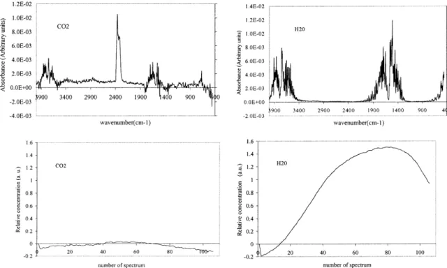
treated using the SIMPLISMA procedure with an off-set equal to 4 (seeAppendix Afor the meaning of this offset). This analysis yields two typical spectra cor-responding to water and carbon dioxide traces. The resolved spectra and their relative contributions are shown inFig. 3. As a matter of fact, the relative con-centration profiles show that water was the prevail-ing component and its highly concentration explained the difficulty to obtain a good extraction of the wa-ter spectra. Some residues of its rotational structure were observed on the CO2 spectra. The difference of
purge time between the reference spectrum (5 min) and the sample one could explain the negative value of
Fig. 2. Example of a instantaneous spectrum of the mixture for each selected zone.
the relative concentration (10–20 min). When the con-centrations of the compound are very small, negative concentrations are founded because the infrared cell contained more water and CO2 in the reference time
than in the sample one. This zone exactly corresponds to the first increase of temperature from 25 to 120◦. The mass loss corresponds to 10% of the initial mass, and we may conclude that this is essentially drying. 4.2. Zone II
This zone corresponds to the first temperature stage at 120◦C. The SIMPLISMA analysis performed on
1240 absorbance spectra (offset = 15) shows that four components could be extracted: spectrometer contribution, water, carbon dioxide and ammonia (water residues are observed in CO2 and NH3
spec-tra). The spectrometer contribution was normal from a spectroscopic point of view. As a matter of fact, the spectrometer caused time variations according to the room temperature, the source energy, etc. So if the analysis is time consuming, the reference spectrum is not sufficient to eliminate some spectral varia-tions. Consequently a contribution named “baseline or spectrometer contribution” is extracted, consider-ing a wavelength equal to 4000 cm−1. The departure of water, which corresponded to the end of drying, appeared at the first plateau. Then, the relative con-centration attributed to water became very weak, like those of carbon dioxide. During this stage, the mass loss is close to 0.6% of the initial mass and it seems to come only from NH3production as can be seen in
Fig. 4. The oscillations in the concentration profiles
can be related to a difference in the purge system, in particular to the compressor pump period.
4.3. Zone III
This is a short transition zone that corresponds to the second temperature climb from 120 to 350◦C. Only three components could be extracted using SIM-PLISMA (offset = 15): spectrometer contribution, water and CO2. The relative concentrations of water
and CO2(Fig. 5) are negatives at the beginning of this
stage according to the spectra which presented nega-tives absorbance. From 334 min, the relative concen-tration of CO2 increases weakly and simultaneously
the mass loss on the TG curve starts to decrease again. At the end of this zone, approximately 30% of the initial mass of sludge was consumed. The temperature of sludge at the same moment (280◦C) corresponds to the minimum level of energy to trigger off the re-action. Indeed, only the presence CO2 was detected
by FTIR but we can suppose that some other gases such as H2, O2, etc. which are inactive in infrared, are
simultaneously produced[25]. 4.4. Zone IV
In order to identify all the gases during this step, the SIMPLISMA approach was performed on 504
spec-tra with an offset equal to 4. Twelve specspec-tral con-tributions were extracted corresponding to pure vari-ables at 2364, 1508, 964, 4000, 2936, 2072, 1060, 1740, 712, 1800, 2180 and 3016 cm−1. These variables were respectively attributed to carbon dioxide, wa-ter, ammonia, spectrometer contribution, ethane, car-bonyl sulfide, methanol, unknown organic product, hydrogen cyanide, acetic acid, carbon monoxide and methane. The products were identified according to the Shimanouchi interpretation [26] or by compari-son with the spectra ones of the NIST standard ref-erence database [27]. The pure variable extracted at 4000 cm−1is a representation of the spectrometer con-tribution identified by SIMPLISMA as a pure product. Instead of showing all the spectra, pure variables and associated peaks are compared to literature value in
Table 2.
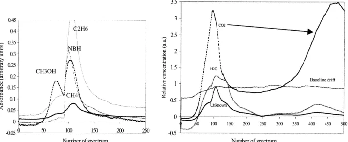
The concentration profiles (Fig. 6) associated to the SIMPLISMA pure components show that some species, such as NH3, CH4, C2H6 and CH3OH, are
strongly found at the beginning of the process, while others like H2O, CO2 are produced all the time with
different concentration ratios. These concentration profiles show the existence of two peaks of maximal concentration of the compound. The first one appears at 372 min (close to 107 on abscissa ordinate) and is generally the most intense. The second one appears close to 461 min (470 on the abscissa ordinate) and the intensity may be variable according to the component. During this stage, a thermal effect (disturbing sample temperature measurement) is register too (at 419 min), as well as a total mass loss of 21.4%, shown
onFig. 1. However, this mass loss is fickle and an
ac-celeration of the sludge degradation rate is registered at 439 min.
Beside this, water and dioxide carbon are synony-mous with combustion. Combustion is an exothermic oxidation reaction of organic matter, which needs a minimal thermal contribution to produce water, carbon dioxide and some by-products (according to the exper-imental conditions). Carbon monoxide is a by-product of combustion produced under sub-stoichiometric con-ditions or when the temperature is not high enough to lead the instantaneous oxidation of CO into CO2.
Some of those by-products (methane, alcohol, acetic acid) have been also identified in sludge pyrolysis (a thermal treatment in sub-stoichiometric conditions) by Conesa[25]with a TG–MS coupling.
Table 2
Comparison between the extracted pure spectra and the literature data Pure variable
2364 cm−1 1508 cm−1 964 cm−1 4000 cm−1 2936 cm−1 2072 cm−1 Exp. Lit. Exp. Lit. Exp. Lit. Exp. Exp. Lit. Exp. Lit.
672 671 1600 1595 948 943 2968 2064 2063 P P P P P P P 2900 D D 2352 2360 3237 3745 2868 1462, 829 D D P P 1620 1626 BASELINE ND 3668 3662 FB FB 3328 3326 DRIFT Product CO2 H2O NH3 C2H6 COS 1060 cm−1 1740 cm−1 712 cm−1 1800 cm−1 2180 cm−1 3016 cm−1 1032 1033 712 712 2140 2145 3016 3017 TB TB 1144 P P 980 988 D D P P 1345 3308 3311 1304 ND D D 1176 1177 ND 2960 2960 2096 P P 1564 ND 1276 1280 3680 3680 1740 1392 1392 1792 1799 D D
Product CH3OH Unknown HCN CH3COOH CO CH4
P stands for pattern, D for doublet, TB for three bands, FB for four bands, ND for non-detected.
Indeed, at the beginning of this stage, we observe the combustion of sludge, associated with some other re-actions that will simultaneously produce the whole of the components identified. These transformations will
Fig. 6. Relative contribution profiles from zone IV.
consume around 4% of the initial mass of sludge with a maximum on the reaction rates at 373 min. Proba-bly, the heat produced during combustion increase the sludge temperature and induces the acceleration of the
reaction rates. As a consequence, a variation on the slope of the TG curve and the appearance of the sec-ond peak on the relative concentration of CO, H2O,
CO2 is registered. This zone emphasises the helpful
tool. Indeed, the peak’s identification done here has to be compared to the apparent spectra of zone IV shown inFig. 2.
4.5. Zone V
This is the end of the stage at 350◦. The SIM-PLISMA approach was performed with an offset of 28. H2O, CO2, spectrometer contribution, HCN, CO and
NH3were found. Relative concentration profiles show
a decreasing slope that can be linked to the TG curves. This one does not show a stabilisation of the mass. This stage corresponds to the end of the combustion. This tends prove that even in slow combustion rate, the exhausted gas obtained are not only composed by CO2and H2O but also of some pollutants as CO, NH3,
HCN.
At the end of this treatment, the loss of mass calculated on a dry basis is close to 58% of the initial dry matter. Compared to the 69% of whole volatile fraction, this low temperature treatment
Fig. 7. Reconstruction of the CO2relative concentration profile on the whole experiment.
gives up to a total conversion of 84% of the organic matter.
4.6. Reliability of the results
The exploitation of the spectra was made on five zones according to the TG curve, which allowed the identification of components. Once the pure vari-ables have been selected, data sets can be resolved into pure infrared spectra and their contributions in the original spectra. After the resolution of the pure components spectra, an associated pure contributions matrix is deduced by writing the raw data matrix as the product of the unknown matrix containing the contributions of the pure infrared spectra in the mix-ture spectra with the normalised matrix containing the pure component infrared spectra previously re-solved. So, the concentration profiles were obtained separately. In order to verify the reliability of the concentrations given by SIMPLISMA, the profile of carbon dioxide is rebuilt all along the experiment. The result is given in Fig. 7 in which we can see that the scale of size was respected, even if some shifts could be seen at the borders of the different zones.
5. Conclusions
The TGA–FTIR coupling appears to be a very use-ful tool to study the thermal decomposition of sewage sludge. Previous results show that the infrared spectra are quite different all along the experiment and that they are characterised by large amount of water and carbon dioxide. But, the complete identification of the lower concentration products needs the use of statis-tical methods like SIMPLISMA, specially in the zone IV, where up to 11 compounds could be found despite overlapping bands. Long period acquisition has been done with a short time interval between spectra.
The associated concentration profiles obtained led to consider that it is possible to use this experimental set up to study thermal treatment. This study should conduct to the optimisation of the process operating conditions in terms of security and environmental pro-tection.
In addition, at the beginning of the second isother-mal stage (at 350◦C) a step of combustion was deduced from the identification of the set of 11 com-ponents. Also, the determination of the kinetics of sludge decomposition can be envisaged by the use of TGA–FTIR coupling and associated contribution profiles from SIMPLISMA could be helpful.
However, a limitation of this method was illustrated in zone III by the non-justification of close to 35% of the mass loss. For the moment, this can be inter-preted as the production of infrared-spectroscopy in-active species but more analysis must be conducted, perhaps by using a GS or MS apparatus since FTIR does not deteriorate the gas phase. As a matter of fact, chemometric could also be used for those techniques.
Acknowledgements
The authors thank Drs. W. Windig and J. Guilment for helpful discussions and advice to use SIMPLISMA software. This work was partially supported by the French “Region Midi-Pyrénées”.
Appendix A. Theory of the SIMPLISMA mathematical treatment
As explained before, the SIMPLISMA approach is based on the concept of pure variables. A pure variable
is a variable that has intensity contributions from only one of the components of the mixture; in mathematical terms it is a variable with the maximum ratio of the standard deviation to the mean. This ratio is called the purity ratio and is given by the expression:
Pij= Wij× ! σi µi+ α " (A.l) In this equation, Pij is the purity value of the
vari-able (i is the varivari-able index), from which the jth pure variable will be selected and represent the mean and the standard deviation of the variable i. The constant α is added to give pure variables with a low mean value (i.e. in the noise range) a lower purity value Pij
and is called offset. Typical values for α range from 1 to 5% of the maximum of µi The weight factor Wij
is a determinant-based function that corrects for pre-viously chosen pure variables. The value of Wij also
depends on the value of α. The purity values are rep-resented in the form of spectra. Along with the purity spectrum, the standard deviation spectrum is available, described byEq. (A.2):
Sij= Wij× σi (A.2)
This spectrum has more similarities with the orig-inal spectrum and is used to facilitate the validation of the pure variables. The interactive process makes it possible to guide the pure variable selection by chang-ing the value of α in combination with the option to exclude certain spectral ranges for the selection of pure variables. This capability is especially useful since pure variables may describe unwanted features in the data set.
Once the pure variables have been determined, the data set can be resolved into the pure components and their contributions in the original spectra. The task of the mixture analysis is to express the dataset as a product of a matrix containing the concentrations and a matrix containing the spectra of the pure components:
D= CR (A.3)
D is the matrix with the original data; its size is cv, where c is the number of cases (spectra) and v the number of variables (wavelength). The matrix C (size cn, where n is the number of pure components) con-tains the concentration of the pure components in the mixtures. The matrix R (size nv) contains the resolved spectra.
Because pure variables are directly proportional to the concentrations of the pure components, their in-tensities can be used in the matrix C, and since the matrix D is known, the matrix R of the pure compo-nents can be calculated. Although the pure variable intensities can be used directly (after a normalisation step) to calculate the concentrations, it is better to use the newly calculated R in combination with D to cal-culate C. The thus, obtained concentrations are in fact a projection of the second derivative of the pure vari-able intensities on the original data set. For details about the procedure to calculate the spectra and con-centrations see[13], for comparison of SIMPLISMA with other principal component analysis methods, see
[17].
References
[1] J.E. Hall, Chem. Indus. 6 (1993) 188.
[2] A. Midilli, M. Dogrout, C. Howarth, M. Ling, T. Ayhan, Energy Conv. Manage. 42 (2000) 157.
[3] A. Napoli, Ph.D. Thesis, Université Paul Sabatier de Toulouse, France, 1998.
[4] T. Lupascu, I. Dranca, V.T. Popa, M. Vass, J. Thermal Anal. Calorim. 63 (2001) 855.
[5] R. Font, A. Fullana, J.A. Conesa, F. Llavador, J. Anal. Appl. Pyrolysis 58–59 (2001) 927.
[6] W.M. Groenewoud, W. de Jong, Thermochim. Acta 286 (1996) 341.
[7] P. Antonetti, Ph.D. Thesis, Université de Provence, France, 1999.
[8] C.A. Wilkie, Polym. Degrad. Stab. 66 (1999) 301.
[9] W. Geyer, F.A.-H. Hemidi, L. Brüggemann, G. Hanschmann, Thermochim. Acta 361 (2000) 139.
[10] M. Wesolowski, M. Czerwonka, P. Koniezynski, Thermochim. Acta 323 (1998) 159.
[11] J.P. Gibert, J.-M. Lopez Cuesta, A. Bergeret, A. Crespy, Polym. Degrad. Stab. 67 (2000) 437.
[12] G.R. Saade, J.A. Kozinski, Biomass Bioenergy 18 (2000) 391. [13] W. Windig, G. Guilment, Anal. Chem. 63 (1991) 1425. [14] C. Couturier, S. Berger, I. Meiffreu (Eds.), Agence de l’eau
Audur-Garonne et Solagro, 2001.
[15] Handbook of Thermal Analysis and Calorimetry, Elsevier, Amsterdam, 1998.
[16] W. Wendlandt, Thermal Analysis, third ed., Wiley, 1985. [17] W. Windig, J.L. Lippert, M.J. Robbins, K.R. Kresinske, J.P.
Twist, A.P. Snyder, Chemometr. Intell. Lab. Sys. 9 (1990) 7. [18] V. Vacque, N. Dupuy, B. Sombret, J.P. Huvenne, P. Legrand,
Appl. Spectrosc. 51 (1997) 407.
[19] W. Windig, D.A. Stephenson, Anal. Chem. 64 (1992) 2735. [20] W. Windig, W.F. Smith, W.F. Nichols, Anal. Chim. Acta 446
(2001) 467.
[21] P.J. Gemperline, J. Chemometr. 3 (1989) 549.
[22] J.C. Hamilton, P.J. Gemperline, J. Chemometr. 4 (1990) 1. [23] W. Windig, Chem. Int. Lab. Sys. 4 (1998) 201.
[24] L.A. Currie, L.J. Gleser, Chem. Int. Lab. Sys. 10 (1991) 59. [25] J.A. Conesa, A. Marcilla, R. Moral, J. Moreno-Caselles, A.
Perez-Espinoza, Thermochim. Acta 313 (1998) 63. [26] T. Shimanouchi, Tables of Molecular National Bureau of
Standards, 1972, pp. 1–160.
[27] Data from NIST Standard Reference Database 69, NIST Chemistry WebBook, February 2000 Release, 2000.