HAL Id: tel-00624419
https://tel.archives-ouvertes.fr/tel-00624419
Submitted on 16 Sep 2011
HAL is a multi-disciplinary open access
archive for the deposit and dissemination of
sci-entific research documents, whether they are
pub-lished or not. The documents may come from
teaching and research institutions in France or
abroad, or from public or private research centers.
L’archive ouverte pluridisciplinaire HAL, est
destinée au dépôt et à la diffusion de documents
scientifiques de niveau recherche, publiés ou non,
émanant des établissements d’enseignement et de
recherche français ou étrangers, des laboratoires
publics ou privés.
Modélisation mathématique de la contagion de défaut
Andreea Minca
To cite this version:
Andreea Minca. Modélisation mathématique de la contagion de défaut. Mathématiques [math].
Université Pierre et Marie Curie - Paris VI, 2011. Français. �tel-00624419�
UNIVERSITÉ PIERRE ET MARIE CURIE
ÉCOLE DOCTORALE DE PARIS CENTRE
THÈSE
pour obtenir le titre de
Docteur en Mathématiques Appliquées
de l’Université Pierre et Marie Curie
Présentée par
Andreea Catalina Minca
Modélisation mathématique de la
contagion de défaut
Mathematical modeling of financial contagion
Préparée sous la direction de
Rama
CONT
Soutenue publiquement le 5 Septembre 2011
devant le jury composé de :
M. Marco AVELLANEDA
(Rapporteur)
M. Rama CONT
M. Stéphane CREPEY
(Rapporteur)
M. Michel CROUHY
M. Gilles PAGES
Mme Agnès SULEM
Mlle Emily TANIMURA
i
Résumé
Cette thèse porte sur la modélisation mathématique de la contagion de défaut. Un choc éco-nomique induit des pertes initiales, de là le défaut de quelques institutions est amplifié par des liens financiers complexes ce qui engendre alors des défauts à large échelle. Une première approche est donnée par les modèles à forme réduite. Les défauts ont lieu en fonction des ins-tants d’arrivée d’un processus ponctuel marqué. On propose une approche rigoureuse de la calibration des modes “top down” pour les dérivés de crédit multi noms, en utilisant des mé-thodes de projection Markovienne et de contrôle d’intensité. Une deuxième approche est celle des modèles structurels de risque de défaut. On modélise spécifiquement les liens économiques qui mènent à la contagion, en représentant le système financier par un réseaux de contreparties. Les principaux types de contagion sont l’illiquidité et l’insolvabilité. En modélisant le réseau financier par un graphe aléatoire pondéré et orienté on obtient des résultats asymptotiques pour la magnitude de la contagion dans un grand réseau financier. On aboutit à une expression analytique pour la fraction finale de défauts en fonction des caractéristiques du réseau. Ces ré-sultats donnent un critère de robustesse d’un grand réseau financier et peuvent s’appliquer dans le cadre des stress tests effectués par les régulateurs. Enfin, on étudie la taille et la dynamique des cascades d’illiquidité dans les marchés OTC et l’impact, en terme de risque systémique, dû à l’introduction d’une chambre de compensation pour les CDS.
Mots clés : Risque systémique, contrôle d’intensité, réseaux financiers, graphes aléatoires, contagion de défaut, chambres de compensation.
ii
Abstract
The subject of this thesis is the mathematical modeling of episodes of default contagion, by which an economic shock causing initial losses and defaults of a few institutions is amplified due to complex financial linkages, leading to large scale defaults. A first approach is represented by reduced form modeling by which defaults occur according to the arrival times of a marked point process. We propose a rigorous approach to the calibration of “top down” models for portfolio credit derivatives, using Markovian projection methods and intensity control. A second, more ambitious approach is that of structural models of default risk. Here, one models specifically the economical linkages leading to contagion, building on the representation of the financial system as a network of counterparties with interlinked balance sheets. The main types of financial distress that cause financial failure are illiquidity and insolvency. Using as underlying model for a financial network a random directed graph with prescribed degrees and weights, we derive asymptotic results for the magnitude of balance-sheet contagion in a large financial network. We give an analytical expression for the asymptotic fraction of defaults, in terms of network characteristics. These results, yielding a criterion for the resilience of a large financial network to the default of a small group of financial institutions may be applied in a stress testing framework by regulator who can efficiently contain contagion. Last, we study the magnitude and dynamics of illiquidity cascades in over-the-counter markets and assess the much-debated impact, in terms of systemic risk, of introducing a CDS clearinghouse.
Keywords:Systemic risk, intensity control, financial networks, random graphs, default con-tagion, clearing house.
iii
Remerciements
J’ai une profonde gratitude envers mon directeur de thèse Rama Cont, qui durant les dernières quatre années, a complètement changé la trajectoire de ma carrière. Je le remercie pour m’avoir suggéré un sujet nouveau et passionnant, pour m’avoir appris à veiller continûment à la fois au réalisme mais aussi à la rigueur mathématique. Merci de m’avoir fait confiance!
Je remercie également Agnès Sulem pour m’avoir accueillie dans son équipe à l’INRIA. J’ai bénéficié de son soutien et de ses judicieux conseils. Une jeune femme en début de carrière ne pourrait pas avoir meilleur modèle que vous!
Je suis très reconnaissante envers Marco Avellaneda et Stéphane Crepey qui m’ont fait l’honneur d’être rapporteurs de ma thèse. Leurs remarques precieuses m’ont permis d’améliorer la présentation finale de mon manuscrit. Je les remercie pour leur gentillesse et la rapidité, malgré leur programme chargé, dont ils ont fait preuve pour envoyer leurs rapports. Je remercie chaleureusement Agnès Sulem, Michel Crouhy, Gilles Pagès et Emily Tanimura pour avoir accepté de faire partie de mon jury et pour l’intérêt qu’ils ont porté à mon travail.
Je tiens à remercier Michel Crouhy, qui m’a toujours appuyée dans mes démarches ainsi que la Fondation Natixis pour la Recherche Quantitative pour avoir sélectionné mon projet de thèse et avoir soutenu mon travail. A l’INRIA, j’ai eu la chance de bénéficier des échanges scientifiques avec Agnès Sulem et Jean Philippe Chancelier lors de notre groupe de travail sur le contrôle du risque systémique.
Merci aux collègues de LPMA grâce à qui mon travail s’est déroulé dans une belle ambiance. Merci à Sophie, Cyril, Reda et Karim, à la “famille Rama”, Amel, Lakshithe, Adrien et Amal pour leur amitié et les beaux moments qu’on a pu partager!
Une pensée à Jacques Portès, Corentin, Isabelle et Josette.
Je suis reconnaissante envers mes professeurs de Paris 6, et tout particulièrement Nicole El Karoui et Gilles Pagès, qui ont encadré ma formation en finance pendant le DEA.
Les dernières lignes de ces remerciements vont à ma famille : ma mère Angela, mon père Marian et ma soeur Anca. C’est grâce à leur sacrifices et leur encouragements que j’en suis arrivée là. Enfin, je remercie infiniment Hamed, c’est grace à toi et à ton soutien dans les moments difficiles que j’ai pu parcourir ce bout de chemin que represente la thèse. Merci de m’avoir donné le courage!
Contents
I Overview 1
1 Reduced form modeling of portfolio credit risk . . . 2
1.1 Credit derivatives: CDSs and CDOs . . . 3
1.2 Pricing of portfolio credit derivatives . . . 3
1.3 The inverse problem of reconstructing the portfolio default intensity . . 4
2 Structural modeling of default contagion: the network approach . . . 6
2.1 Financial linkages and domino effects . . . 7
2.2 Distress propagation in a financial network . . . 8
2.3 Random financial network models . . . 16
3 Contributions of the thesis . . . 20
3.1 Contributions of Chapter II . . . 20
3.2 Contributions of Chapter III . . . 21
3.3 Contributions of Chapter IV . . . 25
3.4 Contributions of chapter V . . . 25
4 Publications and Working Papers . . . 26
II Reconstruction of portfolio default intensities 27 1 Introduction . . . 28
2 Portfolio credit derivatives . . . 29
2.1 Index default swaps . . . 30
2.2 Collateralized Debt Obligations (CDOs) . . . 30
2.3 Top-down models for CDO pricing . . . 31
3 Identifiability of models from CDO tranche spreads . . . 33
3.1 Mimicking marked point processes with Markovian jump processes . . . 34
3.2 Information content of portfolio credit derivatives . . . 36
3.3 Forward equations for expected tranche notionals . . . 37
4 The calibration problem . . . 38
4.1 Point processes and intensities . . . 38
4.2 Formulation via relative entropy minimization . . . 40
4.3 Dual problem as an intensity control problem . . . 42
4.4 Hamilton Jacobi equations . . . 44
4.5 Handling payment dates . . . 46
5 Recovering market-implied default rates . . . 47
5.1 Calibration algorithm . . . 47
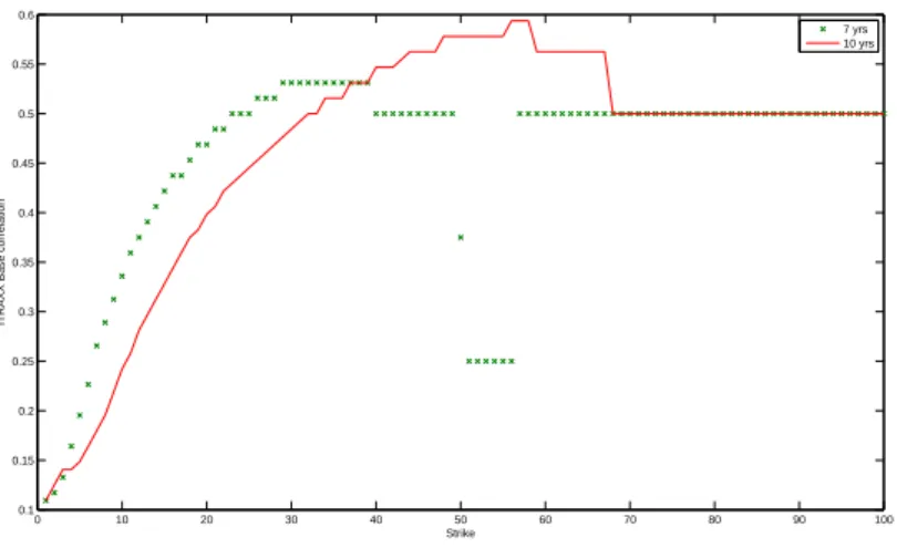
5.2 Application to ITRAXX tranches . . . 48
6 Conclusion . . . 51
III Resilience to contagion in financial networks 53 1 Introduction . . . 54
1.1 Summary . . . 55
vi Contents
2 A network model of default contagion . . . 58
2.1 Counterparty networks . . . 58
2.2 Default contagion . . . 59
2.3 A random network model . . . 59
2.4 Link with the configuration model . . . 60
3 Asymptotic results . . . 62
3.1 Assumptions . . . 62
3.2 The asymptotic magnitude of contagion . . . 65
4 Resilience to contagion . . . 66
4.1 A simple measure of network resilience . . . 66
4.2 Relation with the Contagion threshold of a graph . . . 69
5 Contagion in finite networks . . . 70
5.1 Relevance of asymptotics . . . 70
5.2 The impact of heterogeneity . . . 72
5.3 Average connectivity and contagion . . . 72
6 Appendix: proofs . . . 74
6.1 Coupling . . . 74
6.2 A Markov chain description of contagion dynamics . . . 76
6.3 A law of large numbers for the contagion process . . . 78
6.4 Proof of Theorem 3.8 . . . 81
6.5 Proof of Theorem 4.3 . . . 83
IV Stress Testing the Resilience of Financial Networks 87 1 Introduction . . . 87
2 Size of default cascade . . . 89
3 Stress testing . . . 90
3.1 Stress testing resilience to macroeconomic shocks . . . 91
3.2 An example of infinite network . . . 92
3.3 A finite scale-free network . . . 95
4 Discussion . . . 97
V Credit Default Swaps and Systemic Risk 99 1 Introduction . . . 100
2 Over-the-counter markets . . . 101
2.1 OTC derivatives: notional, mark-to-market and daily variations . . . 102
2.2 Concentration in OTC markets . . . 103
3 A network model for OTC derivatives receivables . . . 105
3.1 Illiquidity cascades . . . 107
4 A random network model for OTC markets . . . 109
4.1 A random model for a (non CDS) exposure network . . . 110
4.2 A random CDS network model . . . 111
5 Resilience to illiquidity cascades under a stress test scenario . . . 112
6 Numerical results . . . 114
6.1 The stress test scenario . . . 114
6.2 A sample OTC network . . . 115
Contents vii
7 Conclusions . . . 120
8 Appendix: pricing portfolios with collateral and counterparty risk . . . 122
8.1 Cash flows of collateralized CDS . . . 122
8.2 Pricing of CDS . . . 123
Chapter I
Overview
Since the onset of the financial crisis in 2007, more than 370 of the almost 8000 US banks insured by the Federal Deposit Insurance Corporation have failed. By comparison, between 2000 and 2004 there were around 30 failures and no failures occurred between 2005 and the beginning of 2007.
The subject of this thesis is the mathematical modeling of such episodes of default contagion, by which an economic shock causing initial losses and defaults of a few institutions is amplified due to complex financial linkages, leading to large scale defaults.
Drawing a parallel with single name credit risk models we can distinguish between two classes of default contagion models.
An approach, commonly used in credit risk management, is represented by reduced form models. Here one regards firms as an ensemble of names in a portfolio and models the probability of defaults in this portfolio. Defaults occur according to the arrival times of a marked point process, where the mark determines the loss in the portfolio upon default. Clearly, capturing contagion effects depends in reduced form models on the ability of the underlying point process to exhibit clusters. In this sense, more recently, self exciting processes like time-changed birth processes and Hawkes processes have been proposed as a way to model default contagion [71, 60].
A second, more ambitious approach is that of structural models of default risk. Here, one models specifically the economical linkages leading to contagion, building on the representation of the financial system asa network of counterparties with interlinked balance sheets. The main types of financial distress that cause financial failure are illiquidity and insolvency. Illiquidity occurs when the liquidity reserves at a certain time cannot cover the payment obligations at that time, whereas insolvency means that the total value of the banks’ liabilities exceeds the total value of assets. Propagation of financial distress is modeled via domino effects: a shock (which may be a liquidity shock or a loss in assets’ value) affecting balance sheets of a few institutions will propagate due to interconnectedness to neighboring institutions and may possibly affect an important fraction of the financial system. The acknowledgement of bank’s interconnectedness and the associated contagion mechanisms has led to an increased advocacy to account for network effects when discussing regulatory requirements [84, 85, 47, 37], be it for liquidity or capital.
Thedifference between these classes of models lies primarily in the information set available to the modeler. Structural models of contagion rely on a large set of information on balance sheets and the interrelations between those balance sheets. On the other hand, reduced form models rely on a much smaller information set, for example the market information. Therefore,
2 Chapter I. Overview the scope of these two classes of models is different. First, as argued in [97], for pricing and hedging of derivatives, the relevant set of information is the market information, since this set of information is used by market participants to determine prices. In this case, the reduced form modeling is appropriate. On the other hand, the relevant set of information available to a regulator is much more detailed, containing information on the composition of balance sheets, the degree of interconnectedness of each bank, etc. As such, for regulatory purposes -for example identifying sets of banks which pose the highest systemic risk, setting regulatory minimal ratios of liquidity and capital, rendering a network resilient to contagion - the network approach is natural.
This introductory chapter is organized as follows. In Section 1, we summarize the main elements of our framework of Chapter II for reconstructing the default intensity in a portfolio from market prices of credit derivatives referencing the respective portfolio. The calibration problem can be formalized in terms of minimization of relative entropy with respect to a given prior under calibration constraints. The dual problem is shown to be an intensity control prob-lem, characterized in terms of a HJB system of differential equations, for which an analytical solution can be found.
Then, passing to the structural approach, Section 2 describes the economical mechanisms that can lead to a system level contagion like the financial crisis we have witnessed. We identify different types of linkages that transmit financial distress across institutions. In Section 2.2 we introduce a detailed model of balance sheets, that allows for joint modeling of insolvency and illiquidity cascades on the financial network. In Section 2.3, we introduce two classes of weighted random graphs that will serve us as models of financial networks throughout this thesis. Last, Section 3 summarizes the original contributions of this thesis.
1
Reduced form modeling of portfolio credit risk
A model of portfolio credit risk is specified by a filtration that represents the set of observable pieces of information, a default process counting the credit events in the portfolio and the distribution of losses at these credit events [78]. When the model is intended for pricing and hedging, the set of observable pieces of information is the market information and in most cases default time is inaccessible [97]. This is the assumption made in reduced form models, where defaults arrive according to a point process with a continuous compensator. The literature of reduced form modeling for portfolio credit risk can be traced back to Kusuoka [102], Davis and Lo [57] and Jarrow and Yu [98]. One approach is the so-called bottom up approach, where one models the default intensity for each name in the portfolio while specifying a dependence structure between these processes. Besides the previously cited papers, other examples include [39, 62, 56, 125]. The other approach, is the so-called top-down approach, where one models directly the intensity of the aggregate loss process [32, 124, 77, 71, 10, 108, 60]. While top down models lose the information on the identity of the defaulted names, they have an important gain in analytical tractability, in particular regarding calibration to market prices. We contribute to this literature by introducing a non-parametric algorithm for calibration of top-down models. We begin this section by giving some background on credit derivatives. Then, we briefly discuss pricing of portfolio credit derivatives, and finally precise our contributions to this literature.
1. Reduced form modeling of portfolio credit risk 3
1.1 Credit derivatives: CDSs and CDOs
The simplest credit derivative is a credit default swap (CDS). A CDS is a contract between two parties, a protection buyer and a protection seller, having a third party a as reference entity. Upon the default of the reference entity, the protection buyer receives a payment equal to the notional N(a) of the swap, times the loss given default 1− R(a) of the reference entity. The
quantity R(a) is known as the recovery rate of the entity a: how much will this entity be able to repay its creditors for one dollar of debt. In return, the protection buyer pays a premium, equal to an annual percentage X of the notional, to the protection seller. The premium X is called the CDS spread. This spread is paid until either maturity is reached or default occurs.
Consider now a portfolio of N reference entities and let us denote by τ (1) < τ (2) <· · · < τ (N ) the ordered default times of these entities. The underlying process of this portfolio is the piecewise constant loss process
Lt=
X
τk≤t
N(k)(1
− R(k)), (I.1)
where N(k) and R(k) denote here the notional and respectively the recovery rate of the k-th
entity to default.
Investors, depending on their risk appetite, seek exposure to a certaintranche or interval. The CDO is decomposed in a set of I tranches: {[Ki, Ki+1]}I−1i=0 with K0 = 0 and KI = 1.
An investor in the i-th tranche sells protection only on losses within the interval [Ki, Ki+1],
in return for a periodic spread S(Ki, Ki+1, T ) paid at dates (tj, j = 1, . . . , J) on the notional
remaining in the tranche after losses have been accounted for. Therefore an investor in the tranche i is exposed only to the loss process
Lit:= (Lt− Ki)+− (Lt− Ki+1)+. (I.2)
We say a tranche i is more senior than a tranche j if Ki > Kj. The tranches absorb losses in
order of seniority.
1.2 Pricing of portfolio credit derivatives
By the Fundamental Theorem of Asset Pricing, absence of arbitrage in the market is equivalent to the existence of a probability measure Q called the risk-neutral measure under which the process of discounted prices of financial assets are martingales. The concept of arbitrage is that it is not possible, by starting from nothing and betting on the asset to create at the end positive value without bearing any risk. Otherwise said, there is no trading strategy, such that the final payoff represented by the stochastic integral of this strategy with respect to the price process is nonnegative and strictly positive with positive probability [58]. Thus, in absence of arbitrage, the problem of pricing contingent claims is reduced to taking expectations under the risk neutral measure.
We denote by B(0, t) the discount factor, i.e. the value at time 0 of one dollar paid at time t. According to risk neutral pricing, the ‘fair value’, or the mark-to-market value of the tranche i is equal to the expectation under the risk neutral measure of the discounted cash inflows minus the cash outflows.
From the point of view of a seller of protection, the mark-to-market value of tranche i can be written as EQ(H
4 Chapter I. Overview Hi= S0(Ki, Ki+1, T ) X tj≤T B(0, tj)(tj−tj−1)[Ki+1−Ki−Litj]− X tj≤Tk B(0, tj)[Litj−L i tj−1] (I.3)
From the point of view of the buyer, the mark-to-market value has the opposite value, since at any time on party’s cash inflows are the other party’s outflows. At the inception date of the contract, time 0, the buyer and the seller agree on a spread value S0(Ki, Ki+1, T ) such that
this contract has zero value for both parties, i.e. EQ[Hi|F0] = 0.
Clearly, the values of CDO tranches, as opposed to the value of the basket of CDS, depend on the joint distribution of default risk across the reference entities. Moreover, prices of senior tranches depend on the right tail of the portfolio loss distribution [108]. Understating contagion effects seriously overvalues these senior tranches.
1.3 The inverse problem of reconstructing the portfolio default
inten-sity
Top-down models for credit derivatives have been introduced as an alternative to the class of factor based models, which before the crisis was a banking industry standard. Factor based models like the Gaussian copula model, which specify directly a distribution of credit events, have well known shortcomings, among which the most important are the inability to provide a dynamics for the risk factors, preventing any model-based assessment of hedging strategies and the instability of their calibrated parameters [106, 124, 126].
The class of top-down models solves the first part of the problem while allowing for a parsimonious parametrization of the model, and consequently tractable pricing methods. Cali-bration methods have been proposed in the literature, but relied on suitable parameterizations of the transition probabilities of the underlying jump process [126, 10]. Nonetheless, efficient and stable non-parametric calibration methods for top-down models were lacking and Chapter II, published as [46], was aimed at filling in this gap.
Chapter II is dedicated to reconstructing the intensity of the loss process from market prices. To this end, we first assess the information contained in market data. We show a “mimicking theorem", (Proposition 3.1) for point processes which states that the marginal distributions of a loss process L with arbitrary stochastic intensity λ can be matched using a Markovian point process ˜L. This process is called the Markovian projection of L and has the (effective) intensity λeff(t, l) = EQ[λt|Lt−= l,F0]. (I.4)
The relation between λ and λeff is analogous to the relation between instantaneous and local
volatility in diffusion models (see Győngy [83], Dupire [64]).
This implies that values of any derivative whose payoff depends continuously on the ag-gregate loss LT of the portfolio on a fixed grid of dates, depends in any top down model on
the intensity λ only through the effective default intensity λeff(., .). Being able to mimick the
marginal distribution of the loss processes using a Markovian model allows for considerable sim-plification of pricing and calibration algorithms. We exemplify with the case of Collateralized Debt Obligations (CDOs)
1. Reduced form modeling of portfolio credit risk 5 Having stated the Mimicking theorem 3.1, we proceed to solving the problem of calibrating to the market spreads the effective default intensity associated to the loss process. This is an ill-posed inverse problem where one attempts to recover a risk-neutral probability measure from a finite set of expectations. We formalize this problem in terms of the minimization of relative entropy with respect to the law of a prior loss process under calibration constraints, following similar approaches to model calibration in Avellaneda at al. [16] and Cont and Tankov [50]. We are given the spreads for the I tranches of the portfolio. The payment dates are denoted (tj, j = 1, . . . , J). At t = 0 we observe the tranche spreads (S0(Ki, Ki+1, Tk), i = 1, . . . , I− 1).
(Problem 4.4 - Calibration via relative entropy minimization). Given a prior loss process with law Q0, find a loss process with law Qλ and default intensity (λt)t∈[0,T∗] which minimizes
inf Qλ∈ME Q0[dQ λ dQ0 ln dQλ dQ0] under E Qλ [Hi|F0] = 0, i = 0, . . . , I− 1. (I.5)
This problem is an infinite-dimensional constrained optimization problem whose solution does not seem obvious. A key advantage of using the relative entropy as a calibration criterion is that it can be computed explicitly in the case of point processes. The constrained optimization problem can then be simplified by introducing Lagrange multipliers and using convex duality methods [54, 67].
(Proposition 4.7 - Duality). Given a prior measure Q0 in which the canonical loss process
has the prior intensity γs, the primal problem (II.21) is equivalent to
sup µ∈RI inf λ∈ΛE Qλ[ Z T 0 (λslnλs γs + γs− λs)ds− I−1 X i=0 µiHi. (I.6)
The inner optimization problem
J(µ) =L(λ∗(µ), µ) = inf
λ∈ΛL(λ, µ)
is an example of an intensity control problem studied by Brémaud [29] and Bismut [23]: the optimal choice of the intensity of a jump process in order to minimize a criterion of the type
L(λ, µ) = EQλ [ Z T 0 ϕ(t, λt, Nt)dt + J X j=1 Φj(Ltj)], (I.7)
where tj, j = 1, . . . , J are the spread payment dates, ϕ(t, λt, Nt) is a running cost and Φj(L)
represents a “terminal" cost.
In our case, letting g(t, k) be the prior intensity function (i.e. γt= g(t, Nt)) we obtain
ϕ(t, x, k) = x ln x g(t, k)+ g(t, k)− x and Φj(L) = I−1 X i=1 Mij(Ki− L)+, (I.8) with Mij = B(0, tj+1)(µik− µi−1,k)+
6 Chapter I. Overview with ∆ = tj− tj−1 is the interval between payments.
The solution of this intensity control problem is characterized in terms of a system of Hamilton-Jacobi equations [29, Ch. VII] which can be solved explicitly in our setting through a logarithmic change of variable. Once the inner optimization/ intensity control problem has been solved we have to solve the outer problem by optimizing J(µ) over the Lagrange multipliers µ∈ RI: the corresponding optimal control λ∗ then yields precisely the default intensity which
calibrates the observations.
The calibrated default intensity λ∗(., .) can then be used for pricing of portfolio credit
deriva-tives in an efficient way. First, thanks to the Mimicking theorem, the transition probabilities for the loss process solve a Fokker-Planck equation. Then, it is easy to show that the term structure of expected tranche losses can be obtained by solving a (single) forward equation [49]. Numerical results in Chapter II reveal strong evidence for the dependence of loss transitions rates on the previous number of defaults, and offer quantitative evidence for contagion effects in the (risk–neutral) loss process.
2
Structural modeling of default contagion: the network
approach
The previous section presented one point view on the modeling of default dependence. We now give to this problem a much more structural view, aiming to first understand the underlying economical mechanisms that perpetrate default contagion.
The economics literature on domino effects in an economy of interlinked firms goes back to Kiyotaki and Moore [99], Hellwig [86] and Allen and Gale [5]. In [99], the authors investigate how liquidity shocks propagate across small entrepreneurial firms that lend and borrow from one another. They do not model the precise linkages of this network, but rather the behavior of a typical agent. Hellwig [86] points out the overall maturity mismatch of the financial system as a whole: while at an individual level the mismatch might be quite small - take the example of a firm i that funds a fixed-interest instrument with maturity i + 1 by issuing an instrument with maturity i - the overall maturity mismatch can be very large: place now firm i in a chain of n firms, where firm i borrows from firm i− 1 with maturity i − 1 and lends firm i + 1 with maturity i + 1. The overall mismatch scales linearly with the size of the system in this simple example. Allen and Gale [5] model specifically a network of banks. Based on equilibrium models on stylized networks like the complete network and circular networks, this study points out the crucial role played by the network structure in the trade off between risk sharing and contagion. In the same sense, Stiglitz et al. [19] investigate the impact of connectivity on the spread of financial insolvency on a regular graph.
Building on economics literature [1, 33, 61] that described the mechanisms of contagion in the recent crisis, our first contribution is to propose a stylized network model which accounts for different types of linkages and in which one can model illiquidity cascades, insolvency cascades and price feedback effects. Indeed, insolvency cascades have been extensively investigated in the literature and Subsection 2.2.2 reviews the different contagion models and the assumptions of the respective approaches. Meanwhile, models that place the two types of cascades in relation have been lacking. Subsections 2.2.3 and 2.2.4 attempt to feel in this gap.
A crucial question in this thesis regards the impact of the network features on the magnitude of contagion: is the underlying topology of the financial network and the local properties of
2. Structural modeling of default contagion: the network approach 7 the nodes (i.e., balance sheets, positions in their trading book, reliance on short term funding etc.) such that the initial distress of several institutions can propagate to a large fraction of the system, or on the contrary, is the network resilient, and the propagation of distress will die out quickly? When the network is large, such questions can be answered by limit theorems that hold on a random network that has the same features as the observed financial network. The purpose of Subsection 2.3 is to review the related random graph literature and to introduce our extensions to existing random graphs models.
2.1 Financial linkages and domino effects
The financial system acted during the recent financial crisis as an amplificator of initial losses in one asset class, mortgage backed securities, to losses that threatened the functioning of the system as a whole and spilled out into the global economy. These may be understood as modern counterparts of bank runs.
In the classical version of a bank run, depositors, worried about the solvency of a bank, rush to withdraw their funds. The bank, unable to satisfy the liquidity withdrawals, fails and, in turn, due to interconnectedness in the financial system, brings down other financial institutions with it, and also companies, which in absence of credit are unable to function. Bank runs have the following ingredients: an institution that holds debt with short maturity (like deposits that can be withdrawn at any moment) and assets with long maturity (like long term loans) and depositors that are uninsured. Whereas classical bank runs have no longer occurred in the US since the introduction of federal insurance after the Great Depression (which eliminated the last ingredient above), the recent crisis can be deemed as a "modern bank run".
Modern “bank runs" are complex and several mechanisms are at work. First, as explained in [1, 33, 61], modern financial institutions, depending more and more on short term financing via money markets, face a run from short-term lenders. These may decide to withdraw their fund-ing, for example in anticipation of their own future needs of liquidity or because of counterparty risk. Even if a bank can still obtain funding of its less liquid assets, such funding bears the risk of increasing haircuts - the difference between the book value of the asset and the funding ob-tained when using it as collateral. Second, banks may face large liquidity demands, for example in the form of margin payments on outstanding derivatives. Such cases may be deemed as “mar-gin runs" and arise from large jumps in the mark-to-market values of the derivatives. Credit default swaps are particularly prone to large jumps, even in absence of default of the reference entity. One can cite the example of leverage buyouts, i.e. the acquisition of a company using a significant amount of borrowed money, when the spreads of the acquiring company suffer large jumps. Third, when an illiquid portfolio of a defaulted bank is sold on the market, there is a price feedback effect on the portfolios of other banks holding similar assets. This can be seen as a shock that fragilizes the capitalization of the whole financial system. When the capital position of a bank no longer can withstand losses, it becomes insolvent. Its counterparties, with their already fragile capital positions, write off their exposures to the defaulted bank and in turn they may become insolvent, leading to a potential insolvency cascade.
The channels of contagion described above create systemic risk, defined as the risk that an initial shock is amplified by the way institutions respond and further transmit it to other institutions, such that the overall effect on the system goes largely beyond the initial shock. These contagion mechanisms rely on intricate network effects: financial institutions are inter-linked by their mutual claims, be it on their balance sheets or not. Distress may propagate to
8 Chapter I. Overview neighboring institutions in a way depending solely on the local properties of the network.
The first kind of links are represented by cash flows between institutions, including margin calls and short term funding that is withdrawn. A node A is a out-neighbor of a node B if B has an immediate payment obligation to A (conversely we say that B is an in-neighbor of A). Depending on the set of out-neighbors that cannot meet their payment obligations, node A may become illiquid. But then, node A cannot meet its own payment obligations to its out-neighbors and so on. So the state of ‘illiquidity’ can spread in the network.
The second kind of links are balance sheet exposures of financial institutions to one another. By exposure we understand the expected loss on outstanding claims in case of counterparty default. A node B is a out-neighbor of a node A if A has a positive exposure to B. Depending on the set out-neighbors in default, node A may in turn become insolvent if its capital buffer cannot withstand the losses due to direct exposures to these out-neighbors, and in this case the state of ’insolvency’ may spread.
We identify a third kind of links, that do not represent direct claims, but relations of similarity between portfolios of banks. A node B is said to be a neighbor of node A if they hold in the portfolio similar assets. When node B becomes illiquid, its illiquid assets that were funded in the interbank market are sold at fire sale prices. When the liquidated portfolio is large, there are important price effects on the assets comprising that portfolio. Therefore, the value of the portfolio of any neighbor A will be negatively impacted. This last kind of linkages produce losses have similar economic effects as direct claims, while the size of the losses they induce can even be much larger.
2.2 Distress propagation in a financial network
2.2.1 Financial networks
At a given point in time, a cross section of the financial system reveals a set of n financial institutions (“banks") that are interlinked by their mutual claims. This cross section may thus be modeled by a weighted directed graph g = (v, e), on the vertex set v = [1, . . . , n], where for any two institutions i and j, e(i, j) represents the maximum loss related to direct claims incurred by i upon the default of j. We will call e(i, j) the exposure of i to j, and this may include any kind of interbank loans of short or long maturities, or derivatives contracts, but also deposits held in custody by a dealer bank. If e(i, j) < 0, we also say that j has a liability or negative exposure to i.
In some cases, interbank contracts are placed under a netting agreement. Such an agreement specifies that, in case of default of one counterparty, the claims will net out. For example, if party j owes party i $100M and party i owes party j $50M , then if those claims are placed under a netting agreement, the exposure of i to j is equal to $50M . From now on, we will understand exposures as exposures after netting if they are placed under such an agreement.
Another issue is the fact that some interbank exposures are collateralized with cash of cash equivalents, in the sense that the party with negative exposure posts collateral to its counterparty. When this collateral is deposited in a margin account, it is available to the party receiving it for its own purposes, so we will consider that the exposure e(i, j) is net of collateral. In addition to these interbank assets and liabilities, a bank holds a portfolio of non-interbank assets ˜x(i) and liabilities, such as deposits D(i). Since we considered exposures net of collateral, we consider then that collateral received by bank i and placed in a margin account is included
2. Structural modeling of default contagion: the network approach 9
Net worth Interbank assets c(i)˜ A(i) =P
je(i, j) Deposits
D(i) Other assets Interbank liabilities
˜
x(i) L(i) =P
je(j, i)
Assets Liabilities
(a) Stylized balance sheet of a bank.
ε(i) - loss on capital Net worth Interbank assets c(i) = (˜c(i)− ε(i))+
A(i) =P
je(i, j) Deposits
D(i) ε(i) - loss on assets
Other assets Interbank liabilities x(i) = ˜x− ε(i) L(i) =P
je(j, i)
Assets Liabilities
(b) Balance sheet after shock.
Table I.1
in ˜x(i). The reason for this is that, from a modeling point of view, receiving collateral against an exposure is equivalent to having already received partial payment against that exposure.
The total interbank assets of i are given by A(i) = P
je(i, j), whereas L(i) =
P
je(j, i)
represents the total interbank liabilities of i.
We denote by ˜c(i) the Tier I + Tier II capital of bank i which is the institution’s buffer that absorbs losses.
Table I.1a displays a stylized “balance sheet” of a financial institution i. Now consider that a shock ε(i) affects the non-interbank assets ˜x(i).
As shown in Table I.1b the shock ε(i) is first absorbed by the capital ˜c(i) . By the limited liability rule, the capital becomes
c(i) := (˜c(i)− ε(i))+= max(˜c(i)− ε(i), 0) (I.10)
after the shock. A bank is solvent while its (Tier I and Tier II) capital is positive, i.e. c(i) > 0. An insolvent bank defaults.
From now on, we refer as time 1 to the time immediately after the shock. Our reference balance sheet is given then given by Table I.1b.
2.2.2 Insolvency cascades
A defaulted bank i is liquidated, and depending on how much of the bank’s own assets are recovered, its creditors lose a fraction 1− R(i), which may equal their total exposure to the defaulted bank. If this loss is greater than their capital, than, in turn, the creditors may become insolvent and so on. It is clear that the impact of defaults on the other institutions is highly dependent on the recovery rates.
We now describe several cases treated in the literature and, for each case, we discuss its assumptions.
Case 1) Orderly liquidation.
The model introduced by Eisenberg and Noe for payment systems [66] endogenizes recovery rates. When applying this model to a network of interbank exposures, the following assumptions are implicitly made.
10 Chapter I. Overview Assumption 2.1 (Orderly liquidation).
(i) All assets are liquid and the price elasticity of the demand for them is perfectly inelastic, i.e. during the liquidation of the portfolio there is no effect on its price.
(ii) There exists a clearing mechanism that redistributes the proceeds of defaulted banks among their creditors proportionally to their outstanding debt.
Let us denote by (L∗(i))
i∈v the effective payable liability after all insolvent banks have
been liquidated and the proceeds redistributed among creditors. Under assumptions of orderly liquidation, [66] show that L∗ can be obtained as a solution of fixed point equation y = H(y),
with the mapping H given by: (y(i))ni=1 H → (max{L(i), x(i) +X j y(j)e(i, j) L(j) − D(i) − y(i)}) n i=1. (I.11)
If a fixed point L∗ to the mapping H given by Equation (I.11) exists, then it defines the set
of insolvent banks by
{i | L∗(i) < L(i)
}.
Eisenberg and Noe [66] proved that there exists a fixed point of the mapping above. They also show the uniqueness under some supplementary conditions. Let C−(i) denote the set of
nodes reaching i by a directed path in the graph (v, e), i.e. C−(i) :=
{j | j → i}. Then uniqueness holds if, and only if, for every node i,
(i) no node in C−(i) has a liability to a node outside this set, and,
(ii) C−(i) has positive net external assets, i.e.,P
j∈C−(i)x(j) >
P
j∈C−(i)D(j).
One example where these conditions hold is where the financial network is strongly con-nected: there is a directed path between any pair of two nodes. In this case, for all i C−(i) = v.
The first condition above is trivially satisfied, while the second condition is equivalent to X
j
x(j)− D(i) > 0,
which can be interpreted as the positivity of the total equity in the system.
The recovery rate R(i) := LL(i)∗(i) can be understood as the recovery rate under orderly liquidation: all external assets have been liquidated at their book value x(i) and interbank assets of a defaulted bank have been redistributed at face value among the holders of the bank’s liabilities according to the proportionality rule.
A crucial observation related to this model is the fact that, while initial losses are redis-tributed in the system, potentially causing subsequent defaults, there exists no mechanism that amplifies them. This is a probable cause while many simulation studies conducted by central banks and based on this model dismiss the danger of contagion.
Case 2) The long term horizon.
As Cifuentes et al. [38] point out, liquidation generally has feedback effects on the mark-to-market value of external assets. The fixed point of the mapping H given by Eq. (I.11) (assuming its uniqueness) depends on the sequence of external assets x. In reality, the mark-to-market
2. Structural modeling of default contagion: the network approach 11 values of x are affected by portfolios of external assets sold while liquidating insolvent banks. The model in [38] drops the second part of Assumption 2.1 and incorporates the dynamics of the prices of liquidated assets as a function of the dynamics of the insolvency cascade. The equilibrium point resulting by iterating both effects may be understood as giving the long term recovery rates for the debt of defaulting firms.
Case 3) The short term horizon.
In the short term, it has been argued in [48] that under assumptions of distressed liquidation, given below, recovery rates for exposures net of collateral can be approximated by zero. Assumption 2.2 (Distressed liquidation).
(i) The insolvency cascade happens over a short time horizon.
(ii) A clearing mechanism that redistributes a bank’s assets among creditors does not exist in the short term.
In the sequel, we consider the capital sequences exogenously given. We let D0 the set
of initial defaults. Unlike in the previous cases, the set of initial defaults may be specified exogenously as a superset of the set of initially insolvent nodes:
D0⊇ {i ∈ v | c(i) = 0}, (I.12)
allowing thus to account for defaults due to mechanisms other than insolvency.
The default of j induces a loss equal to e(i, j) for its counterparty i. If this loss is greater then i’s capital, then i defaults. The set of nodes which become insolvent due to their exposures to initial defaults is
D1(e, c) ={i ∈ v | c(i) <
X
j∈D0
e(i, j)}, (I.13)
and generally Dr represents the set of nodes defaulting in round r due to exposures to nodes
defaulted in rounds 0, . . . , r− 1.
(Definition 2.2 - Insolvency cascade). Starting from the set of fundamental defaults insti-tutions D0 ⊇ {i ∈ [1, . . . , n] | c(i) = 0}, define Dk(e, c), for k = 1, . . . , n− 1, as the set
of institutions whose capital is insufficient to absorb losses due to defaults of institutions in Dk−1(e, c) :
Dk(e, c) ={i | c(i) <
X
j∈Dk−1((e,c))
e(i, j)}. (I.14)
It is easy to see that, if the size of the network is n, the cascade finishes at most in n−1 rounds. The final set of defaults is given by Dn−1(e, c).
To fix ideas, let us consider a simple example of a contagion starting by the default of node a on the graph illustrated in Figure I.1. In this simple example, contagion finishes in three rounds, node b defaults in the first round while nodes c and d default in the second round.
12 Chapter I. Overview a(5) b(5) c(5) d(10) e(25) f (10) g(10) a 7 8 5 9 7 5 10 6 8 9 11
(a) Bank a defaults exogenously. This is called a fundamental default. a(5) b(5) c(5) d(5) e(25) f (10) g(10) a 7 b 8 5 9 7 5 10 6 8 9 11
(b) First round of defaults: bank b’s capital cannot withstand the loss due to the exposure to a. Bank dwrites down the exposure to a from its capital.
a(5) b(5) c(5) d(10) e(18) f (10) g(10) a b c d 7 8 5 9 7 5 10 6 8 9 11
(c) Second round of defaults: banks c and d default due to their respective exposures to b. Bank e writes down the exposure to b from its remaining capital.
a(5) b(5) c(5) d(10) e(3) f (4) g(10) a b c d 7 8 5 9 7 5 10 6 8 9 11
(d) Round 4: no other defaults occur. Bank e writes down the exposure to c and d from its remaining capital, and bank f writes down its exposure to d from its capital. Contagion ends here.
Figure I.1: Contagion on a toy financial network. Links represent exposures net of collateral. Nodes’ labels represent capital buffers.
2. Structural modeling of default contagion: the network approach 13 2.2.3 Illiquidity cascades
So far we discussed insolvency cascades that start from a set of exogenous initial bank defaults in a context where all balance sheets were observed at a time 1 after an exogenous shock. The purpose of this section is to explain this shock as well as the emergence of initial defaults as resulting from other distress propagation mechanisms.
This brings us to the previous period, i.e. time 0, at which a snapshot of a bank’s balance sheet has been shown in Table I.1a. We now draw more detail in the balance sheet at time 0 by decomposing assets according to their liquidity and maturity.
Distinguishing short-term and long-term claims The non-interbank assets ˜x(i) are de-composed into highly liquid assets, that we assimilate to cash, m(i) and an illiquid portfolio for which the mark-to-market value at time 0 is given by φ(i). Thus
˜
x(i) = m(i) + φ(i).
The illiquid portfolio is assumed to be funded by collateralized short term debt. However, debt cannot finance 100% of the illiquid portfolio. The difference between the market value of the illiquid asset and the value as collateral is called “haircut” and is funded by equity [33]. It follows that the exposure e(i, j) of i to j includes the funding f (i, j) of j’s illiquid portfolio. Letting H(i) the haircut applied to i’s illiquid assets, we have that
φ(i)(1− H(i)) =X
j
f (j, i). (I.15)
Furthermore we let s(i, j) the cash flow at time 0 from j to i. This may be a loan arriving at maturity, margin calls on derivatives, coupon payments or other contractual cash flows that is payable at time 0.
Two cases are of particular interest. First, the due cash-flows may be related to a shock in haircuts. If there is a (positive) jump in the haircut of bank i at time 0, equal to ∆H(i), if follows that the liquidity outflow of bank i includes 1−H(i)∆H(i) P
jf (j, i). The situation where
haircuts jump to 100% is equivalent to the situation where there is a run of short term creditors on bank j and its illiquid asset becomes unusable[33].
Second, the liquidity outflow of a bank i may be related to collateral demands from coun-terparties on OTC derivatives. The liquidity outflow in this case may be particulary large if a bank has net unidirectional positions with negative mark-to-market. Such a famous example is AIG, who had large net seller positions on CDS contracts.
We can write the net interbank liquidity outflow of bank i as the difference between the total liquidity outflow and the total liquidity inflow of bank i:
∆m(i) =X
j
s(j, i)−X
j
s(i, j). (I.16)
Table I.2b shows a balance sheet of a bank, where these details have been added.
We consider that banks with low liquidity have no incentive to sell the illiquid portfolio on the market in a fire sale rather than funding it [59] and that, at our observation time 0 the funding capacity of illiquid portfolios has been attained. Otherwise said, we are in the phase after balance sheets have expanded, so no supplementary liquidity enters the market, but rather banks, anticipating difficulties ahead, start hoarding on liquidity and applying higher margins.
14 Chapter I. Overview Net cash outflow
∆m(i) Interbank inflows Interbank outflows P
js(i, j)
P
js(j, i)
(a) Cash Flow at time 0.
Interbank assets Net worth
P
je(i, j) c(i)
including Deposits
Short term collateralized lending D(i) P
jf (i, j)
Liquidity Interbank liabilities
m(i) P
je(j, i)
Illiquid assets Short term collateralized borrowing
φ(i) P
jf (j, i)
Assets Liabilities
(b) Stylized balance sheet of a bank.
Table I.2
In this case, the liquidity condition of bank i is given by
m(i)− ∆m(i) ≥ 0. (I.17)
Remark 2.3. Let us compare our liquidity Condition (I.17) with the liquidity condition given in the literature that investigates illiquidity due to withdrawal of short term funding alone. If a bank i suffers a liquidity shock in the form of an increase in haircuts (with the convention that haircuts increase to 1 at full funding withdrawal) we have s(i, j) = 1−H(i)∆H(i)f (j, i). Condition (I.17) becomes
m(i)− ∆H(i) 1− H(i)
X
j
f (j, i) > 0, which can be written as m(i) + (1− H(i) − ∆H(i)) · φ(i) >X
j
f (j, i).
The second inequality is obtained by applying Eq. (I.15). This condition is equivalent to the absence of a run of short term creditors in [115].
Cash flows and illiquidity cascades If a bank j is illiquid because it does not satisfy Condition (I.17), i.e. m(i)− ∆m(j) < 0, then we will call this bank fundamentally illiquid. If there exists a set of fundamentally illiquid banks, than an illiquidity cascade might ensue. Indeed, the net liquidity outflow ∆m(i) was given in Eq. (I.16) as if all due liquidity inflows were actually received. But, if a counterparty of i, say j is illiquid, then it will default on its due payments to i. As such, the liquidity inflow of bank i is diminished by s(i, j), so bank i may turn illiquid. We can now define an illiquidity cascade similarly to the insolvency cascade
2. Structural modeling of default contagion: the network approach 15
A B C . . . D
Figure I.2: Chains of intermediaries in OTC markets. Source: Cont and Minca (2011) [45]
in the short term given by Definition 2.2. Keeping the same notations as in Definition 2.2, the final set of illiquid banks is given by
Dn−1(s, m− ∆m),
while the total liquidity net outflow is given by ∆ ˜m(i) = ∆m(i) + X
j∈Dn−1(s,m−∆m)
s(i, j). (I.18)
Note that this liquidity net outflow appears in the balance sheet of the bank under the form of profit and loss, so it is immediately deduced (or added in case it is negative) from capital. Such network effects, are investigated in [45] in the context of OTC derivatives cash flows. Consider for example an institution A that buys protection from an institution B. Institution B will hedge its exposure to the default of the reference entity by buying protection from an institution C, and so on, until reaching an institution D which is a net seller of protection. This is pictured in Figure I.2. All the intermediary institutions seem well hedged and have little incentive to keep a high liquidity position. On the other hand, margin calls may be particulary large following jumps in the spread of the reference entity. If the end net seller of protection defaults, then there is potential of domino effects along the above chain of intermediaries. 2.2.4 Liquidation and price feedback effects
Upon the default of bank j, the holders of its secured debt liquidate the portfolio of illiquid assets. This might trigger important price feedback effects [33, 51].
Consider that there is a finite set of assets on the market whose prices before the distressed selling prices are given by (Sk)k ≥ 1. Then the portfolio of bank j can be written as the vector
product φ(j) = S· β(j).
Following [51], we let λ specify the vector of market depths: i.e., the price of asset k moves by 1% when the net supply is equal to λ
100.
Due to illiquid banks, the price of asset k becomes Sk′ = Sk(1− 1 λk X j∈Dn−1(s,m−∆m) βk(j)). (I.19)
This change in price induces a change in the value of the portfolio of a bank i φ′(i) =X k βk(i)Sk′ = φ(i)− X j∈Dn−1(s,m−∆m) βk(i) X k βk(j)Sk 1 λk = φ(i)− X j∈Dn−1(s,m) ρ(i, j), (I.20)
16 Chapter I. Overview where ρ(i, j) :=X k βk(i)βk(i)Sk 1 λk (I.21) can be understood as the impact on the portfolio of i of liquidating the portfolio of j.
As we have seen in the previous subsection, the illiquidity cascade starting from several banks that default on their cash-flows leads to a final set of illiquid banks given by Dn−1(s, m− ∆m).
Now, taking into account the price feedback effects, we have that for every bank i, there will be a supplementary capital loss equal toP
j∈Dn−1(s,m)ρ(i, j). The shock ε(i) from section
2.2.1 is now endogenized and equal to ∆m +P
j∈Dn−1(s,m)(ρ(i, j) + s(i, j)):
c(i) = ˜c(i)− X
j∈Dn−1(s,m)
(ρ(i, j) + s(i, j)). (I.22)
The set of banks Dn−1(s, m− ∆m) can be seen as the fundamental set of defaults at time 1
when we consider the insolvency cascade.
An important observation is the effective appearance of the exposures ρ(i, j), which on the contrary of all other exposures encountered so far, are not related to contractual claims. A bank i has a hidden exposure to j because they hold similar assets in their portfolio. These exposures reveal themselves at the time of the fire sale and are likely to just as sizeable, or probably even more than exposures related to contractual claims [2].
We have thus seen that distress propagates in a financial network through a sequence of mechanisms. Starting from a liquidity shock, banks may become illiquid. The initial illiquidity and default on payments may transmit to counterparties, which in absence of the inflows from their illiquid counterparties cannot meet their payments and default. A cascade of illiquidity may thus ensue. At the end of this cascade, we obtain a set of illiquid banks. At this point, liquidation of the defaulted bank’s portfolios generate a loss in the capital of all banks holding similar assets, irrespective of them having direct claims on defaulted banks. With the set of fundamental defaults given by the set of illiquid banks and the shock on the capital arising from fire sales of illiquid bank’s portfolios, we have the premises for an insolvency cascade. This is pictured in Figure I.3. It is then obvious that a necessary condition for the financial network to be resilient to the initial shocks is that both the network of payments s endowed with the liquidity buffer m + ∆m and the network e endowed with the capital buffer c, considered after a shock coming from fire sales, are resilient to contagion.
2.3 Random financial network models
2.3.1 Random graphs and complex networks
We have shown in the previous section that various channels of distress propagation - insolvency, illiquidity and price feedback effects - may be modeled as some kind of network epidemics, in the web of interbank exposures, interbank short term lending, the network of derivative cash flows or the network describing the degree of similarity between banks’ portfolios. Financial networks generally consist of several thousands of nodes, so an exhaustive analysis of distress propagation in such large networks is not possible. On the other hand, thanks to their size, the behavior of cascades on financial networks can be studied sing a probabilistic approach: we can introduce a random network of which the financial network is a typical sample and analyze, under some mild conditions, the cascading behavior of this random counterpart. The question is
2. Structural modeling of default contagion: the network approach 17 Illiquidity Cascade Liquidity Shock Liquidity outflow from short term funding OTC Deriva-tives net payables Final set of illiquid banks Losses on capital due to price feedback effects Insolvency Cascade Final set of defaults Fundamental defaults Capital shock Figure I.3
then what type of random graphs are suitable models for financial networks. Empirical studies like [47, 28] for interbank exposure networks, or [128] for interbank payment flows have pointed out the heterogenous nature of these network’s features. First, both the in and out-degree of a node - its number of in-coming and out-going links - are characterized by a power law tail distribution. More precisely, µ+(k), defined as the probability that a node chosen uniformly
at random has a number k of incident links, is such that for a parameter γ > 0, µ+(k)∼ k−γ
for k larger than a given constant. A similar empirical result holds for the out-degree. This is known as thescale-free property and is a property shared with a plethora of other networks, arising in completely different contexts [117]. Second, the weights on the edges - receivables or exposures - also have a skewed distributions.
These networks are structurally different from the classical Erdős-Rényi random graphs [69]. Indeed, in the classical random graphs, each pair of nodes is linked with probability p independently of everything else. If p = c/n, the sequence of degrees has an asymptotic Poisson distribution of average c, which is a homogenous distribution. In order to account for the scale free properties of real networks, Newman et al. proposed in a series of papers to use as an underlying graph model the so called random graph with fixed degree distribution [118, 119]. Some of the properties of this random graph had been previously investigated by Molloy and Reed [112, 113]. Their version of the model is in fact different from [118, 119] in the sense that they look at graphs with prescribed degree sequences rather than prescribed degree distributions. The sequences of degrees can be any integers that satisfy certain conditions.
The random graph with prescribed degree sequences denoted by Gn(dn) is the random
graph taken uniformly over all graphs having these degree sequences. Whereas it is difficult to investigate directly the properties of this graph, it is standard to investigate them on the random graph G∗
n(dn) constructed in the following way [20, 25]: assign to each node i, d(i)
half-edges and then choose a pairing of all half half-edges (belonging to all nodes) uniformly among all pairings. A pair of half edges is forming an edge. Since parallel edges and self-loops may appear,
18 Chapter I. Overview G∗
n(dn) is in fact a multi-graph. Gn(dn) is then obtained by conditioning the multigraph on
being a simple. In the literature G∗
n(dn) is known as the configuration model on the given
degree sequence dn.
Although the classical model of Erdős-Rényi cannot capture the properties of real networks, the most important finding in the seminal papers [69, 70] - namely the fact that many graph properties undergo a phase transition with a rather small change in the parameters [96] - has been shown to have corresponding results on the configuration model.
If we denote by ER(n, c/n) the Erdős-Rényi random graph of size n where edges are present independently with probability c/n, the following result holds [27]: If c < 1 then with high probability (i.e with probability tending to 1 as n → ∞), every component of ER(n, c/n) has order O(logn). If c > 1 then with high probability ER(n, c/n) has a component with (α(c) + o(1))n vertices, where α(c) > 0, and all other components have O(logn) vertices.
So, with a slight increase in the average connectivity (which is the only parameter governing Erdős-Rényi random graphs), we a pass to a regime where a giant component (i.e., a connected component representing a positive fraction of the graph) exists. In the case of Gn(dn), the
corresponding question of the existence of a giant component was answered by Molloy and Reed [113] who show that Gn(dn) contains a giant component w.h.p. if and only ifPkµ(k)k(k−2) >
0.
Now consider the case of a simple epidemics on the random graph ER(n, c/n): for any pair of neighbors, there is a symmetric probability p that any of them, if infected, will transmit the infection to the other. The question of whether it is possible for a single node to infect a positive fraction of all nodes, is in fact equivalent to the existence of a giant component in the random graph ER(n, pc/n). Indeed, it is easy to see that the random graph ER(n, pc/n) has the same distribution as the random graph obtained from ER(n, c/n) by removing any edge with probability 1− p independently of everything else (this model in which edges are removed independently with a certain probability is known as bond percolation). Then the spread of the above epidemics on the random graph ER(n, c/n) presents a phase transition stemming from the emergence of the giant component in the random graph ER(n, pc/n): with a slight increase in the ’contagiousness’ p of the infection we pass to a regime where a single node can infect a positive fraction of the network. It is clear from this simple example that geometrical properties in networks (i.e., does a giant component exist) are closely related to their dynamic properties like the spread of epidemics.
Bearing this in mind, we turn our attention to the configuration model. The version of Molloy and Reed [112] has been extended by Cooper and Frieze [52] to allow for prescribed sequences of directed degrees. In Chapter III we further extend the model to allow for a prescribed sequences of weights, while relaxing the conditions on the degree sequence given in [52]. The Weighted Configuration Model will be the basis of our model of financial network, on which we will study distress propagation. In numerical applications of Chapters III and IV, we will use another multi-graph model, due to Blanchard [24]. Starting from a prescribed power law distribution of the in-degree and out degree, one can generate, under certain conditions, a random graph with this distributions. We extended the original model to account for the heterogeneity of weights.
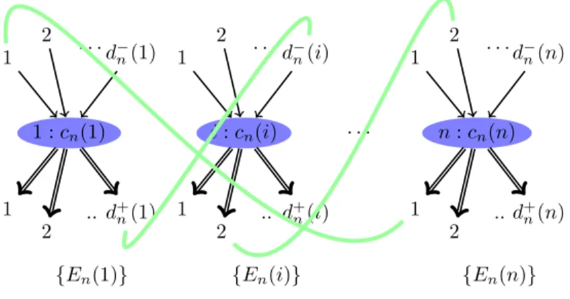
2. Structural modeling of default contagion: the network approach 19 1 : cn(1) d−n(1) · · · 2 1 d+ n(1) .. 2 1 i : cn(i) d−n(i) · · · 2 1 d+ n(i) .. 2 1 n : cn(n) d−n(n) · · · 2 1 d+ n(n) .. 2 1 · · · {En(1)} {En(i)} {En(n)}
Figure I.4: Configuration model
2.3.2 Weighted Configuration Model
(Definition 2.5 - Weighted Configuration Model). Given a set of nodes [1, . . . , n] and a degree sequence (d+
n, d−n), we associate to each node i two sets, Hn+(i) representing its
out-going half-edges and H−
n(i) representing its in-coming half-edges, with |Hn+(i)| = d+n(i) and
|H−
n(i)| = d−n(i). Let Hn+ =
S
iHn+(i) and Hn− =
S
iHn−(i). A prescribed set of weights
En(i) where |En(i)| = d+n(i) is assigned in an arbitrary order to i’s out-going half edges. A
configuration is a matching of H+
n with Hn−. To each configuration we assign a graph. When
an out-going half-edge of node i is matched with an in-coming half-edge of node j, a directed edge from i to j appears in the graph. The configuration model is the probability space in which all configurations, as defined above, have equal probability. We denote the resulting random directed multigraph by G∗
n(d−n, d+n, En), shown in Figure I.4.
2.3.3 Weighted Blanchard model
In Blanchard’s random graph model [24], one is given a prescribed degree sequence. Condition-ally on the sequence of out-degrees, an arbitrary out-going edge will be assigned to an end-node with probability proportional to the power α of the node’s out-degree. For α > 0, one obtains positive correlation between in and out-degrees.
The empirical distribution of the out-degree is assumed to converge to a power law with tail coefficient γ+:
µ+n(j) := #{i | d+n(i) = j} n→∞
20 Chapter I. Overview The main theorem in [24] states that the marginal distribution of the out-degree has a Pareto tail with exponent γ−= γ+
α , provided 1≤ α < γ
+:
µ−n(j) := #{i | d−n(i) = j} n→∞
→ µ−(j)∼ jγ−+1.
In Chapter V, we extend this model to account for the heterogeneity of weights. The intuition behind our construction can be given by rephrasing the Pareto principle: 20% of the links carry 80% of the weights. Therefore, we will distinguish between two types of links. Links of type A represent a percentage a of the total number of links, but carry a percentage a′ of
the total mark-to-market value. All other links are said to be of type B. We can now define the random graph model.
(Definition 4.3 - Weighted Blanchard Model). Let (d+
n(i))ni=1 a prescribed sequence of
out-degrees, assumed to verify Condition 4.2. For every node i, its d+
n(i) in-coming links are
partitioned into d+,A
n (i) links of type A and d+,Bn (i) links of type B:
d+n(i) = d+,An (i) + d+,Bn (i). (I.24)
We denote mA :=Pn
i=1d+,An (i) and by mB :=P n
i=1d+,Bn (i) the total number of links of type
A and type B respectively. We let FA : Rm+A → [0, 1] and FB : Rm
B
+ → [0, 1] the joint
proba-bility distributions functions for links of type A and B respectively. The probaproba-bility distribution functions FA and FB are assumed to be invariant under permutation of their arguments.
The random graph is generated then as follows:
• Generate the weighted subgraph of links of type A by Blanchard’s algorithm with prescribed degree sequence (d+,A
n (i))ni=1 and parameter α > 0.
• Draw mA random variables from the joint distribution FA. Assign these exchangeable
variables in an arbitrary order to the links of type A. • Proceed similarly for the links of type B.
3
Contributions of the thesis
We make here a chapter by chapter summary of this thesis’ contributions. Part of this overview, referring to the network approach to systemic risk, will be published as a chapter entitled
Mathematical modeling of systemic risk, Financial Networks, Springer Series in Mathematics [110].
The models introduced in Subsections 2.2.3 and 2.2.4 are an original contribution of this thesis. They are intended to provide a base, according to the author’s own view, for joint modeling of illiquidiy and insolvency cascades. We model the causal links between these types of cascades as price feedback effects.