HAL Id: hal-02330172
https://hal.archives-ouvertes.fr/hal-02330172
Submitted on 26 May 2020
HAL is a multi-disciplinary open access
archive for the deposit and dissemination of
sci-entific research documents, whether they are
pub-lished or not. The documents may come from
teaching and research institutions in France or
abroad, or from public or private research centers.
L’archive ouverte pluridisciplinaire HAL, est
destinée au dépôt et à la diffusion de documents
scientifiques de niveau recherche, publiés ou non,
émanant des établissements d’enseignement et de
recherche français ou étrangers, des laboratoires
publics ou privés.
Seismic structure across the rift valley of the
Mid-Atlantic Ridge at 23°20’ (MARK area):
Implications for crustal accretion processes at slow
spreading ridges
J. Pablo Canales, John A. Collins, Javier Escartın, Robert Detrick
To cite this version:
J. Pablo Canales, John A. Collins, Javier Escartın, Robert Detrick. Seismic structure across the rift
valley of the Mid-Atlantic Ridge at 23°20’ (MARK area): Implications for crustal accretion processes
at slow spreading ridges. Journal of Geophysical Research : Solid Earth, American Geophysical Union,
2000, 105 (B12), pp.28411-28425. �10.1029/2000jb900301�. �hal-02330172�
JOURNAL
OF
GEOPHYSICAL
RESE•CH,
VOL.
105,
NO.
B12,
PAGES
28,411-28,425,
DECEMBER
10,
2000
Seismic
structure
across
the rift valley
of the
Mid-Atlantic
Ridge
at 23020
' (MARK area)' Implications
for crustal accretion
processes
at slow
spreading
ridges
J. Pablo Canales and John A. Collins
Department of Geology and Geophysics, Woods Hole Oceanographic Institution, Woods Hole, Massachusetts
Javier
Escartin'
Instituto
de
Ciencias
de
la
Tierra,
Consejo
Superior
de
Investigaciones
Cientfficas,
Barcelona,
Spain
Robert S. DetrickDepartment
of Geology
and
Geophysics,
Woods
Hole
Oceanographic
institution,
Woods
Hole,
Massachusetts
Abstract.
The
results
from
a 53-km-long,
wide-angle
seismic
profile
across
the
rift
valley
of the
Mid-Atlantic
Ridge
south
of the
Kane
transform
(near
23ø20'N,
MARK
area)
provide
new
constraints
on
models
of tectonic
extension
and
magmatic
accretion
along
slow
spreading
mid-
ocean
ridges.
Anomalously
low
middle
and
lower-crustal
P wave
velocities
beneath
the
neovolcanic
Snake
Pit
ridge
are
consistent
with
elevated
axial
temperatures
and
with
the
presence
of
4+1%
partial
melt
evenly
distributed
within
the
lower
crust
in
preferentially
oriented,
elongated
thin
films.
If the
melt
inclusions
have
larger
aspect
ratios,
melt
fractions
can
be
up
to 17+3%.
This
and
other
geological
observations
suggest
that
the
study
area
is
presently
in a magmatically
active
period.
The
igneous
crust
is anomalously
thin
beneath
both
flanks
of the
median
valley
(<_29.3-2.5
kin).
Thus
the
mantle
rocks
observed
along
the
western
rift
valley
wall
at
Pink
Hill
were
probably
emplaced
at
shallow
levels
within
the
valley
floor
during
a period
of very
low
magma
supply
and
were
later
exposed
on
the
valley
walls
by
normal
faulting.
The
crust
within
the
eastern
rift
valley
and
flanking
rift
mountains
is seismically
heterogeneous,
with
igneous
crustal
thickness
variations
of_>2.2
km
over
horizontal
distances
of •-5
km.
This
heterogeneity
indicates
that
the
magma
supply
in
the
area
has
fluctuated
during
the
last-2
m.y.
Thus
magmatic
and
amagmatic
periods
at
slow
spreading
ridges
may
alternate
over
much
shorter
temporal
scales
that
previously
inferred
from
sea
surface
gravity
data.
1. Introduction
Seafloor-spreading
processes
along
mid-ocean
ridges
depend
on
the
thermal
structure,
magma
supply,
and
tectonic
processes
taking
place
at the
ridge
axis.
Oceanic
crust
formed
along
mid-
ocean
ridges
with
high
magma
supply,
such
as
the
fast
spreading
East
Pacific
Rise
(EPR)
or hotspot-influenced
slow
spreading
ridges
like the Reykjanes
Ridge,
is thought
to be laterally
homogeneous
and
composed
of magmatic
rocks
(basalt,
diabase,
and
gabbro).
This
interpretation
has
been
inferred
from
seafloor
observations,
gravity,
magnetics,
marine
seismic
studies,
ophiolite
studies,
and
laboratory
measurements
of both
deep-
ocean
and
ophiolite
rocks
[e.g.,
Christensen,
1978;
Salisbury
and
Christensen,
1978;
Kempnet
and
Gettrust,
1982].
This
has
led
to
the
commonly
accepted
idea
that
mature
fast
spreading
crust
is
layered
in seismic
units
that
•'eflect
lithological
and/or
porosity
changes
with
depth
[e.g.,
Vera
et al., 1990;
White
et al., 1992;
Derrick
et aI., 1994].
Now
at Laboratoire
de P6trologie,
Universit6
Pierre
et Marie
Curie/CNRS, Paris.Copyright
2000
by
the
American
Geophysical
Union.
Paper
number
2000JB900301
0148.0227/00/2000JB900301509.00
Oceanic
crust
formed
along
slow
spreading
ridges
(<50
mm/yr
full rate)
like
the
Mid-Atlantic
Ridge
(MAR)
has
a layered
seismic
structure
similar
to that
of fast
spreading
crust
[e.g.,
White
et al., 1992;
Canales
et aI., 2000].
However,
geological
observations
indicate
that
the
composition
of slow
spreading
crust
is instead
highly
heterogeneous
and/or
discontinuous
[e.g.,
8onatti,
1976;
Karson
et aI., 1987;
Cannat
eta!.,
1995b].
This
structural
variability
is attributed
to spatial
and temporal
variations
in magmatic
and
tectonic
processes
that
take
place
within
the
axial
valley
[e.g.,
Tucholke
and
Lin, 1994].
It has
been
proposed
[PockaIny
et aI., 1988]
that slow
spreading
ridges
alternate
between
periods
of reduced
magma
supply
when
tectonics becomes the major control on the structure of the ocean
crust
and
periods
of more
robust
magmatic
activity
when
crustal
accretion
processes
resemble
those
at fast spreading
ridges.
Gravity-derived
crustal
thickness
variations
at slow
spreading
crust
along
flow lines
have
been
interpreted
as an indicator
of
temporal
variations
in magma
supply.
Pariso
et al. [1995]
and
Tucholke
et al. [1997]
suggested
that
such
temporal
variations
have
a periodicity
of 2-5 m.y.,
based
on inferred
relative
crustal
thickness
variations
of_+2
km along
flow lines.
The alternation
between
magmatic
and
tectonic
periods
is
commonly
invoked
by models
that
explain
the eraplacement
of
lower
crust
and
upper
mantle
rocks
on the
seafloor
(e.g.,
see
review
by LagabrieIIe
et aI. [1998]).
One
model
suggests
that
mantle
rocks
are
emp!aced
at the seafloor
by a purely
tectonic
28,412
CANALES
ET AL.: SEISMIC
STRUCTURE
OF THE MARK AREA
process in which faulting plays the major role. Extension along low-angle faults during periods of low magma supply may unroof and expose lower crust and upper mantle rocks [e.g., Dick
et al., 1981; Karson, 1990; Mutter and Karson, 1992; Tucholke and Lin, 1994]. A variation of this tectonic model suggests that
within a magmatically active segment, crustal accretion may be
asymmetric, resulting in the transfer of most of the igneous crust
to one side of the ridge axis and the exposure of ultramafic rocks
at the conjugate side, as observed by the asymmetry of inside-
outside comers [e.g., Allerton et aI., 2000]. An alternative model
proposes a long-lived, magma-starved period during which a thin, discontinuous magmatic crust is formed by gabbroic intrusions within upper mantle peridotires [Cannat, 1993].
In this paper we present results from a seismic profile across the rift valley of the MAR near 23ø20'N. We show that the present-day axial structure is consistent with a period of
enhanced magmatism and provides important constraints on the
distribution of partial melt within the axial slow spreading crust. We also show that the seismically imaged crust on the flanks of the rift valley is anomalously thin and seismically heterogeneous, providing constraints on the mechanism of eraplacement of mantle rocks on the seafloor and on the periodicity of magmatic and tectonic phases of seafloor spreading at this slow spreading ridge.
2. Mid-Atlantic Ridge South of the Kane
TransformThe MAR south of the Kane transform (Figure 1), known as the MARK area, is one of the best studied sections of the MAR. The present full-spreading rate at this location is ~25 mm/yr, with faster rates to the west (14 mm/yr) than to the east (! 1 mrn/yr) during the last 3 m.y. [Schulz et al., 1988]. Part of this asymmetry seems to be caused by an eastward jump of the ridge axis -1.7 m.y. ago [Schulz et aI., 1988]. Off-axis geophysical studies [Genre et aI., 1995; PockaIny et al., 1995; Maia and Genre, 1998] revealed a complex tectonic pattern attributed to the rapid growth and waning of short-lived segments during the last
10 m.y. The MAR between 22ø30'N and 23ø40'N is segmented in two spreading cells separated by a discordant zone at ~23ø10'N thought to be a zero-offset discontinuity [Karson et al., 1987; Kong et aI., 1988].
The -40-km-long northern segment is highly asymmetrical, with a prominent elevated inside-comer massif at the western side of its intersection with the Kane transform [Karson and Dick, 1983] (Figure !a). The western rift valley wall is characterized by a large fault scarp that exposes gabbro and
serpentinized peridotires along the whole length of the segment
[e.g., Mdvel et al., 199!] (Figure lb) and has been the target of several Ocean Drilling Program (ODP) legs [Derrick et al., 1988; Cannat et al., 1995a]. It has been interpreted to represent the initial stage of the formation of an "oceanic core complex" similar to those found in other MAR areas [Cann et al., 1997; Tuchotke et al., 1998]. The eastern flank is characterized by smaller faults and a continuous basaltic carapace with hummocky
morphology characteristic of volcanic construction [Karson and
Dick, 1983; Karson et al., 1987; Kong et aI., !988; Smith et al., 1995].
The ~15-km-wide rift valley floor of the northern segment is characterized by a 500- to 900-m-high, 4- to 6-km-wide, 40-kin- long neovolcanic ridge (Snake Pit ridge) constructed over a highly tectonized axial valley floor [Karson et al., 1987; Karson
and
Brown,
1988;
Kong
et al., 1988;
Genre
et al., 1991]
(Figure
1). The reflective, hummocky acoustic textures that characterize the Snake Pit ridge are indicative of fresh, unsedimented basalts
[Kong
et aI., 1988],
and/or
of a thin
sediment
cover
[Genre
et al.,
1991].
Recent
dating
of basalts
from
the Snake
Pit ridge
using
2'•U
2•øTh
"'•U?Pa
and
2'•øTh-n6Ra
disequilibria
suggests
an
age
of only 10+_2 ka for the youngest lavas [Sturm et al., 2000]. The presence of a vigorous hydrothermal system at 23ø22'N [ODP
Leg 106 Scientific
Party, !986; Campbell
et al., 1988]
suggests
elevated temperatures and heat sources at shallow or midcrustallevels.
Earlier studies of basalts collected along the neovolcanic zone
showed a very homogeneous composition [Thompson et aI.,
!986], suggesting a massive eruption from one or more, well. mixed magma chambers (consistent with compositionally diverse melts feeding the lower crust that are efficiently mixed within crustal magma chambers [Coogan et al., 2000]) or successive eruptions from isolated magma chambers with a similar degree of evolution [Karson and Brown, I988]. However, a more recent
analysis of closely spaced basalt samples along the 40-kin length
of the Snake Pit ridge have revealed the existence of enriched mid-ocean ridge basalts (MORBs) near the center of the neovolcanic zone [Donnelly et al., 1999], suggesting that a
magma source may be located at the center of this spreading cell.
Despite the strong geological evidence suggesting that the northern segment is magmatically active, efforts to image a crustal magma body beneath this section of the ridge using near-
vertical incidence seismic methods have been inconclusive
[Derrick et al., 1990; Calvert, 1995, !997]. Wide-angle seismic
data suggest that the crust along the northern segment is 4-5 krn
thick with no distinctive layering, indicative of a highly tectonized lithosphere during a period of low magma supply [Purdy and Derrick, 1986]. The axial mantle Bouguer anomalies are very irregular [Morris and Derrick, 1991] and differ substantially from the typical bull' s-eye gravity low found along other MAR segments [Linet al., 1990; Derrick et aI., 1995].
3. Seismic Experiment and Data
As part of the Nobel at the Mid-Atlantic Ridge (NOMAR) Seismic Experiment (June-July !997) [Collins and Derrick,
!998], we carried out an ocean bottom seismic refraction
experiment at the MAR at 23020 ' (profile NOMAR6). Four ocean bottom hydrophones (OBH), three ocean Reftek in a ball (ORB) hydrophones, and two ocean bottom seismometers (OBS) were deployed along a 53-km-long profile across the rift valley
of the northem
segment
of the MARK area
(Figure
1). OBS
50,
and ORBs 2 and 3 were deployed in the eastern flank of the median valley; OBS 64, ORB 1, and OBH 25 on the valley floor flanking the Snake Pit ridge; and OBHs 16, 22, and 26 were
deployed
on the western
flank of the rift valley.
OBH 26 was
coincident with the location of ODP Hole 920 on the flank ofPink
Hill, and
OBH 22 was
emplaced
on the
summit
of Pink
Hill.
This configuration provided a mean spacing between instr-uments
of 4.3 kin. The instrument locations are listed in Table 1.
All of the instruments recorded seismic arrivals from 329 air
gun
shots
generated
with the R/V Maurice
Ewing's
8420
cubic
inch
(138
L), 20-air-gun
array
towed
at a depth
of--10 m. The
profile
was shot twice with different
repetition
rate: 120 s
(seismic
trace
spacing
of 252 _+
21 m), and 180 s (seismic
trace
spacing
of 395 _+
29 m). Shot
positions
were
obtained
from
he
shipboard
Global
Positioning
System
(GPS)
position,
corrected
CANALES ET AL.' SEISMIC STRUCTURE OF THE MARK AREA 28,413 a) 45' 30'W 23' 45'N • 23' 30'N 23'15'N 45' 30'W
b) 23'
45'N
23'30'N 23'15'NC) basaltic
overlavas
serpentinitesnonconformably
-• 14 rnm/•/rspruadlng
I 11rato
mm/yr • -2.5 '•OBH 22OBH 16 . • OBH 26 pillow lavas • _ "-'-r% ODP-920 / • o rr . •/'-
•' -3.0
•.
...:-:::::'.X
:::::::::-•//
young
pillowbasaltic
lavas //
\ m••
m o
o• pk ^ _ t"/NI--
'"
':'":':':" .
/., ,o o "•/
._. . ..:.:. • / • • \_c:
ß *-'-3.5
serpentinite::'"::ii;-:
-.-.z: ,-.,-
m o/
m • .:.. o o r'h -4.0 ':: - exposures in ß - 4.5 Pink Hill 4 •new crust constructed
W under Snake Ptt ridge normal faults
-•5 -•0
-•
d
•
lb
lb
2b 2•
Across-axis distance (km) -2500 -35OO -425O -6200Figure 1. (a) Bathymetry map of the northern segment of the MARK area (Mid-Atlantic Ridge south of the Kane transform). Depth contours every 250 m. Thick solid line is the seismic profile NOMAR6, with instrument locations denoted by labels in boxes. The profile crosses the neovolcanic zone (Snake Pit ridge, dash-dotted line) and the location of ODP Hole 920 at Pink Hill. Dashed lines show, approximately, magnetic anomalies redrawn from Schulz et al. [1988], Pockalny et al. [1995], and Tucholke et al. [1998]. Inset shows the central Atlantic and the location of the MARK area. Thick line is the Mid-Atlantic Ridge, and thin lines are some major fracture zones. (b) Simplified geological map of the study area. Solid line with solid dots is profile NOMAR6. Thick solid line denotes the western wall fault along which gabbros (light shaded) and serpentinites (dark shaded) m-e exposed. Open circles are the location of the several ODP drill holes in the area. Other features as the neovolcanic ridge and a detachment surface at ---45ø18'W [Tucholl, e et aI., 1998] are indicated. Gray depth contours every 500 m. (c) Bathymetry profile along NOMAR6. The simplified geological cross-section is modified from Lagabrielle et al. [1998]. Location of the instruments and ODP Hole 920 are indicated with labels. Spreading rates are fiom Schulz et al. [1988].
28,414 CANALES ET AL.: SEISMIC STRUCTURE OF THE MARK AREA
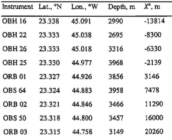
Table 1. Instrument Positions
Instrument Lat., øN Lon., øW Depth, m .,P, rn OBH 16 23.338 45.091 2990 -13814 OBH 22 23.333 45.038 2695 -8300 OBH 26 23.333 45.018 3316 -6330 OBH 25 23.330 44.977 3968 -2139 ORB 01 23.327 44.926 3856 3146 OBS 64 23.324 44.883 3958 7478 ORB 02 23.321 44.846 3466 11290 OBS 50 23.318 44.800 3457 16000 ORB 03 23.315 44.758 3149 20260
'•X is the projected position of the instruments along the profile, where the coordinate origin has been arbitrarily assigned to the cross point between the profile and the summit of the
Snake Pit ridge.
for the distance between the GPS antenna and the air gun array (88 m).
The seismic data were recorded by each instrument at 200
samples/s and reduced to the standard Society of Exploration Geophysicists (SEG-Y) format after correcting for the time drift
of the internal clock of the instrument. For plotting and
interpretation purposes, we applied a band-pass filter of 5-20 Hz to the record sections. No further data processing was required to
enhance arrivals. Most of the record sections show a high signal-
to-noise ratio (Figure 2), allowing a clear identification of the
first-arrival travel times.
Our analysis is based on first arrivals attributed to turning
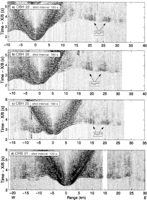
rays, without making a distinction between crustal (Pg) and mantle (Pn) arrivals. We do not observe clear crust-mantle boundary reflections (ProP) as secondary arrivals or Pg-PmP-Pn triplications in the data. In contrast we observe discontinuous, high-amplitude ProP-like first arrivals (Figure 2) that are attributed to turning rays within a high-velocity gradient zone.
We measured 2075 hand-picked travel time picks, which are
shown in Figure 3 plotted against shot-receiver distance, reduced
to 8 kmJs and corrected for the water path travel time. For a
given range, travel times can differ as much as 0.6 s, suggesting
that the seismic structure varies considerably along the profile. Also, the arrivals at offsets >20 km have an apparent velocity of 8 kin/s, indicating that mantle-type velocities are present at
shallow levels.
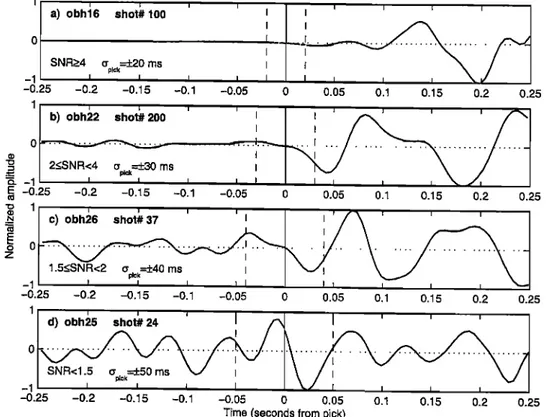
We consider two sources for the travel time uncertainties. First, errors in the shot-receiver offset (+65 m, instruments were not relocated) and in the bathymetry at the ray entry point (+20 m) introduce travel time errors of __.13 ms and +8 ms, respectively. Then we added the root-mean-sum of those errors (+15 ms, common to all the shot-receiver pairs) to the picking uncertainty that depends on the signal-to-noise ratio (SNR) of each trace. We inspected the SNR following the method of ZeIt and Forsyth [1994]. The SNR was calculated as the square root of the ratio between the trace energy in a 250-ms window before and after the pick. The relation between the SNR and the total expected travel time uncertainty is given in Table 2. In Figure 4 we show four selected traces with their travel time pick and uncertainty representative of the four cases considered in the error estimate. Since the travel time picks were identified and
selected by visually correlating adjacent traces, the uncertainty in
the noisiest traces is lower than if the picks were selected in individual traces. Furthermore, the accuracy of travel time
picking
in noisy
traces
(usually
related
to a shot
repetition
rate
of
120 s) was improved by comparing the seismic signature with
that of traces at similar offsets with higher SNR recorded with a shot repetition rate of 180 s.
4. Results
We used the tomographic method of Toomey et al. [1994] to invert P wave travel times for both the one-dimensional (i-D) and two-dimensional (2-D) seismic structure along profile NOMAR6. The slowness (i.e., velocity) model is defined on a 56-by-10-km regular grid with a nodal spacing of 100 m in both horizontal and vertical directions. The perturbation grid had a
spacing of 200 m in the vertical direction and 500 m in the
horizontal direction for the 2-D inversion. 4.1. One-Dimensional Structure
We first inverted the travel time data for the best fitting depth-
dependent 1-D velocity model. The motivation was to obtain a starting velocity model for the 2-D inversion that is representative of the average seismic structure of the area and to
be able to interpret the 2-D structure as deviations from the
regional structure. Furthermore, the 1-D inversion allows us to
investigate the resolution of the model with depth and to evaluate
the dependence of the results on the starting velocity model.
We tested two initial velocity models (Figure 5a): MAR23N,
obtained by Purdy and Derrick [1986] in this same area (south of
23ø15'N), and EPR9N, obtained by Vera et aI. [1990] in 180- kyr-old crust at the EPR. The best fitting 1-D model from EPR9N is obtained after 9 iterations, and the root-mean-square (RMS) travel time residual is reduced from 214 to 101 ms. For the MAR23N, the best solution is obtained after 4 iterations,
reducing the RMS from 275 ms to 97 ms. Figure 5a shows that both solutions are very similar from 1 to 4 km below the
seafloor. They differ within the upper 1 km, although the mean velocities are similar (3.9 and 4.0 km/s for the solutions from
EPR9N and MAR23N, respectively). This is an indication that
with our data distribution the method cannot resolve the fine-
scale structure within the first kilometer but only the average structure. Figure 5b shows that the resolution starts to decrease at 4 km below the seafloor (and probably is responsible for the
difference in velocity between 4 and 6 km depth) and that the
model cannot resolve the seismic structure for depths >6 km.
4.2. Two-Dimensional Structure
We obtained the 2-D velocity structure along profile NOMAR6 by inverting the P wave travel times allowing horizontal and vertical perturbations of the slowness model and using as a starting velocity model the best 1-D solution obtained
from MAR23N (Figure 5a). Damping and spatial smoothing
constraints need to be included in the inversion procedure to stabilize the solution. We constrained the variance of the model
parameters
to be 20% of the starting
model.
The method
of
Toomey
et aI. [ 1994]
makes
use
of a smoothing
parameter
)• and
a decay length •: that must be carefully chosen beforehand. We
inspected
several
combinations
of both parameters,
with
values
of 20, 40, 50, 100,
and
300
and
• y,..
values
of 0.5,
0.6,
0.8, 1, 1.5, and 2 km. From all of the resulting models weconsidered
as acceptable
those
models
that gave
a normalized
CANALES ET AL.' SEISMIC STRUCTURE OF THE MARK AREA 28,415
5•'
1 a) OBH
22' shot,nterval:
180s
•,•-J::•<;'z:,:,½.•½,l•?•,,.•,,::•½•½,,;;•2!!•;iI•}'•t•tti•iilr
.- •,• .' . .•'
..,,i
•.,
, ...
I- , } } ....
•
-10 -5 0 5 10 15 20 25 30 35
I-
-lO
b) OBH 26' shot interval' 180 s
-5 0 5 10 15 20 25 30
'• I t ,,I,,,.
,,..I.
t,-, . - _'.,•,•1
...
•..• ,.,
....
...-..•:•,•,...-.,,,.,
,.,,,
},•
, ill,.
t 't•-,
,'-.,
...
',,.
.*.-.,
,,,,.'•--•
,.,,,
.... :•,
,-
.rl,,l,
I,il.
-•5 -10 -5 0 5 10 15 20 25
d) ORB 01; shot •nterval. 120 s
,,:.:;.,,,• ,-.,.½.:,•._•• ,, . .... .,,,•, _.,=:;. :-.: ..,2',•,.,., •. ,. • ...,•,,o,.., , , ".,"'2":.;:: -20 -15 -10 -5 W 4O 35 40 1 30 35
ß
. ,t: ."
'• "---' ,'";..,..,.
,•, .,,,,"f.,,,
,• •...,,,,..
it.
;%%.',., ;:..':.,:'½ ... . ,.½.' .,,.,.,,,' .,,• ,I • ... ltt ,, •, . 0 5 10 15 20 25 30 Range (km) EFigure 2. Observed seismic record sections from some selected instruments. Data have been reduced to 8 km/s and band-pass filtered between 5 and 20 Hz. Amplitudes have been scaled with range using a power law gain. Three cases with shot repetition rate of 180 s are shown for (a) OBH 22; (b) OBH 26; and (c) OBH 25. Note the intermittent, high-amplitude ProP-like arrivals. (d) One example of data recorded with shot repetition rate of 120 s (ORB 1). Note the differences in trace spacing and signal-to-noise ratio.
misfit parameter Z-' of 1 between the predicted and observed
travel times. From this subset of models we then selected our best fitting final model as the one with the larger )• (the smoothest one). Thus the final velocity model (Plate l a) was obtained from an inversion with Z =100, 'r =0.6 km, and
x. y, • x. •,
'r.=0.5 km and gives a misfit parameter Z-=I with an overall RMS
residual travel time of 29 ms. The comparison between the predicted and observed travel times is shown in Figure 6.
The most prominent feature of the model is the alternating pattern of mantle-type (>_7.5 krn/s) and crustal-type (_<7.0 kin/s)
velocities between 2 and 5 km subseafioor depth across the rift
valley. The eastern and western flanks of the axial valley are both
characterized by mantle.-type velocities at shallow levels (2-4 km below the seafloor). In contrast, the axial zone (-7 km wide
centered on the Snake Pit ridge) has much lower seismic
velocities. Middle and lower crustal-type velocities (---6.5 kin/s) are not reached until 5-6 km below the seafloor in this area.
In Plate lb we show the relative variation of the final velocity structure (Plate l a) with respect to the initial 1-D velocity model obtained from MAR23N (Figure 5a). Within the uppermost kilometer of the crust, there are several positive anomalies that are spadally correlated with the footwall of several small, inward facing faults. The anomalies to the east of the Snake Pit ridge (at 8, 17.5, and 22 km model distance) have an amplitude of 0.6 krn/s, while the anomaly associated with the base of Pink Hill (6 km to the west of the Snake Pit ridge) has an amplitude of 1 km/s. Also within the uppermost crust there is a prominent negative anomaly (-1.2 krn/s) immediately to the west of the neovolcanic ridge.
28,416 CANALES ET AL.: SEISMIC STRUCTURE OF THE MARK AREA 2.0 1.5 0.0 0 10 20 30 40 Range (km)
Figure 3. Observed travel times versus shot-receiver range. Times have been corrected for a reduction velocity of 8 krn/s and for the travel time through the water column.
negative anomaly of- 1.0 to -1.4 km/s that extends down to 5-6 km below the seafloor. At depths >1.5 kin, the western rift mountains have somewhat higher seismic velocities than the
eastern flank. On both sides of the axial zone there are discrete,
3- to 5-km-wide positive anomalies with amplitude of 0.6-1.2 km/s. The transition from the axial negative anomaly to the off- axis positive anomalies is sharp and occurs in a distance of 1-2 km.
In Figure
6 we show,
for each instrument,
the ray paths
associated with the observed travel time picks, the predicted and observed travel times, and the variation of the amplitude of the seismograms with range. The amplitude-offset plots show some interesting features. For example, arrivals to the east of OBHs 22,
Table 2. Total Travel Time Pick Uncertainties
SNR a Number of Picks Error, ms SNR>4 657 +20 2<SNR<4 852 +30 1.5<SNR<2 326 +40 SNR<I.5 240 +50
•SNR is the signal-to-noise ratio (see text for details).
26, 25, and
ORB 1 show
strong
amplitudes
associated
with
rays
that primarily sample the discrete high-velocity bodies to the eastof the axial zone. This correlation suggests that the top of the
high-velocity bodies may act as a discontinuous crust-mantle
transition responsible for the intermittent, high-amplitude, PmP-
like arrivals. We cannot rule out the possibility that scattered
energy due to topography may also contribute to the high-
amplitude arrivals.
4.3. Model Uncertainty and Resolution Analysis
We estimated
the accuracy
of our results
using
the Monte
Carlo
method
[e.g.,
Zhang
et al., 1998;
Korenaga
et al., 2000].
The uncertainty
of a nonlinear
inversion
can be expressed
in
terms of the posterior model covariance matrix [e.g., Taranto!a, 1987], which can be approximated by the standard deviation of a
large
number
of Monte
Carlo
realizations
assuming
that all the
realizations
have the same
probability
[e.g., Matarese,
1993].
The uncertainty
estimated
by this
method
should
be interpreted
1 -- - I I I I
a) obhl6 shot#
100
I I '
'
'
'
'
I
-1 I I • • I -0.25 -0.2 -0.15 -0.1 -0.05 0 0.05 0.1 0.15 0.2 0.25 I 0 ... • ... ,, .... .__= E -0.25 -0.2 -0.15 -0.1 -0.05 0 0.05 0.1 0.15 0.2 0.25 • c) Obh26 shot• 37 I I ' • • o 0 ... I. Z =•40 ms1.5•SN
R<2 •pick
-1 • • • •., ,.I -0.25 -0.2 -o.s -0,05 0 0.05 o.s 0,2 0.2s J d) obh25 shotS24'
'
0 ..._1 /
,
P I
•
I
-0.25 -0.2 -0.15 -0.1 -0.05 0 0.05 0.1 0.15 0.2 0.25 Time (seconds from pick)Figure
4. Selected
seismic
traces
representative
of the
four
cases
considered
for estimating
the
pick
error
based
in
the analysis
of the signal-to-noise
ratio (SNR). Horizontal
axis is time, with 0 s corresponding
to the pick
identification
(vertical
solid
line).
The vertical
dashed
lines
represent
the total
travel
time
uncertainties
(see
Table
2
and text for details). Vertical axis is trace amplitude, normalized to the maximum value observed in the windowCANALES ET AL.: SEISMIC STRUCTURE OF THE MARK AREA 28,417 V p (km/s) Normalized DWS 2 3 4 5 6 7 8 0.0 0.2 0.4 0.6 0.8 1.0 0 0 1 1 -,- -, .... • .... r - 3 3 .c:4 4 5 5 6 6 7 7 8 8
Figure 5. (a) Starting velocity models (EPR9N thin dashed line from Vera et al. [1990] for 180-kyr-old Pacific crust, and MAR23N thins solid line from Purdy and Derrick [1986] for the study area) and their best one-dimensional solution (thick dashed
and solid lines, respectively). Note how different initial velocity models converge in similar results between 1 and 5 km depth. (b)
Resolution in depth given by the derivative weight sum (DWS) [Toomey et al., 1994].
as uncertainty for our given space model (i.e., starting velocity model and smoothing constraints). A Monte Carlo realization is computed by inverting the observed travel times (perturbed with a randomly generated noise) with a random initial velocity model. We generated 10 random initial velocity models by adding smooth perturbations randomly distributed (15 and 3 km wavelength in the horizontal and vertical direction, respectively, and maximum amplitude of +0.4 km/s) to our best fitting model (Plate l a). We also generated 10 random observation vectors following the method of Zhang and Toksi•z [1998]. This method realistically simulates the travel time errors by adding to the
observed travel times a common receiver random Gaussian
distribution N(0, o'• c ) and a random Gaussian perturbation N(0,
2 2 =10ms and
cry, ) to the travel time gradients. We used
2 .
cry, = 15 ms km -• Thus we obtained 100 Monte Carlo realizations by inverting all the combinations of the 10 initial velocity models with the 10 observation vectors, using the same model parameterization as in the final solution. With this degree
of perturbation, the initial RMS misfit was -46 ms and the
-2.8. All of the Monte Carlo inversions converged rapidly to
We show in Plate l c that the uncertainty of the calculated
velocities for most of the model is below +0.15 km/s and locally increases to about +0.25 km/s at the bottom of the model. Plate
ld shows the normalized DWS, a proxy to the ray density. We
note that the smallest uncertainty (<0.1 kin/s) is obtained at
depths shallower than -6 km, not where the ray coverage is
maximum (between 5.5 and 8 km deep). Also, the deep high-
velocity areas have the largest uncertainty (>0.2 krrds). These
results are consistent with the fact that low velocities with small
uncertainty predict travel times with the same accuracy as high
velocities with larger uncertainties.
We conducted a series of resolution tests to assess whether our
data can effectively resolve velocity anomalies of the same
amplitude and dimensions as those showed in Plate lb. We tested
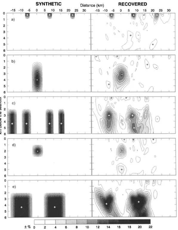
three major features: the 2- to 3-km-wide anomalies located within the upper kilometer (Figure 7a), the axial middle and lower crustal negative anomaly (Figure 7b), and the off-axis deep positive anomalies (Figure 7c). In each case we generated synthetic travel time data produced by synthetic anomalies (Figure 7, left) with maximum amplitude of +20% with respect .to our preferred 1-D solution (Figure 5a). This is based on the fact that the major anomalies of Plate lb represent deviations of _+18- 22% from the initial velocity model. We inverted the synthetic travel times (perturbed as in the Monte Carlo inversions) using the same model parameterization as in the final solution.
The recovered features (Figure 7, fight) show that all of the major velocity anomalies can be well detected with our data and instrument distribution. The dimensions of the anomalies are
well constrained, although the recovered amplitudes in all cases are somewhat lower than the initial ones. Although we showed that the recovered structure within the uppermost kilometer is strongly dependent on the starting velocity model (Figure 5a), Figure 7a shows that even small, shallow features can be well resolved with our experiment configuration if the starting velocity model is close enough to the real structure. We also tested the possibility that the deep axial negative anomaly could be an artifact produced by a negative anomaly within the middle crust smeared down in the tomography inversion. Figure 7d shows that a single --1.5-km-thick midcrustal anomaly would be detectable by our data without affecting the deeper structure. Thus, although some percentage of the axial low-velocity zone could be an artifact produced by the off-axis high-velocity anomalies (Figure 7c), the anomalously low seismic velocities beneath the Snake Pit ridge up to 6 km below the seafloor are required by the data. We also tested that the data require the discrete high-velocity bodies imaged to the east of the Snake Pit ridge. Figure 7e shows that a single, larger structure in the eastern flank would not be imaged as two individual, smaller structures due to lateral variations in the ray coverage.
5. Interpretation and Discussion
Profile NOMAR6 can be divided in two areas with distinct seismic characteristics: the ~7-km-wide axial zone centered on the Snake Pit ridge and the areas east and west of the axial zone to which we will refer as the off-axis areas.
5.1. Off-Axis Structure
On the western ridge flank the 1 km/s positive anomaly immediately beneath OBH 26 (Plate lb) is coincident with the belt of serpentinites exposed along the western rift valley wall [Karson et al., 1987], and with ODP Hole 920 [Cannat et al., 1995a]. Miller and Christensen [1997] calculated a mean V• of 5.42+0.39 km/s (at a confining pressure of 200 MPa) for the ultramafic rocks representing the 200-m-long section recovered at ODP Hole 920. Although our data cannot resolve the seismic structure at this small vertical scale (200 m), the seismic velocity within the upper 1 km beneath OBH 26 increases from 3.5 to 5.5 km/s (vertical profile extracted at X=-6.3 km, Figure 8a), similar to the measurements of Miller and Christensen [1997]. At subseafloor depths >2.5 km, the western flank is characterized by seismic velocities >7.5 km/s (Plate l a and Figure 8a), probably representing peridotitic mantle. Thus the igneous crust on the
28,418 CANALES ET AL.: SEISMIC STRUCTURE OF THE MARK AREA • Blue), o• s8o 1 BldO • HBO 9• 9 t HBO OS SBO • 8•o g•, HBO 91 HBO (tu>l) 4ldec] o o. • BNO
Og
880•
•
o
9• HBO • HBO gt HBO (tu4) q•,deaCANALES
ET AL.' SEISMIC
STRUCTURE
OF THE MARK
AREA
28,419
•.. 2.5 I ! T i ! • I ib)
OBH-22
•
,
10 •' 3.5 •_ 2.5 4 6 8 10 c) OBH-26 3.53.0
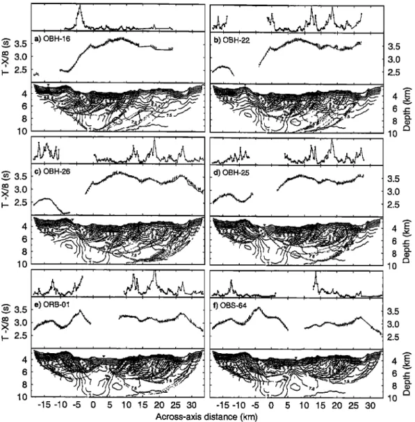
2.5 ,,-, r , i , t i i ,• ,,, f t i -15-10 -5 0 5 10 15 20 25 30 -15-10 -5 0 5 10 15 20 25 30 Across-axis distance (km) 10 3.5 3.0 2.5 3.5 3.0 2.5 3.5 3.0 2.5Figure 6. (a)-(i) For all the receivers from west to east. (bottom): Ray coverage for the model of Plate la.
Annotated contours are every 0.5 krn/s. Solid triangle denotes the position of the receiver. (middle): Observed
(vertical bars) and predicted (solid line) travel times, reduced to 8 km/s. The height of the observed travel time bars is equal to their associated uncertainty. (top): Amplitude of the seismograms versus offset. The amplitude is measured as the maximum deflection of the seismic trace in a 0.6-s window after the first-arrival travel time pick. For each instrument the amplitudes have been amplified using a gain scale law (offsee) and then normalized to the maximum value. The vertical axis represents one unit. Note that for OBHs 22, 26, 25, and ORB 1, rays primarily sampling the isolated high-velocity bodies to the east of the Snake Pit ridge correspond to strong increases on the
amplitude of the arrivals. Compare also with the observed record sections (Figure 2).
western ridge flank is at most 2.5 km thick, and it could be
thinner
if velocities
<7.5 krn/s
represent
serpentinized
peridotite.
Along the eastern valley flank,. the positive anomalies within
the
uppermost
crust
(Plate
lb) probably
reflect
variations
in the
thickness
of the extrusive
layer
(submersible
dives
and
dredges
reported mostly basaltic rocks to the east of the Snake Pit ridge
[e.g.,
Karson
et al., 1987;
Brown
and Karson,
1988],
although
these
observations
do not
extend
as far east
as our
profile).
This
across-axis variation could be produced by temporal fluctuations
in the volume
of magma
erupted
on the seafloor
and/or
by
faulting
and
exposure
along
fault scarps
of basaltic
rocks
with
lower
porosity
as
the
crust
ages.
We favor
this
later
interpretation
given
that
the anomalies
are located
at the foot of topographic
features
like
small
inward
facing
faults.
At two locations along the eastern flank (at 7 and 16 km to the east of the Snake Pit ridge, Plate l a), we obtained velocities >7.5 km/s at very shallow depths, thus constraining the igneous
crustal thickness at these locations to be <2.3 km and 3.2 km,
respectively. The other areas of the eastern flank (e.g., vertical profile extracted at X=12.4 km, Figure 8a) have a seismic structure which is similar to that observed at the rift valley of other MAR segments [Hoofi et al., 2000] and to the average structure of young Atlantic crust [White et al., 1992] (Figure 8a), with velocities increasing from 6.5 to 7.3 km/s within 2.3-4.5 km
below the seafloor. These velocities are consistent with a lower
crust primarily composed of gabbros or with serpentinized mantle. We find the later interpretation very unlikely since there is not a clear reason to explain why along the eastern flank some
28,420 (2ANALES ET AL.' SEISMIC STRUCTURE OF THE MARK AREA
--- g)
ORB-O•
• 3.5• 3.0
•.. 2.5 4 6 8 10 • 3.53.0
•.. 2.5 -15-10 -5 0 5 10 15 20 25 30 Across-axis distance (km) h) OBS-50 •-• ... i I i, , i, i.,.
-15-10 -5 0 5 10 15 20 25 30 Across-axis distance (kin)Figure 6. (continued)
3.5 3.0 2.5
lO •
sections of the mantle would be serpentinized while others would
not, given the absence of large faults or tectonic features. Thus
the seismic
structure
along
the eastern
flank
evidences
a strong
lithospheric
heterogeneity
with
igneous
crustal
thickness
varying
from <2.3 km to >4.5 km at a horizontal scale of ---5 km. This
seismic
pattern
suggests
that
the magma
budget
in the study
area
has
experienced
rapid
and
important
fluctuations
during
the last
-2 m.y.5.2. Axial Structure
The seismic structure beneath the Snake Pit ridge is clearly
anomalous. Seismic velocities to -5 km below the seafloor are
much lower than those reported by other seismic experiments in the MAR rift valley (Figure 8a) [White et al., 1992; Barclay et al., 1998; Hoofi et al., 2000; Magde et aI., 2000]. The uppermost
crust is characterized by a negative anomaly (-1.2 kin/s)
immediately to the west of the Snake Pit ridge. This anomaly can be explained by a large accumulation of high-porosity lavas [e.g.,
Wilkens et al., 1991 ] and/or slope debris at the base of the fault
scarp. Submersible dives have reported pillow flows extending ---4 km to the west of the summit of the Snake Pit ridge (near
23ø22'N) [e.g., Brown and Karson, 1988; Genre eta!., 1991]. These flows end on a 4200- to 4400-m-deep small basin at the
footwall of a major fault, where OBH 25 is located (Figure 1). It is likely that the fault acts as a barrier and the lava ponds against the fault. The mixture of lava flows and talus deposits can locally
increase the bulk porosity of the uppermost crust. Other factors such as fractures, hydrothermal circulation, and/or elevated temperatures within the upper 1.5 km may contribute to the
negative velocity anomaly, but their relative importance is
difficult to evaluate with our data.
From 2 to 5.5 km depth, the axial seismic velocities increase from 5.5 to 6.5 km/s. These velocities are consistent with
serpentinized peridotite [e.g., Miller and Christensen, 1997] or
with a gabbroic lower crust with reduced velocities due to cracks, elevated temperatures, and/or partial melt. Several factors make the first alternative unlikely. Numerous normal faults and cracks
within the median valley could allow the penetration of fluids up to 6 km below the seafloor [e.g., Toomey et aI., 1988], altering
the axial mantle. However, since the seismic structure off-axis at
similar depths is that of unaltered mantle, this hypothesis seems unlikely. Alternatively, a single major fault could act as the path for fluids reaching such depths. The fault along the western valley wall is the most likely candidate, but it would have to extend across the rift valley up to 5 km to the east of the Snake
Pit ridge
to explain
the extent
of the axial
low-velocity
zone.
Two observations
make
this
hypothesis
also
unlikely.
First,
the
seismic
velocities
suggest
that
the serpentinization
front
does
not
penetrate
below
2.5 km beneath
the western
valley
wall. Second,
the fluid compositions
and temperatures
of the Snake
Pit
hydrothermal
vent
field
suggest
a maximum
depth
of the
reaction
zone of 2 km below the seafloor
[Campbell
et al., 1988].
Furthermore,
it is unlikely
that the fluid pressure
exceeds
the
lithostatic
pressure
at 6 km below the seafloor,
as would
be
required
to serpentinize
the axial mantle
by fluid penetration
along
opened
and
connected
fractures
at such
depths.
Lithostatic
pressure
and
ductile
flow are likely to close
pores
and small cracks at depths >2 kin. Thus the low seismic
velocities
within
the lower
crust
beneath
the Snake
Pit ridge
are
most
likely
produced
by elevated
temperatures
and
the presence
of partial
melt.
In order
to estimate
the fraction
of partial
melt
required
to explain
those
velocities,
we compare
the axial
velocity
structure
(vertical
profile
extracted
at X=0 km, Figure
8a) with the off-axis structure that resembles that of normalyoung Atlantic crust (vertical profile extracted at X=12.4 km).
Thus we are assuming that the seismic structure of the axial zone
will resemble
that
observed
at -12 km east
of the Snake
Pit ridge
once the crust ages and cools, and the melt is extracted. AnCANALES ET AL.: SEISMIC STRUCTURE OF THE MARK AREA 28 421 -15 -10 -5 I 4- 5- 6 • 0 i 1- b) 2- 3 4 5 - 6 •
SYNTHETIC
Distance
(kin)
0 5 10 15 20 25 30 ß I I I i t i I RECOVERED -15 -10 -5 0 5 10 15 20 25 30 I I
E)
I I - % 0 2 4 6 8 10 12 14 16 18 20 22Figure
7. Resolution
tests.
(left):
Synthetic
velocity
anomalies
and
(right)
the recovered
features.
Contours
are
every
+2%
of velocity
perturbation.
(a) Positive
anomalies
within
the
uppermost
kilometer.
(b) Deep
axial
low-
velocity
zone.
(c) Discrete
off-axis
high-velocity
bodies.
(d) Midcrustal
axial
low-velocity
zone.
(d) Large
ofl"-axis
high-velocity bodies. See text for details.
alternative hypothesis is that the axial zone is upper mantle with
reduced velocities due to temperature and melt. In such a case, the seismic structure once the crust ages would resemble that observed at X=7 km or X=-6.3 km (Figure 8a). We do not
explore this hypothesis since it seems inconsistent that the large
melt fraction that would be required to explain the large velocity differences between X=0 km zmd X=-6.3 km would produce such a thin igneous crust (<2.5 kin).
We first calculate the fraction of the velocity difference between X=0 km and X=12.4 km that can be explained by
elevated temperatures, and then we interpret the thermal- corrected velocity anomaly in terms of partial melt. As a thermal
reference model we use the near-axis thermal structure obtained
by Henstock et al. [1993, Figure 7g] for a slow spreading rate. We assume an anharmonic dependence of V,, with temperature
(T) in the form
of 3V•,I•T =-0.57x10 -• kms
'• K -! , as calculated
for MAR gabbros by Christensen [1979]. We also assume that the axial temperatures cannot exceed the liquidus temperatureTt.(øC)=191MgO(wt %)+1054 [Sintm• and Derrick, 1992].
![Figure 5. (a) Starting velocity models (EPR9N thin dashed line from Vera et al. [1990] for 180-kyr-old Pacific crust, and MAR23N thins solid line from Purdy and Derrick [1986] for the study area) and their best one-dimensional solution (thick d](https://thumb-eu.123doks.com/thumbv2/123doknet/2354234.37101/8.909.88.445.84.411/figure-starting-velocity-models-pacific-derrick-dimensional-solution.webp)