UNIVERSITÉ DE MONTRÉAL
POWER-EFFICIENT HARDWARE ARCHITECTURE FOR
COMPUTING SPLIT-RADIX FFT ON HIGHLY SPARSE SPECTRUM
HANIEH ABDOLLAHIFAKHR
DÉPARTEMENT DE GÉNIE ÉLECTRIQUE ÉCOLE POLYTECHNIQUE DE MONTRÉAL
MÉMOIRE PRÉSENTÉ EN VUE DE L‟OBTENTION DU DIPLÔME DE MAÎTRISE ÈS SCIENCES APPLIQUÉES
(GÉNIE ÉLECTRIQUE) AOÛT 2015
UNIVERSITÉ DE MONTRÉAL
ÉCOLE POLYTECHNIQUE DE MONTRÉAL
Ce mémoire intitulé :
POWER-EFFICIENT HARDWARE ARCHITECTURE FOR COMPUTING SPLIT-RADIX FFT ON HIGHLY SPARSE SPECTRUM
présenté par : ABDOLLAHIFAKHR HANIEH
en vue de l‟obtention du diplôme de : Maîtrise ès sciences appliquées a été dûment accepté par le jury d‟examen constitué de :
M. DAVID Jean-Pierre, Ph. D., président
M. SAVARIA Yvon, Ph. D., membre directeur de recherche
M. GAGNON François, Ph. D., membre et codirecteur de recherche M. LANGLOIS Pierre, Ph. D., membre
DEDICATION
To My beloved, Jaber To My Lovely Mother, Malihe To My Patient and Sympathetic Father, Mahmoud And to My Kind Brother, Hamon
ACKNOWLEDGEMENTS
I would like to express my sincere gratitude to professors Yvon Savaria and François Gagnon and to Normand Bélanger for all their support, patience, generosity and advices during my master‟s studies in Polytechnique Montréal.
RÉSUMÉ
Le problème du transfert des signaux du domaine temporel au domaine fréquentiel d'une manière efficace, lorsque le contenu du spectre de fréquences a une faible densité, est le sujet de cette thèse. La technique bien connue de la transformée de Fourier rapide (FFT) est l'algorithme de traitement de signal privilégié pour observer le contenu fréquentiel des signaux entrants à des émetteurs-récepteurs de télécommunication, tels que la radio cognitive, ou la radio définie par logiciel qu‟on utilise habituellement pour l‟analyse du spectre dans une bande de fréquences. Cela peut représenter un lourd fardeau de calcul sur des processeurs lorsque la FFT ordinaire est mise en œuvre, ce qui peut impliquer une consommation d'énergie considérable. L'alimentation en énergie est une ressource limitée dans les appareils mobiles et, par conséquent, cette ressource peut être critique pour des dispositifs de télécommunications mobiles.
Dans le but de développer un processeur économe en énergie pour les applications de transformation temps-fréquence, un algorithme de transformée de Fourier plus efficace, en termes du nombre de multiplications et d‟additions complexes, est sélectionné. En effet, la Split-Radix Fast Fourier Transform (SRFFT) offre une performance meilleure que la FFT classique en termes de réduction du nombre de multiplications complexes nécessaires et elle peut donc conduire à une consommation d'énergie réduite.
En appliquent le concept d‟élagage des calculs inutiles, c‟est-à-dire des multiplications complexes avec entrées ou sorties à zéro, tout au long de l'algorithme, on peut réduire la consommation d'énergie.
Ainsi, une architecture matérielle énergétiquement efficace est développée pour le calcul de la SRFFT. Cette architecture est basée sur l'élagage des calculs inutiles. En fait, pour tirer parti du potentiel de la SRFFT, une nouvelle architecture d'un processeur de SRFFT configurable est d'abord conçue, puis l'architecture est développée afin d‟éliminer les calculs inutiles. Cela se fait par l‟utilisation appropriée d'une matrice d'élagage. Le processeur proposé peut trouver des applications dans le multiplexage orthogonal en fréquence (OFDM) dans des émetteurs-récepteurs de communication, où les signaux transmis peuvent n‟occuper qu'une petite partie de
l'ensemble du spectre opérationnel. Le processeur est mis en œuvre sur un circuit programmable (FPGA) et sa fonctionnalité ainsi que sa performance sont validées par des simulations.
En outre, la consommation de puissance des processeurs SRFFT avec ou sans moteur d‟élagage est analysée via le simulateur de puissance du simulateur. Prenant le processeur SRFFT sans élagage comme référence, les simulations de consommation d'énergie montrent que l'économie d'énergie maximale obtenue est de l'ordre de 20% lors de l'élagage d‟une FFT de 1024 points appliquée à des signaux de spectre très clairsemé.
ABSTRACT
The problem of transferring a time domain signal into the frequency domain in an efficient manner, when the frequency contents are sparsely distributed, is the research topic covered in this thesis. The well-known Fast Fourier Transform (FFT) is the most common signal processing algorithm for observing the frequency contents of incoming signals in telecommunication transceivers. It is notably used in cognitive or software defined radio which usually demands for monitoring the spectrum in a wide frequency band. This may imply a heavy computation burden on processors when the ordinary FFT algorithm is implemented, and hence yield considerable power consumption. Power and energy supply is a limited resource in mobile devices and therefore, efficient execution of the Fourier transform has turned out to be critical for mobile telecommunication devices.
With the purpose of developing a power-efficient processor for time-frequency transformation, the most computationally efficient Fourier transform algorithm is selected among the existing Fourier transform algorithms upon studying them in terms of required arithmetic operations, i.e. complex multiplications and additions. Indeed, the Split-Radix Fast Fourier Transform (SRFFT) offers a performance that is better than conventional FFT in terms of reduced number of complex multiplications and hence, can reduce power consumption.
Appling the concept of pruning of the unnecessary computations, i.e. complex multiplications with either zero inputs or outputs, throughout the whole algorithm may reduce the power consumption even further.
Thus, a power efficient hardware architecture implementing the SRFFT is developed through pruning unnecessary computations. In fact, leveraging the potential in SRFFT algorithm, a new architecture of a configurable SRFFT processor is first devised and then the architecture is developed further so that unnecessary computations, which yield zeros at the output, are pruned. This is done through stalling butterfly computations with appropriate use of a pruning matrix. The proposed processor may find applications in orthogonal frequency division multiplexing (OFDM) communication transceivers, where transmitted signals may occupy only a small
portion of the whole operational spectrum. The processor is implemented on a field-programmable gate array (FPGA) and its performance is validated via simulations.
In addition, the power consumption analysis of the SRFFT processors with and without the pruning engine is performed using a power analysis simulation tool.
Taking the SRFFT processor without pruning engine as a reference, the power consumption simulations show that a maximum power saving of around 20% is achieved when the pruning engine outputs are actively used in to the SRFFT processor computing the 1024-point Fourier Transform of signals with a very sparse spectrum.
TABLE OF CONTENTS
DEDICATION……….. III ACKNOWLEDGMENTS……….IV RESUME………V ABSTRACT………..VII TABLE OF CONTENTS………..IX LIST OF TABLES…….………..XI LIST OF FIGURES…….……….XII ABREVIATIONS……….…...XV CHAPTER 1 INTRODUCTION ... 11.1 Background and motivation ... 1
CHAPTER 2 PREVIOUS CONTRIBUTIONS ON FAST FOURIER TRANSFORM PRUNING ………..3
CHAPTER 3 APPLICATION OF FFT IN WIRELESS COMMUNICATION TRANSCEIVERS ………...………...………..………..8 3.1 OFDM transceivers ... 8 3.2 FFT formats ... 11 3.2.1 Radix-2 FFT ... 11 3.2.2 Radix-4 FFT algorithm ... 14 3.2.3 Split Radix FFT (SRFFT) ... 17 3.3 Pruning ... 18
3.4 The most efficient FFT algorithm ... 20
3.5 Software implementation and analysis of FFT and pruned FFT ... 22
CHAPTER 4 STUDY AND DEVELOPMENT OF POWER EFFICIENT SRFFT PROCESSOR ... 26
4.1 Implementation of SRFFT processor ... 26
4.1.1 Architecture of the proposed SRFFT processor ... 26
4.1.2 L-shaped butterflies ... 26
4.1.3 Control unit ... 28
4.1.4 RAMs and interconnects ... 31
4.1.5 Twiddle factor ROM ... 35
4.2 Butterfly engine structure ... 36
4.2.1 Simulation results... 40
4.3 SRFFT pruning ... 43
4.3.1 Matrix pruning generation ... 46
4.4 Simulations ... 52
4.5 Synthesis and assessment of power consumption ... 57
4.5.1 Discussion………..58
CHAPTER 5 CONCLUSIONS AND FUTURE WORK ... 59
REFRENCE………...………60
LIST OF TABLES
Table 2-1: Total number of complex multiplications in different FFT structures [25, 37] ... 6
Table 4-1: Examples of bit configuration of twiddle factor ... 36
Table 4-2: The result of the 8-point SRFFT ... 40
Table 4-3: Comparison between Matlab with proposed SRFFT ... 42
Table 4-4: Results of pruned SRFFT computations ... 55
Table 4-5: Comparison of the computed results ... 56
LIST OF FIGURES
Figure 2-1: Total number of complex multiplications in different FFT architectures [25] ... 7
Figure 3-1: General NC-OFDM Transceiver Architecture [16] ... 10
Figure 3-2: Decimation in frequency of a length-N DFT into two length- DFTs preceded by a preprocessing stage [30]. ... 13
Figure 3-3: The butterfly, a basic DIF computation unit ... 14
Figure 3-4: Radix4 decimation in frequency FFT butterfly [31] ... 16
Figure 3-5:FFT in DIF structure with ordinary implementation ... 19
Figure 3-6: Representation of a single “butterfly”; the twiddle factors are defined by . ... 19
Figure 3-7: FFT pruning scheme proposed by Markel ... 20
Figure 3-8: The data flow FFT pruning architecture ... 21
Figure 3-9: Input signal ... 23
Figure 3-10: Result computed with the implemented software FFT ... 23
Figure 3-11: The input signal used to test the iFFT; 25% of the carriers are non-zero ... 24
Figure 3-12: Comparison of the number of operations required, i.e. summations and multiplications, for a 256-point FFT computed using different algorithms ... 25
Figure 4-1: Architecture of the proposed SRFFT ... 27
Figure 4-2: L shape butterfly ... 27
Figure 4-3: Butterfly engine ... 28
Figure 4-4: 16-point SRFFT and processing progress [33] ... 29
Figure 4-5: Addresses generated while computing an 8 point SRFFT ... 30
Figure 4-6: Addresses generated while processing a 16 point SRFFT ... 31
( /16) exp( 2 /16)
k
Figure 4-7: The architecture of pipeline SRFFT ... 32
Figure 4-8: Address and control signals at the output of FSM block ... 33
Figure 4-9: Reading 4 data points from RAM and sorting them at the input of butterfly engine 34 Figure 4-10: Writing the results into RAMs ... 35
Figure 4-11: Twiddle factor binary word configuration ... 36
Figure 4-12: Pipelined butterfly 1 and 2 ... 37
Figure 4-13: Pipelined butterfly 3 ... 39
Figure 4-14: The modified butterfly engine ... 40
Figure 4-15: Input of the SRFFT ... 41
Figure 4-16: Results of the SRFFT ... 41
Figure 4-17: Inputs of the 16 point SRFFT ... 43
Figure 4-18: Outputs of the 16 point SRFFT ... 43
Figure 4-19: 8 point SRFFT diagram... 44
Figure 4-20: Pruning matrix of 16 point SRFFT with a typical data input ... 46
Figure 4-21: Pruning matrix of the 8 point SRFFT with two non-zero values at the output; ... 49
Figure 4-22: The modified SRFFT architecture with pruning engine ... 50
Figure 4-23: Structure used for controlling the butterflies ... 51
Figure 4-24: Structure used for butterfly stalling ... 51
Figure 4-25: 16-point SRFFT pruning; matrix pruning generation for a typical last column input, Part I ... 52
Figure 4-26: 16-point SRFFT pruning; matrix pruning generation for a typical last column input- Part II ... 53
Figure 4-28:Results of the computation ... 54 Figure 4-29: Split radix pruning with 16-point inputs ... 55 Figure 4-30: Results of a 16 point SRFFT with pruning ... 56
LIST OF SYMBOLS AND ABBREVIATIONS
FFT Fast Fourier TransformSRFFT Split Radix Fast Fourier Transform
OFDM Orthogonal Frequency Division Multiplexing
LIST OF APPENDICES
Appendix A SRFFT SYNTHESIS REPORT ... 64
Appendix B SRFFT PLACE & ROUTE REPORT ... 66
Appendix C SRFFT PRUNING SYNTHESIS REPORT ... 68
Appendix D SRFFT PRUNING PLACE & ROUTE REPORT ... 72
Appendix E POWER REPORT FOR SRFFT WITHOUT PRUNING ENGINE FOR 1024 ... 74
Appendix F POWER REPORT WITH PRUNING FOR 1024 NON-ZERO ... 78
Appendix G FOR VALIDATING THE SRFFT PERFORMANCE ... 81
CHAPTER 1
INTRODUCTION
1.1
Background and motivation
Along with the increasing demand for radio technology related services, the issue of developing techniques for utilizing available radio-frequency bands optimally is currently an important research topic. Furthermore, the techniques are being developed with the purpose of preventing interferences, which may reduce the data throughput and channel reliability in wireless networks [1, 2, 3, 4].
On the other hand, the licensed part of the radio spectrum is often poorly used and therefore practical means must be developed to improve spectrum utilization. Therefore, a growing attention has been given to configurable and multi-standard radios [5, 6]. Software defined radios (SDRs) that integrate various radio architectures in the back-end for different standards [5] or cognitive radios (CRs) that can reconfigure the architecture and optimize the operational parameters in a reconfigurable manner [6] are good examples of the recent developments in this regard.
Spectrum sensing plays an important role nowadays in several wireless communication techniques such as backhaul small cell communication [7] or CR systems [4]. Cognitive radio is explored as a means to improve wireless communications and it could become a reliable solution to the spectrum underutilization problem. Furthermore, the ultimate objective of CR systems is to provide highly reliable and available communication means between all users and to also facilitate more efficient utilization of the radio spectrum. CRs are actually able to sense the spectrum in the environment and recognize unused frequency bands so that they can make best use of available resources. In CR, several unused frequency bands could be located in different segments of some reserved spectrum. Furthermore, spectrum allocation can be done while preventing interference with other frequency bands that are actively used. This technique is called spectrum pooling [8].
Theoretically, an orthogonal frequency division multiplexing OFDM-based Cognitive Radio system can optimally approach the Shannon capacity in the segmented spectrum using adaptive resource allocation on each subcarrier.
In these OFDM transceivers, the radio frequency (RF) signals may not include all subcarriers, implying that the transceivers in cognitive radio devices try to remain aware of the spectrum segments that are used and unused. A common technique for spectrum sensing is Digital Signal Processing (DSP), specifically the Fast Fourier Transform (FFT) algorithm. Indeed, OFDM transmits a large number of narrowband carriers, closely spaced in the frequency domain. In order to avoid a large number of modulators and filters at the transmitter and complementary filters and demodulators at the receiver, it is desirable to be able to use modern digital signal processing techniques, such as the FFT. Thus, one consequence of maintaining orthogonality is that the OFDM signal can be defined using Fourier transform procedures. But, the FFT of the operational signal may yield many zero-valued frequency bins or bins that are “Don‟t Cares” for some applications. This means that a processor performing those calculations may carry out many unnecessary computations, which increase power consumption. Considering that mobile devices must minimize power consumption in order to ensure that the batteries of those devices will power the device for a sufficiently long period of time on a single charge, our goal is to propose means to minimize the number of computations performed.
The rest of this thesis is organized as follows. In Chapter 2, the reported research in this area is reviewed with the purpose of contextualizing this thesis work. Subsequently, efficient fast Fourier transform algorithms are studied and compared in order to develop the most appropriate algorithm to be applied to sparse spectrum in Chapter 3. Then, the architecture of the proposed FFT processor is explained in detail in the following Chapter 4. Also, the pruning engine which is added on purpose is presented and finally, the overall power consumption of the proposed FFT core with and without the pruning engine is compared through power simulation analysis upon implementation on FPGA. A power savings on the order of around 20% is concluded in Chapter 5.
CHAPTER 2
PREVIOUS CONTRIBUTIONS ON FAST FOURIER
TRANSFORM PRUNING
The considerable demand for computationally efficient FFT algorithms and processors in wireless technology, in particular for NC-OFDM transceivers, has driven a research in this direction [12, 17]. Furthermore, developing FFT algorithms with minimum number of computations when a significant number of zeros exist in either the input or the output of the FFT has been subjected to intensive research [13-25]. Reconfigurable algorithms that can adapt to the conditions at the input or output may be used to reduce power consumption. Because means of effectively computing the Fourier transform may find applications in today‟s mobile wireless communication devices, development and implementation of power efficient FFT cores have come highly relevant. In this chapter, the papers that are the basis of the current research in this area are categorized and briefly explained in order to contextualize this thesis work.
Except for work by [12] on the development of low-power FFT architectures, which was achieved through optimization of an FFT core, the majority of the published research was pursuing a specific direction, i.e. omitting unnecessary computations. This concept, which is termed “pruning”, has been introduced to eliminate useless computations [13-17]. The idea of pruning was first suggested in [13] with the purpose of increasing the computational efficiency for the decimation-in-frequency (DIF) structured FFT performed on signals whose number of non-zeros is considerably less than the length of the FFT. The main objective was to increase the computational efficiency by decreasing the total number of arithmetic operations. The technique is proposed with the purpose of reducing the computation time. Indeed, all computational operations that yield zeros are not carried out.
A very similar algorithm was developed [14] for computing the FFT of a decimated-in-time (DIT) signal. Like the pruning algorithm proposed by Markel, this allowed reducing the overall processing time. However, Skinner‟s pruning algorithm for DIT achieves a better reduction factor on the total number of multiplications. The major limitation of Markel‟s or Skinner‟s pruning algorithms is that they can only compute a contiguous series of output starting from the first one.
Therefore, a pruning technique was proposed that can prune an FFT according to zeros at either the input or output stages [19, 20]. Moreover, two efficient algorithms were proposed for simultaneous DIT and DIF, in [19] and [20] respectively. As a matter of fact, these methods combine Markel‟s pruning method to the output of Skinner‟s algorithm.
Another pruning technique was proposed [15] by which a matrix could be established in order to determine whether a specific computation must be conducted or not. Furthermore, depending on where pruning is to be implemented (i.e. at input or output), two different matrices of size are formed to specify which computations are useful. Input and output pruning matrices are obtained from the first and last column of the FFT computation diagram, respectively. In the pruning matrix, the non-zero terms at both input and output vectors are denoted by unity and the rest of the matrix is obtained from these vectors as the first or last column from the input or output pruning matrices, respectively. The main contribution of this algorithm is that the number of non-zero inputs or non-zero outputs as well as their location can be arbitrary. It also works equally well for both DIT and DIF architectures.
In [16], a pruning algorithm is proposed, which is mostly built upon previous algorithms. A considerable reduction in computation time was reported by employing the proposed matrix. It is claimed that the algorithm can efficiently and quickly prune the FFT for NC-OFDM transceivers. Contrary to the general FFT pruning proposed by [15], it avoids using conditional terms and therefore brings a considerable reduction in computation time. Unlike previous work, the size of the pruning matrix proposed by [16] for an N-point FFT is ⁄ , which is half of the size reported in [15].
The main drawback of existing pruning algorithms is their high resources utilization, i.e. data memory for storage of the configuration matrix. In [17], FFT pruning for NC-OFDM transceivers is considered again with the purpose of reducing its inevitable resource requirements when implemented. Partial pruning allows the pruning of the input until a given depth in the FFT structure, which yields a reduction in memory requirements. Moreover, through partial pruning, a compromise is made between the computational time saved through pruning and the required size of the memory for data storage. Through the developed partial pruning algorithm, a time saving close to the full pruning algorithms was achieved after implementation while 20% less
memory was required in comparison to previously reported algorithms [15, 16]. This made the algorithm more suitable for embedded-system applications with limited memory resources. In [21], a pruning algorithm called input-zero-traced FFT pruning (IZTFFTP) was proposed. It is based on the Cooley-Tukey radix-2 FFT algorithm for the applications in NC-OFDM transceiver, where the number of non-zeros outnumbers the number of zeros at either the input or the output. Through C++ simulations, the performance of the algorithm was compared with the non-pruned FFT and the reduction in the overall arithmetic operations was reported in a table. For example, 5120 complex multiplication in ordinary 1024 point FFT was reduced down to 2448 with the proposed pruned FFT with the same length. Throughout comparison of the execution time of operation of the proposed pruned FFT with the ordinary FFT, it was concluded that the computational complexity was reduced considerably.
In [13, 22], Sorensen et al. proposed an efficient algorithm called transform decomposition. Transform decomposition can be seen as a modified Cooley-Tukey FFT where the DFT is decomposed into two smaller DFTs. Transform decomposition is more efficient and flexible than FFT pruning when it is applied on the SRFFT algorithm but it is less efficient when applied on the FFT algorithm. Note that no work was found in the literature about pruning the transform decomposition.
Qiwei Zhang et al. developed a computationally efficient IFFT/FFT for OFDM-based cognitive radio on a reconfigurable architecture [23]. The proposed algorithm was based on transform decomposition [24].
As already mentioned, the fundamental strategy to reduce both overall computational time and power is to perform as few multiplications as possible. Hence, the FFT algorithm with minimum number of arithmetic operations should be the optimum algorithm for hardware implementations. Therefore, the theoretical total number of required complex multiplications in different FFT formats is compared in Table 2-1, and the values are plotted in Figure 2-1 for an easier comparison for a typical 1024-point FFT. One can observe that, among several FFT formats, including the radix-2 and the split-radix (SR), the latter requires the smallest number of multiplications and additions. Also, different formats of FFT pruning techniques are compared in accordance with the equations provided in Table 2-1. The superior performance of SRFFT
pruning in comparison to transform decomposition can be observed in Figure 2-1. Note that, unlike the Radix-2 diagram with in-place computation, the computations in the SRFFT are not carried out stage by stage, but its L-shaped butterfly advances with computations stage by stage at only its top half, while combining all computations of two subsequent stages at once in its lower half, much as in a radix-4 implementation [24]. Therefore, SRFFT is a promising form of FFT formulation, assuming the objective is to reduce power consumption with pruning.
Table 2-1: Total number of complex multiplications in different FFT structures [25, 37] N is the length of FFT, L is the number of non-zeros and
FFT Algorithms Complex Multiplication
Radix-2 FFT N/2×log2(N)
SRFFT N/3×log2(N)-8/9×(N-1)
Markel‟s FFT pruning N/2×log2(L)+N-L
Skinner‟s FFT pruning N/2×log2(L)+N-L
Transform Decomposition Based on radix-2 N/2×log2(P)+L×(N/P-1)
Based on SRFFT N/3×log2(P)-8/9×N×(1-1/P)+L×(N/P-1)
SRFFT pruning Continuous L N/18×(1/L+6×log2(L)-1)-L+1
Where L<N, L is power of 4 Arbitrary L L/N×(N/3×log2(N)-8/9×(N-1))
Figure 2-1: Total number of complex multiplications in different FFT architectures [25]
In [17], an FFT core architecture is described. It comprises a pruning engine that helps reducing the power consumption. Their FFT core was implemented on a Field Programmable Gate Array (FPGA) and a saving of 10% in power consumption due to the pruning engine was reported. In [25], a binary pruning matrix similar to the one proposed in [15] for output pruning is applied to 64-point SRFFT architecture. However, no analysis is provided on power consumption and resource utilization.
In this research work, a new architecture of a SRFFT core is developed that includes a pruning engine with the purpose of reducing power consumption. The combination of SRFFT with pruning has already been introduced. However, it has never been studied and analyzed for possible reduction in power consumption. Therefore, to the best of our knowledge, a power efficient SRFFT core with a pruning engine is developed and analyzed for the first time in this research.
CHAPTER 3
APPLICATION OF FFT IN WIRELESS
COMMUNICATION TRANSCEIVERS
In order to highlight the importance of power efficient FFT processor for OFDM-based wireless communication transceiver in the CR platform, a brief review of its fundamental architecture and operational principles is presented in this chapter. Subsequently, the FFT algorithm in its various formats including Radix-2, Radix-4 and SR-FFT is introduced. Finally, a study of pruning techniques is presented.
3.1
OFDM transceivers
As was already mentioned, spectrum sensing is the task of autonomous monitoring of the spectrum resources or sensing the radio spectrum in the local neighbourhood of the radio system. Thereby, spectrum holes or rather specifically those sub-bands of the radio spectrum that are underutilized at a particular instant of time and specific geographic location, may be detected and used efficiently. This may make more bandwidth available and consequently increase data throughput. A common part in many proposed techniques is the feature of real-time spectrum sensing or differently termed, spectrum sniffing. This allows finding available frequency bands and opportunistically use these bands for signals to be communicated in a fair and cost-effective manner. Spectrum sensing may be conducted through digital signal processing (DSP) [1, 2], radio meters [9] or, more recently, analog signal processing (ASP) [10, 11].
Through DSP techniques, the received analog signals are converted to the digital domain using analog-to-digital converters (ADCs) and then further processed to transform them into the frequency domain to obtain their power spectral density (PSD). Fast Fourier Transform (FFT) is one of the most common algorithms for obtaining the PSD of the signals.
Although DSP suffers fundamental drawbacks such as high-cost ADCs, high power consumption and poor performance at high frequencies, emphasis has recently been placed on further developments in this area. One important direction of research has been to reduce the computational burden and hence the DSP power consumption, especially for mobile devices with limited power sources.
ASP addresses some of the aforementioned challenges and is considered to be a reliable technique for signal processing at millimeter-wave frequencies for the near future [10]. However, renewed interest in ASP is recent and it still needs improvements to be a viable solution.
Nevertheless, FFT and IFFT are widely applied through digital signal processing algorithms in many communication transceivers, because, in essence, the modulation or demodulation techniques, applied to them, are based on the Fourier transform. For instance, orthogonal frequency division multiplexing (OFDM), in particular the non-contiguous OFDM (NC-OFDM), is a technology of this kind, through which modulated subcarriers may be distributed non-uniformly so that maximum bandwidth might be used for data communication. Thus, NC-OFDM is a viable transmission technology for cognitive radio transceivers operating in Dynamic Spectrum Access (DSA) networks.
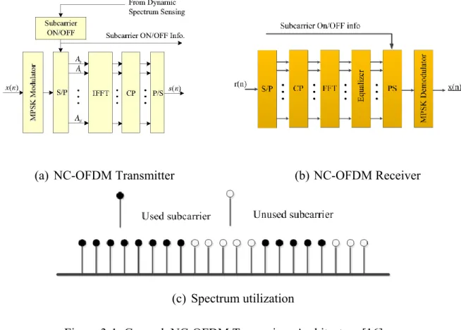
As shown in Figure 3-1, in communication transceivers with OFDM modulation, the FFT and IFFT are fundamental blocks in receiver (Rx) and transmitter (Tx) modules, respectively. Furthermore, symbols are first computed using one of the desired modulation formats, i.e. quadrature amplitude modulation (QAM) or phase shift keying (PSK), and then the modulated data stream is split into N slower data streams using a serial-to-parallel (S/P) converter. Modulation basically happens via the IFFT of these symbols when they are mapped onto several subcarriers. Thus, each OFDM symbol contains all subcarriers, each carrying modulated symbol. In order to prevent inter-symbol interference (ISI), a few fixed subcarriers are located in the beginning of the OFDM symbols using cyclic prefix (CP) blocks. The subcarriers that transmit the modulated symbols are then summed through a parallel to serial (P/S) block and transmitted upon up-conversion to the Radio Frequency (RF) range [35].
On the other hand, in the Tx module, the incoming RF signal is first down converted to baseband and then sampled and converted to digital signal through analog to digital converters. Subsequently, the OFDM symbols are de-modulated through FFT and the symbols detected using an FFT of the received signal. NC-OFDM is a special format of OFDM modulation in which the subcarriers of the OFDM symbol may be used arbitrarily and in a non-contiguous shape.
Figure 3-1 shows the architecture of the NC-OFDM transceiver along with the spectrum utilization. The architecture remains the same as that of an OFDM transceiver, which is explained above, but the subcarrier utilization would be different. Indeed, some subcarriers may be nullified in the NC-OFDM transmitter in accordance with used or unused spectrum frequency bands. This information is obtained via spectrum sensing block in Tx and is applied when data symbols are mapped on subcarriers. Users in a CR network may determine their operational frequency bands in a frequency agile and non-contiguous manner. Furthermore, in NC-OFDM, all subcarriers do not need to be active as in OFDM system, and indeed active subcarriers are located in unoccupied bands.
The information about occupied spectrum can be sent over the channel to the Rx. This information about the shape of occupied band may be used in Rx for pruning the FFT algorithm throughout demodulation and hence allow avoiding demodulation of zero subcarriers. Typical non-contiguous spectrum utilization is shown in Figure 3-1 (b).
(a) NC-OFDM Transmitter (b) NC-OFDM Receiver
(c) Spectrum utilization
3.2
FFT formats
3.2.1 Radix-2 FFT
The radix-2 decimation-in-frequency (DIF) and decimation-in-time (DIT) FFT formats are the simplest FFT algorithms that basically compute the discrete Fourier transform (DFT) [30]:
where .
The DIF radix-2 FFT computation is indeed a recursive combination of two distinct partitions of the DFT computation, which can each be computed by shorter-length DFTs of different combinations of input samples. The samples (X (k)) are separated into even-indexed (k = [0, 2, 4,…,N - 2]) and odd-indexed (k = [1,3,5,…,N-1]) outputs.
Considering only even indexed samples, we can reformulate the related part of the algorithm as follows:
(3.2)
which is basically the point DFT of .
2 1 ( ) 1 0 0
( )
( )
( )
i nk N N nk N N n nx k
x n e
x n W
1 2 0 1 1 2 2 2 ( ) 2 2 0 0 1 1 2 2 2 2 0 0 1 2 0 2 X(2 ) ( ( ) W ) X(2 ) ( ( ) W ) ( ( ) ) 2 X(2 ) ( ( ) W ) ( ( ) W )(1) 2 X(2 ) (( ( ) ( )) W ) 2 N rn N n N N N r n rn N N n n N N rn rn N N n n N rn N n r x n N r x n x n N r x n x n N r x n x nw
(3.1)For the odd termed samples we have
(3.3)
which is basically the point DFT of .
The mathematical simplifications in (3.2) and (3.3) reveal that both the even-indexed and odd-indexed frequency outputs X(k) can each be computed by a length-N/2 DFT. The inputs to these DFTs are sum or subtraction of the first and second halves of the input signal, respectively, where the input to the short DFT producing the odd-indexed frequencies is multiplied by a so-called twiddle factor terms . This is called decimation in frequency because the frequency samples are computed separately in alternating groups, and a radix-2 algorithm because there are two groups. Figure 3-2 graphically illustrates this form of the DFT computation. This conversion of the full DFT into a series of shorter DFTs with a simple pre-processing step gives the decimation-in-frequency FFT its computational savings.
1 (2 1) 0 1 2 (2 1) 2 0 1 2 0 2 (2 1) ( ( ) W ) (2 1) (( ( ) ( )) ) 2 (2 1) ((( ( ) ( )) W ) W ) 2 N r n N n N N r n N N n N n rn N N n X r x n N X r x n W x n W N X r x n x n
Figure 3-2: Decimation in frequency of a length-N DFT into two length- ⁄ DFTs preceded by a preprocessing stage [30].
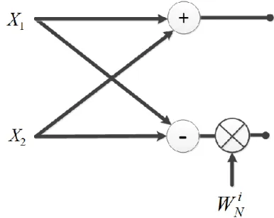
The butterfly operation is illustrated in Figure 3-3, which is basically the main computation block in the FFT. Each butterfly includes a complex addition and subtraction followed by one twiddle-factor multiplication by on the lower output branch. There are N/2 butterflies per stage. It is worthwhile to note that the length-2 FFT is just one butterfly block where the twiddle factor is 1.
Figure 3-3: The butterfly, a basic DIF computation unit
3.2.2 Radix-4 FFT algorithm
The butterfly of a radix-4 algorithm consists of four inputs and four outputs. The FFT length is , where M is the number of stages. A stage has half the number of butterflies of a radix-2 FFT stage. The radix4 DIF FFT divides an Npoint discrete Fourier transform (DFT) into four N/4 -point DFTs, then into 16 N/16--point DFTs, and so on. In the radix-2 DIF FFT, the DFT equation is expressed as the sum of two calculations: one for the first half and one for the second half of the input sequence. Similarly, the radix-4 DIF FFT expresses the DFT equation as four summations and then divides it into four equations, each of which computes every fourth output sample. The following equations illustrate radix-4 decimation in frequency [31].
(3.4)
The three twiddle factor coefficients can be expressed as follows:
Equation (3.4) can thus be expressed as
1 0 2 3 1 1 1 1 4 4 4 2 3 0 4 4 4 1 1 1 1 3 4 4 ( ) 4 ( ) 4 ( ) 4 2 4 0 0 0 0 ( ) ( ) W ( ) ( ) ( ) ( ) ( ) 3 ( ) ( ) ( ) ( ) ( ) 4 2 4 ( ) N nk N n N N N N nk nk nk nk N N N N N N N n n n n N N N N N N N n k n k n k nk N N N N n n n n X k x n X k x n W x n W x n W x n W N N N X k x n W x n W x n W x n W X k
1 4 (n ) (n ) ( ) 4 2 2 0 3 [ ( ) ( ) w ( ) w ( ) ] (1) 4 2 4 N N N N K n K nk N N N N n N N N x n x n x n x n W W
WN( N 4) K = [cos(p 2) - j sin( p 2)] K = (- j)k WN( N 2) K = [cos(p) - j sin(p)]K = (-1)k WN( N 4) K = [cos(p 2) - j sin( p 2)] K = (- j)k WN( 3N 4 ) K = [cos(3p 2 ) - jsin( 3p 2 )] k= jk 1 4 0 3 ( ) [x(n) ( ) x(n ) ( 1) ( ) ( ) ( )] (2) 4 2 4 N k k k nk N n N N N X k j x n j x n W
(3.5) (3.6) (3.7) (3.8) (3.9)To arrive at a four-point DFT decomposition, let . Equation (3.9) can then be written as four N/4 point DFTs, or
(3.10)
For k= 0 to N/4 -1.
, , and are ⁄ point DFTs. Each of the their ⁄ points is a sum of four input samples , , and , each multiplied by either 1, -1, j or –j. The sum is multiplied by a twiddle factor ( ). The four N/4 point DFTs is divided into four ⁄ -point DFT. Then, each of these N/16 point DFT is further divided into four N/64-point DFTs, and so on, until the final decimation produces four-point DFTs. The four-point DFT equation makes up the butterfly calculation of the radix-4 FFT. A radix-4 butterfly is shown graphically in Figure 3-4.
Figure 3-4: Radix4 decimation in frequency FFT butterfly [31]
1 4 0 4 1 4 0 4 1 4 2 0 4 4 0 3 (4 ) [x(n) x(n ) ( ) ( )] (3) 4 2 4 3 (4 1) [x(n) x(n ) ( ) ( )]W W (4) 4 2 4 3 (4 2) [x(n) x(n ) ( ) ( )]W W (5) 4 2 4 (4 3) [x(n) jx(n ) 4 N nk N n N n nk N N n N n nk N N n N n N N N X k x n x n W N N N X k j x n jx n N N N X k x n x n N X k
1 3 4 3 ( ) ( )]W W (6) 2 4 n nk N N N N x n jx n
3.2.3 Split radix FFT (SRFFT)
SRFFT was first introduced by Duhmel et al [27] and further developed by the same authors who presented an implementation [28]. The algorithm originates basically from the radix-2 algorithm diagram which is transformed quite straightforwardly into a radix-4 algorithm by changing the exponents of the twiddle factors. When doing so, it can be observed that a radix-4 is best for the odd terms of the DFT, while radix-2 is best for the even terms of the DFT in each stage of the diagram. Therefore, restricting the above-mentioned transformation locally to only the lower part of the diagram might improve the algorithm. This leads to a decomposition of the DFT into
(3.11)
We can see that the fundamental N-point DFT equation is decomposed into one length-N/2 DFT and two length-N/4 DFTs with twiddle factors.
The first stage of a split-radix decimation in frequency decomposition then replaces a DFT of length N by one DFT of length N/2 and two DFTs of length N/4 at the cost of [(N/2) - 4] general complex multiplications (3 real multiplications + 3 additions), and 2 multiplications by the eighth root of unity (2 real multiplications + 2 additions). The N-point DFT is then obtained by successive use of such decompositions up to the last stage, where some usual radix-2 butterflies (without twiddle factors) are needed.
The implementation of the algorithm is considerably simplified by noting that at each stage i of the algorithm, the butterflies are always applied in a repetitive manner to blocks of length ⁄ . Then, only one test is needed to decide whether the butterflies are applied to the block or not ( tests are needed at each stage i).
/2 1 2 0 1 4 3 4 0 1 4 4 0 [ ( ) ( )] 2 3 (4 3) {[ ( ) ( )] [ ( ) ( )]} 2 4 4 3 (4 1) ( {[ ( ) ( )] [ ( ) ( )]} 4 ) 2 4 2 N nk N n N n nk N N n N n nk N N n N x n x n x n N N N x k x n x n j x n x n N N N x k x n x n j x n x x k n
w
w w
w w
2iSome specific features SRFFT are listed and discussed in [27]. Within this thesis framework, the most interesting advantage of split radix FFT in comparison to other existing FFT techniques is the lowest number of required multiplications and additions.
3.3
Pruning
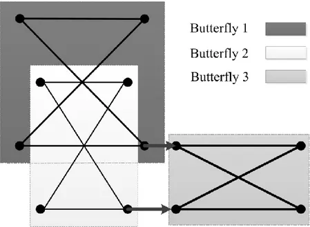
The primary pruning technique, proposed by [13], which is already introduced in Chapter 2 with the literature review, is briefly explained hereafter to provide insight on its principles.
From Figure 3-5, it can be seen that there are 4 stages, 8 butterflies per stage and 3 operations per butterfly. The structure of a butterfly computation is depicted in Figure 3-6. In general, within the diagram of an M-stage FFT, N/2 butterflies are present in each stage and each butterfly includes 3 complex arithmetic operations; i.e. one addition, one subtraction, and one multiplication.
Figure 3-7 shows a 16-point FFT with the DIF structure where the input contains only two non-zeros. Comparing the FFT with the same structure but in a un-pruned implementation, one can observe that only the computational operations originating from these two non-zero inputs that yield non-zero values in every stage were computed.
Figure 3-5:FFT computed according to the DIF structure (no pruning) [13]
Figure 3-6: Representation of a single “butterfly”; the twiddle factors are defined by .
( /16) exp( 2 /16)
k
Figure 3-7: FFT pruning scheme proposed by Markel [13]
Figure 3-7 shows pruning in the FFT through which operations that do not contribute to the outputs are eliminated. Hence, only the data paths that affect the result at the output are kept. In fact, it shows graphically a pruned 16-point FFT where only two nonzero input points are present and all arithmetic operations originating from or yielding zero values are omitted. In this diagram, we can see that pruning is possible in only three stages and pruning in the last stage is not feasible.
Since there are nonzero data points and zero value points, L=1 corresponds to the number of stages in which nothing can be pruned and M-L=3 corresponds to the number of stages in which pruning can be applied. More specifically, L is equal to the number of stages in which no pruning is allowable and thus M-L is equal to the number of stages in which pruning can be employed [13]. The implementation procedure uses careful inner-loop nesting. In essence, the algorithm is nothing more than a clever nesting of loops to provide proper indexing for the butterfly calculations.
3.4
The efficient FFT algorithm
Among the reported FFT pruning algorithms, the one proposed by Ranjbanshi et al [16] was proven to have superior performance in terms of the total processing time due to a lower number of arithmetic operations when a large number of data points at the input are zero. Moreover, the
proposed algorithm works for any pattern of zeroes at the input. Such algorithm can be used in the FFT or IFFT blocks in the NC-OFDM transceivers where a significant number of subcarriers remain null and the spectrum is sparsely utilized. Indeed, for highly sparse spectrum, the number of zero-valued inputs is quite large, and therefore considerable processing time can be saved through pruning the FFT algorithm. Therefore, the performance of this algorithm is studied as a possible candidate of further development for power saving purposes. The principles of this pruning algorithm are briefly explained next.
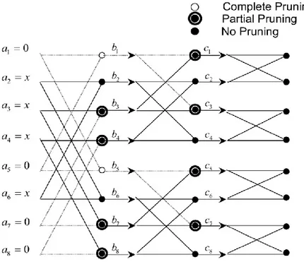
Figure 3-8 shows the developed data flow FFT pruning architecture proposed by Ranjbanshi.
Figure 3-8: The data flow FFT pruning architecture [16]
In this 8-point FFT diagram, inputs with zero and non-zero value are denoted by 0 and x, respectively. In computing the butterflies, if both inputs are zero, they will be completely pruned. If one of the inputs is non-zero the corresponding butterfly is partially pruned while the whole computation in the corresponding node would be carried out if none of the data inputs were null.
3.5
Software implementation and analysis of FFT and pruned FFT
In order to count and monitor the arithmetic operations throughout several FFT algorithms, we have implemented them with the C programming language. As a reference point, the ordinary FFT proposed by Cooley and Tukey [29] as well as the FFT pruning algorithm proposed by Ranjbanshi [16] were analyzed and implemented in C using Eclipse Helios [36].For code validation, a combination of single frequency sinusoidal signals, which are sampled with an appropriate sampling frequency, is used as input signals. The sampled input test signal is a single frequency signal oscillating at frequency and denoted by:
[ ]
Where is the sampling period and is the inverse of sampling frequency, i.e. .
At the output of the FFT with [ ] input data, a peak appears at the index which corresponds to the frequency content of the input signal, sampled at , through
(3.13)
The sampling frequency should be selected in a way that respects the Nyquist sampling period or more specifically speaking it should be at least twice as large as the largest frequency in the spectrum of the input signal.
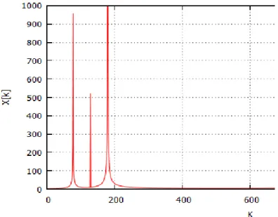
In order to validate the correctness of the programmed algorithms, a typical signal composed of three sinusoidal functions at three distinct frequencies is used as in:
[ ] (3.14) where , , . [ ], which has a sampling frequency of 4 KHz, is plotted in Figure 3-9.
Figure 3-9: Input signal
The output signal, which is in the frequency domain, is plotted in Figure 3-10. This frequency domain plot shows the existence of three peaks that correspond to three frequency components.
Figure 3-10: Result computed with the implemented software FFT
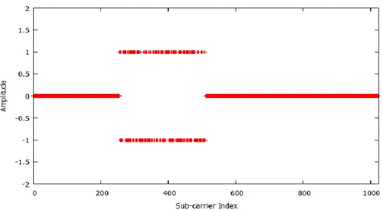
In another test, the IFFT pruning code is assessed using a data input that is the frequency components or the subcarriers of the transmitting signal of an OFDM transmitter. This set of subcarriers is selected so that three quarter of them are null, i.e. the sparseness factor is 75%. As shown in Figure 3-11,the subcarriers within the range of 256 to 511 are active, and the rest are zeros.
Figure 3-11: The input signal used to test the IFFT; 25% of the carriers are non-zero In order to compare the total number of multiplications required in the ordinary FFT (as originally proposed by Cooley and Tukey) with those required by the SRFFT, the number of multiplications and summations with various implementations of a 256-point FFT was profiled and the results are shown in Figure 3-12. One can observe that the number of multiplications and summations with the SRFFT is much less than that required with the Cooley-Tukey FFT when not using any pruning technique.
Figure 3-12: Comparison of the number of operations required, i.e. summations and multiplications, for a 256-point FFT computed using different algorithms
As one may anticipate, the SRFFT with pruning requires fewer operations than others and hence it can complete the transform process within a shorter time. Obviously, if this algorithm was implemented in FPGA, it could consume much less power. Thus, SRFFT pruning, which theoretically completes the frequency transform with minimum arithmetic operations, was selected for hardware implementation. First, an implementation of the SRFFT processor targeting an FPGA was developed and then improved for minimizing the overall power consumption by adding the pruning engine. The architecture of this processor is explained in further details in the next chapter.
100 101 102 0 200 400 600 800 1000 1200 Number of non-zeros N um be r of c om pl ex m ul tip lic at io ns SRFFT Pruning FFT Pruning Radix-2 FFT SRFFT
CHAPTER 4
STUDY AND DEVELOPMENT OF A POWER
EFFICIENT SRFFT PROCESSOR
SRFFT, which was proven to have less computation burden in comparison to other FFT algorithms, was selected for implementation in combination with the pruning technique. Therefore, a SRFFT processor is first developed and then a pruning engine is added with the purpose of increasing savings. In this chapter, the SRFFT processor as well as the pruning engine are explained in detail along with presenting the simulation results as a proof of their correct functionality. At the end, the performance of the processor with or without the pruning engine is assessed in terms of power consumption.
4.1
Implementation of SRFFT processor
4.1.1 Architecture of the proposed SRFFT processor
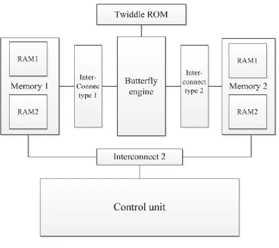
Figure 4-1 shows the architecture of the generic SRFFT processor proposed in this thesis. This processor comprises a finite state machine (FSM) as a control unit, a butterfly engine, two pairs of RAMs with single address ports for real and imaginary components of the signal, a ROM for storing the twiddle factors and several interconnect units. The functions of each block are explained further in the following.
4.1.2 L-shaped butterflies
The main difference between FFT and SRFFT is the shape of butterflies and the number of butterflies that are calculated in each stage. In Radix-2 FFT in VHDL, only one butterfly with 2 inputs is calculated while in SRFFT, 2 butterflies with 4 inputs and 1 butterfly with 2 inputs at the following stage are calculated in each round. Secondly, in the first two butterflies, we do not have multiplications with twiddle factors and thirdly, twiddle factors are arranged differently. The structure of the resulting L-shaped butterfly is sketched in Figure 4-2.
Figure 4-1: Architecture of the proposed SRFFT
Figure 4-2: L shape butterfly
Furthermore, in SRFFT, a combination of Radix-2 and Radix-4 index mapping is used for even and odd indexed data in each stage, respectively. This decomposition yields arithmetic
computations grouped in L-shape butterflies. Indeed, unlike the ordinary FFT in which computations are carried out stage by stage, those in SRFFT involve two adjacent stages. This adds to the complexity of control-signal generation and design. Figure 4-2 shows a typical L-shaped butterfly needed in the SRFFT. This butterfly can be decomposed into three distinct blocks, and in our proposed architecture, each of these blocks carry out a portion of the computations as highlighted in Figure 4-3.
Figure 4-3: Butterfly engine
4.1.3 Control unit
Figure 4-4 shows the diagram of a 16-point SRFFT and the forward flow of processing from the input stage until the output stage. Each L-shape section may contain at least one L-shape butterfly. The computation diagram of an N-point SRFFT contains -1 L-shaped stages and one ordinary or non-L-shaped stage in the last one. In this diagram, one can see three L-shaped stages, which are numbered and may contain several L-shaped butterflies.
In the proposed architecture of the SRFFT processor, a control unit, which is a finite state machine, is used to accomplish several main tasks, including 1) address generation, 2) control of
data and address paths, and 3) assignment of read and write operations for the RAMs at the appropriate time.
Figure 4-5 shows the simulation results of the initial architecture of the SRFFT processor. The addresses generated for calling the data points from RAM for an 8 point SRFFT can be observed on the signals i0, i1, i2 and i3. Also, the signal “Kport” shows the forward progress in L-shaped stages. There are two L-shape butterflies in the first stage, i.e. the first two, while there is only 1 shaped butterfly in the second stage. Furthermore, when the signal varies from 1 to 3. Two L-shape butterflies with index values 1, 3, 5, 7 and 2, 4, 6, 8 take part in the first stage when “Kport” is 1. In the second stage, when “Kport” is 2, one L-shape butterfly operates with index values 1,2,3,4, and finally in the last stage, two ordinary butterflies with index values 5, 6 and 7, 8 are carried out. In addition, address management to produce twiddle factors for 16 point SRFFT are shown in Figure 4-6. For each L-shape butterfly, two complex twiddle factors are sent to the multipliers in the butterfly units. Real and imaginary components with 16-bit-long twiddle factors are called “Wr1”, “Wr2”, “Wi1” and “Wi2” respectively.
Figure 4-6: Addresses generated while processing a 16 point SRFFT
4.1.4 RAMs and interconnects
The SRFFT processor comprises two pairs of RAMs, which contain 16-bit words, taken from two memory blocks. They allow reading and writing the signal data in each stage. With the proposed butterfly engine, the conventional “ping-pong” style swapping between the RAMs for writing and reading the signals in each stage should not be employed in the usual manner, because all four outputs of the butterfly engine do not pertain to a single stage. For instance, the output of butterfly-3 in Figure 4-3 belongs to the second stage and in the proposed architecture, they must be
rewritten in the same RAM from which the four input data of the butterfly engine were called. The L-shape butterfly requires four data points to appear at its input ports simultaneously. Therefore, four addresses should be generated in the control unit for reading four data words from memory. However, the RAMs that are employed in the memory units possess only one address port, which makes the concurrent reading of four data words unfeasible. The use of single port RAMs is done on purpose, which allows avoiding complex logic and making use of block RAMs in the FPGA. Hence, the data words should be read one by one and then rearranged so that they appear at the butterfly engine all at once. It should be mentioned that use of RAMs with four
address and input-output ports would of course be a better solution if they existed as block RAMs in FPGAs on which the processor is to be implemented.
Figure 4-7 shows the address and data word management at the input and output of a memory. In the control unit, four address words are generated and then pipelined to appear at the address port of the RAM upon being multiplexed onto a single path. Then, the data words at the output of the RAM are de-multiplexed onto four separate signal paths and then pipelined to appear in parallel at the butterfly blocks. A similar structure is also used for writing the result of computations (by the butterfly engine) back into the memory. Thereby, single-address port memory blocks are used in order to reduce the complexity and area usage.
Figure 4-7: The architecture of pipeline SRFFT
As the data would appear at the output of the RAM with one clock cycle delay, these control signals should last for 2 clock periods. The data that goes through the block “Datapipe” will appear at the input of each butterfly at the same time.
Figure 4-8 shows the behaviour of interconnect control signals, which control the parallel-to-serial or parallel-to-serial-to-parallel units. These control signals have four states and therefore accept values 0, 1, 2 and 3.
Active low write-enable (we) and active-high Ram-Enable (en) signals handle read/write functions of the RAMs. There is one of each signal for each RAM (i.e. we1, en1, we2 and en2). Writing takes place before changing the addresses while the reading happens four clock-cycles after changes in addresses at the output of the FSM. The signals I0, I1, I2 and I3 are connected to the address pins of the control unit. More specifically, “Spipectrl” and “Spipedata” vary from 0
to 3 in order to map the appropriate signals at the address port of the RAM. The signal “Spipedata” helps mapping the data at the output of the RAM to the input ports of the butterfly. Both signals change simultaneously when the relevant enable signal (en) and write/read signal (wr) at any specific stage are active. The signal “SpipeResctrl” helps mapping the computation results onto the input port of the RAM where the computation results are to be written. The signal “Spipectrl” remaps the addresses again onto the address port.
Figure 4-8: Address and control signals at the output of FSM block
Figure 4-9 shows a snapshot of a simulation of the SRFFT when 4 data-points are read out of the RAM and then sorted so that they appear all in parallel at the input ports of butterfly engine, simultaneously. The four address signals addi0, addi1, addi2 and addi3 are generated at the same time by the control unit. Since the addresses appear at the port one by one, we had to keep it active as long as the four addresses are passing. The signal “adi” is connected to the address ports of both RAMS. We can see that after 4 clock cycles from the time of generation of new set of addresses, they appear on “adi” consecutively. The control signal of the multiplexer that switches the addresses on “adi” is named as “SAddCtrl”, which varies from 0 to 3 and, each time, it maps one address on the data path connected to the address port of the RAMs.
At the time the first address appears at the address port of the RAMs, one pair of signals from the RAM-enable signals “Sen1”, “Sen2” and the write-enable signals “Swe1” and “Swe2” are activated simultaneously, so that the data are read out of the desired RAM. Note that the reading and writing control signal are active-high for both RAMs.
As already mentioned, the data should be located at the input ports of the butterfly blocks at the same time, and this is actually made through de-multiplexing. Indeed, the control signal of “SDataCtrl” switches the data at the output of the RAMs and sorts them at four data paths in parallel.
Figure 4-9: Reading 4 data points from RAM and sorting them at the input of butterfly engine Figure 4-10 shows the procedure through which the results of the butterfly engine are written to RAM. The butterfly blocks compute the results at different clock ticks, which makes data management complicated. This problem is resolved by appropriate pipelining at their outputs upon computations. Thereby, the computation results appear at the output port of the butterfly engine, i.e. “Outbut1x0”, “Outbut2x1”, “Outbut3x2”, “Outbut3x3”, consecutively. Then, they are sorted in series on the data path of the input port of the RAM, i.e. “XinRam1” and “XinRam2”, where the computation results should be stored. In fact, the control signal of “SResCtrl” which controls a de-multiplexer changes from 0 to 3 and thereby the computation results from butterfly engine are sorted in series on the input data port of both RAMs. In Figure 4-10, the computation results at the output of butterfly engine are highlighted with an inclined ellipse. It should be mentioned that the addresses are regenerated and then synchronized with the computation results when they arrive at the input data port of the RAM. These changes are synchronized with the changes of the regenerated addresses on the input address port. During this data writing time, the write-enable signals are deactivated, while both RAM-enable signals,
namely “Sen1” and “Sen2”, are activated. Thus, the computation results are written in both RAMs.
Figure 4-10: Writing the results into RAMs
4.1.5 Twiddle factor ROM
In all FFT architectures, multiplications take part at some fixed points with external parameters called twiddle factors. Depending on the size of the FFT or SRFFT, the number of twiddle factors and their value at each stage may vary. Usually, two different techniques are applied for generating and using the twiddle factors in FFT cores, i.e. twiddle factor bank or computing them during the FFT computations using a complex constant multiplication scheme [12] .
In order to reduce the power consumption, the first approach is used in our SRFFT core. Therefore, a bank of twiddle factors is built up. That bank can be used for generic N-point SRFFT covering from 8 to 1024 points.
Twiddle factors are complex numbers with a magnitude less or equal than unity. The size of the twiddle factor words chosen is 16 bits where the two most significant bits are assigned to sign and non-fractional value and the other 14 bits are assigned to fractional values. Figure 4-11 shows the bit configuration of the twiddle factors.
Figure 4-11: Twiddle factor binary word configuration
Table 4-1shows examples of twiddle factors converted to binary and hexadecimal numbers. Table 4-1: Examples of bit configuration of twiddle factor
Decimal Binary Hexadecimal
0.707 00.10110101000001 X"2D41"
1 01.00000000000000 X"4000"
-1 11.00000000000000 X"C000"
-0.707 11.01001010111111 X"D2BF"
4.2
Butterfly engine structure
The arithmetic operations within the butterfly 1 and 2 in the butterfly engine shown in Figure 4-12 can be expressed by the following equations, given the four inputs of D1, D2, D3
and D4: (4.1) (4.2) (4.3) In butterfly 1: (4.4) (4.5) (Imaginary) (4.6) (4.7)
(Imaginary) In butterfly 2: (4.8) (4.9) (Imaginary) (4.10) (4.11) (Imaginary) (4.12)
These equations are implemented with the structure shown in Figure 4-12. The architecture of both butterflies 1 and 2 are identical.
Figure 4-12: Pipelined butterfly 1 and 2
The results of the first and second butterflies are used as input data for further processing within butterfly 3 through the following equations.
(Real part at Index=I3), which includes the operation of “multiplication by j”
(4.13)
- (Imaginary part) at Index=I2)
(4.14)
(Imaginary part at Index=I3)
(4.15)
(Real part at Index=I2)
(4.16)
The implementation architecture of this butterfly is shown in Figure 4-13.
In the flow graph of the SRFFT, as it is shown in Figure 4-4 for length of 16 points, some frequency bins in the final stage are not part of the L-shape butterflies and they must be computed using conventional butterfly engines typically found in ordinary FFT hardware implementation. Therefore, the L-shape butterflies are stalled through gating when the computation reaches the last stage of the flow graph of our proposed SRFFT core. This allows reducing power consumption. These changes in the data path are depicted in Figure 4-14 where the final configuration of all butterfly blocks is depicted. We can see that the data flow throughout the butterfly blocks are managed using multiplexers and the computations at the final stage within the ordinary configuration of butterflies are carried out in the block “Butt Last”.
Figure 4-14: The modified butterfly engine
4.2.1 Simulation results
In order to validate the performance of the SRFFT processor, simulations were carried out and the output was compared with the FFT function in Matlab [32]. Three tests were done for SRFFT of sizes 8, 16 and 32. The input values used for the 8-point SRFFT were: 60, 23, 45, 90, 89, 87, 22, and 65. The excellent agreement between Matlab and VHDL simulation results reported in Table 4-2 shows the correct functionality of the developed SRFFT processing engine. The small observed differences in the results are easily explained by the differences in accuracy of the floating representation used in Matlab versus the 16 bit fixed point representation used in VHDL.
Table 4-2: The result of the 8-point SRFFT
Results / Index X1 X5 X3 X7 X2 X6 X4 X8
Matlab/ Real 481 -49 82 82 -91.9 33.93 33.93 -91
Matlab/Imaginary 0 0 45 -45 4.5 -50 50.5 -4.5
VHDL/ Real 481 -49 82 82 -92 34 33 -91
Figure 4-15: Input of the SRFFT
Figure 4-16: The result of the SRFFT
To validate the 16-point SRFFT, the inputs were: 200, 400, 600, 700, 800, 0, 400, 200, 100, 700, 600, 400, 300, 0, and 600. Again the results reported in Table 4-3 from our VHDL SRFFT processor operating with 16-bit words are in excellent agreement with the results from Matlab carried out on a PC in floating point. The outputs of the FFT in Table 4-3 are not sorted and are actually presented in the same order that appears in the last column of SRFFT computation diagram.
![Figure 2-1: Total number of complex multiplications in different FFT architectures [25]](https://thumb-eu.123doks.com/thumbv2/123doknet/2322311.29352/23.918.201.743.137.570/figure-total-number-complex-multiplications-different-fft-architectures.webp)
![Figure 3-2: Decimation in frequency of a length-N DFT into two length- ⁄ DFTs preceded by a preprocessing stage [30]](https://thumb-eu.123doks.com/thumbv2/123doknet/2322311.29352/29.918.176.726.158.586/figure-decimation-frequency-length-length-dfts-preceded-preprocessing.webp)