Report on Calculation of Jacobian Matrix of Poincaré Return Map for Self-synchronized 3D Walking Gaits

HAL Id: hal-01818860

https://hal.archives-ouvertes.fr/hal-01818860

Submitted on 19 Jun 2018

HAL is a multi-disciplinary open access

archive for the deposit and dissemination of

sci-entific research documents, whether they are

pub-lished or not. The documents may come from

teaching and research institutions in France or

abroad, or from public or private research centers.

L’archive ouverte pluridisciplinaire HAL, est

destinée au dépôt et à la diffusion de documents

scientifiques de niveau recherche, publiés ou non,

émanant des établissements d’enseignement et de

recherche français ou étrangers, des laboratoires

publics ou privés.

Report on Calculation of Jacobian Matrix of Poincaré

Return Map for Self-synchronized 3D Walking Gaits

Qiuyue Luo, Anne Kalouguine, Christine Chevallereau, Yannick Aoustin,

Victor de Leon Gomez

To cite this version:

Qiuyue Luo, Anne Kalouguine, Christine Chevallereau, Yannick Aoustin, Victor de Leon Gomez.

Report on Calculation of Jacobian Matrix of Poincaré Return Map for Self-synchronized 3D Walking

Gaits. [Research Report] LABORATOIRE DES SCIENCES DU NUMÉRIQUE DE NANTES. 2018.

�hal-01818860�

Report on Calculation of Jacobian Matrix of Poincaré Return Map for

Self-synchronized 3D Walking Gaits

Qiuyue Luo

, Victor De-León-Gómez

, Anne Kalouguine

, Christine Chevallereau

, and Yannick Aoustin

Fig. 1: A simplified model of a 3D biped robot. Each leg is massless and has variable length. At the contact point, the stance leg rotates passively around axes x and y, the rotation around axis z is not considered since this rotation is usually inhibited by friction in normal biped locomotion. The swing leg has a fully actuated spherical joint with respect to the concentrated mass of the hip.

I. INTRODUCTION A. Modeling of walking via LIP model

For simplification, the 3D linear inverted (3D LIP) model is used in this paper to analyze the dynamics of a humanoid robot. In this paper, the robot is approximated as a point mass with point feet and a CoM trajectory that is constrained to a horizontal plane for 3D walking.

In Fig.1, a simplified model of a 3D biped robot is illustrated. The lines connecting the two feet to the CoM are regarded as the two legs of the simplified model. The stance leg is free to rotate about axes x and y at the ground contact and the length of each leg can be modified through actuation, allowing a desired vertical motion of the pendulum to be obtained.

The configuration of the robot is defined via the position of the CoM (xm; ym; zm) with respect to the reference frame

attached to the stance foot and the position of the swing foot denoted by (xs; ys; zs). In order to explore simultaneously

the synchronization and stability of periodic orbits for many step length and width, a dimensionless dynamic model of the pendulum will be used. The normalized scaling factors applied along axes x and y depend on the desired step length S and desired step width D. Thus, a new set of viariables is defined:(X, Y, z, Xs, Ys, zs) = (x_Sm,y_Dm, zm,x_Ss,y_Ds, zs).

For a pendulum with a constant height of CoM z = zm,

the motions in the sagittal and frontal planes are decoupled. Thus, the equations of motion of the 3D LIP with respect to

the reference frame attached to the stance foot are [1]: ¨

X = ω2_X

¨

Y = ω2_Y (1)

where ω =q_zg

m characterizes the LIP and varies with the

height of the CoM. As the legs of the robot are assumed to be massless, the swing leg motions Xs, Ys, zsdo not affect

the equation of dynamic of the 3D LIP. The solution to this system is: X(t) = X+cosh(ωt) + ˙ X+ ω sinh(ωt) Y (t) = Y+cosh(ωt) + ˙ Y+ ω sinh(ωt) ˙ X(t) = −ωX + 2 sinh(ωt) + ˙X +_cosh(ωt) ˙ Y (t) = ωY + 2 sinh(ωt) + ˙Y +_cosh(ωt) (2)

where X+ and Y+ denote the initial position of the CoM in x direction and y direction respectively during a step, while ˙X+ and ˙Y+ denote the initial velocity if it.

The orbital energies [2]:

Ex= ˙X2− ω2X2

Ey = ˙Y2− ω2Y2

(3) and the synchronization measure

L = ˙X ˙Y − ω2XY (4) are conserved during a single support phase [3]. We can say that the solution in one step is synchronized if and only if the synchronization measure is zero. In fact, this condition L(X, Y, ˙X, ˙Y ) = 0 defines a one-dimensional submanifold. Any solution starting from this submanifold is synchronized and leads to periodic motion.

B. Transition between support.

Due to the hypothesis that the contact between the swing foot and the ground does not affect the velocity of the CoM, the velocity of CoM will be conserved at each transition of stance leg. Since the reference frame is always attached to the stance foot and the y axis is directed toward the CoM, the sign of the velocity along y axis will be changed from positive to negative [4], i.e.

˙

X_k+1+ = X˙_k−, ˙

Y_k+1+ = − ˙Y_k−. (5) The state before the transition, i.e. at the end of a step, is

expressed by superscript − and that after the transition, i.e. at the beginning of a step, is expressed by+. The variables corresponding to the step k, are denoted with index k, while those of the next step are denoted with k + 1.

After transition, the swing foot placement becomes the new stance foot placement. Thus the CoM position after transition along x axis equals to the CoM position before transition minus the swing foot position. Similar result can be obtained for the CoM position along y axis:

X_k+1+ = X_k−− X_s,k−

Y_k+1+ = −Y_k−+ Y_s,k− (6) Knowing the final state of the single support phase, the transition model (5) and (6) determines the initial state of the ensuing single support phase.

C. Cyclic motion.

For a normalized system, periodic symmetric motions varies from −1/2 to 1/2 along x axis and from 1/2 to 1/2 along y axis. That is:

X∗+ = −0.5 X∗− = 0.5 Y∗+ = 0.5 Y∗− = 0.5

(7)

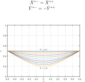
The superscript ∗ denotes the cyclic motion. Since the orbital energy is constant during one step, the relationship between the final velocity and the initial velocity for a cyclic motion is: ˙ X∗−= ˙X∗+ ˙ Y∗−= − ˙Y∗+ (8) -0.5 -0.4 -0.3 -0.2 -0.1 0 0.1 0.2 0.3 0.4 0.5 X 0 0.2 0.4 0.6 0.8 1 Y T = 0.1 T = 1.0

Fig. 2: Periodic motions in normalized variables for several values of T , orientation of the final velocity is defined by α. Considering the relationship between the final velocity and the initial velocity for cyclic motion described in equation(8), the initial velocity of CoM for a periodic motion of period T can be pointed out from equation(2):

˙ X∗+= ω1 + cosh(ωT ) 2 sinh(ωT ) ˙ Y∗+= ω1 − cosh(ωT ) 2 sinh(ωT ) (9)

In normalized variables, the cyclic motion for different values of time duration T is presented in Fig.2.

We characterize the orientation of the velocity at the end of the periodic single support phase by α = Y˙_˙∗−

X∗−. For cyclic

motion in normalized coordinates: α = −1−cosh(ωT )_{1+cosh(ωT )}, 0 < α < 1. During a step, the motion should start with an initial velocity that ˙X+_{> 0 and ˙Y}+_{< 0.}

For the 3D LIP model, the eigenvalues of the Poincaré map at the fixed points are {λλλ, 1}, where λλλ is the set of eigenvalues except of the one respect to kinetic energy. And if ∀|λi| ∈ λλλ < 1, the symmetric periodic orbits are

self-synchronized. This means that the period of oscillations in the x direction eventually matches that in the y direction, and the 3D LIP biped follows a periodic orbit. The other eigenvalue, which is 1, corresponds to neutral stability in kinetic energy. That is, if a small perturbation is applied to the 3D LIP, it will still become synchronized but will eventually follow a periodic orbit with a different level of kinetic energy. For stability, all the eigen values must be strictly less than one in norm.

D. The swing foot motion

A normalized variable Φ varying from zero to one, named phasing variable needs to be defined to describe the trajectory of the swing foot.

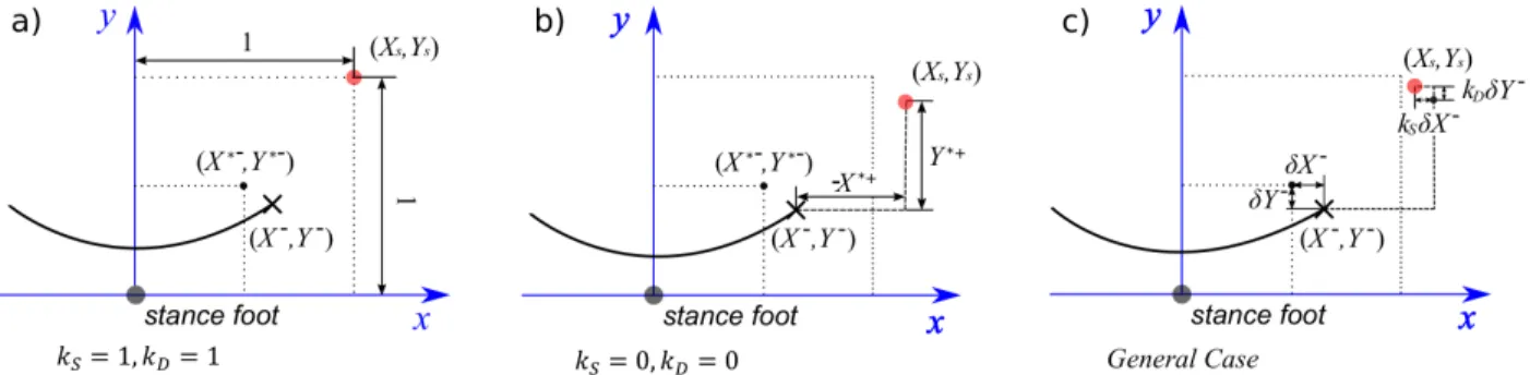
The position where to land the swing foot must be chosen cautiously. In this paper, in order to analyze all the possible cases in between, the pose of the swing foot at the end of a step is expressed in a generalized form:

X_s,k− = (1 − kS)(Xk−− 0.5) + 1

Y_s,k− = (1 − kD)(Yk−− 0.5) + 1

(10) where 0 ≤ kS ≤ 1 and 0 ≤ kD ≤ 1. How the parameters

kS and kD affect the placement of swing foot is illustrated

in Fig.3. With this choice, we can deduce the expression of the error in position of the CoM (δX = X − X∗) through the change of support:

δX_k+1+ = kSδXk−

δY_k+1+ = −kDδYk−

(11) The case kS = kD = 0 allows to nullify the error in

position through the change of support, while the case kS=

kD= 1 corresponds to a desired fixed step length and width

independently of the position of the CoM at the end of the step.

E. Switching condition

In this paper, we chose that the robot accepts to change of support when the CoM crosses the switching manifold S defined to be a line as function of C, as shown in Fig.4.

S = {(X, Y )|(X − 0.5) + C(Y − 0.5) = 0} (12) Many other sets of position can be considered but since stability studied in this paper is a local condition, a line is a convenient choice.

Fig. 3: Influence of kS and kD on the foot locations. a) Step length and width are fixed; b) The initial CoM position error

is nullified; c) The general case. The black and the red dots represent respectively the stance feet during the current and the next steps. The curved line represents the CoM trajectory, and the cross the CoM position at the end of the current step.

Fig. 4: The step is stopped when the CoM crosses the switching manifold (X − 0.5) + C(Y − 0.5) = 0, which is shown by the red line in the figure. The dashed line is the cyclic motion.

In presence of perturbation, the final CoM position error satisfies:

δX_k−+ CδY_k−= 0 (13) For a chosen evolution of the swing leg, the initial position of CoM can be deduced.

II. CALCULATION OFJACOBIANMATRIX FOR GENERAL CASES

To study the stability of the walking gait, the Poincaré return map is used. Since X_k− and Y_k− are coupled via the switching manifold (12), and the dynamic is autonomous (the time does not appear), the chosen independent state variables are (X_k−, L−_k, K_k−). The Jacobian is defined for a given periodic motion, and is characterized by the direction of the velocity of the CoM α.

Due to the existence of disturbance, the initial state of the robot after step k is written as:

X_k+ = X∗++ δX_k+ Y_k+ = Y∗++ δY_k+ ˙ X_k+ = X˙∗++ δ ˙X_k+ ˙ Y_k+ = Y˙∗++ δ ˙Y_k+ (14)

where X0 = −1₂, Y0 = 1₂. At the end of the step, the state

of the robot is denoted as:

X_k− = −X∗−_{+ δX}− k Y_k− = Y∗−+ δY_k− ˙ X_k− = X˙∗−_{+ δ ˙X}− k ˙ Y_k− = − ˙Y∗−+ δ ˙Y_k− (15)

Using the fact that X˙0 and ˙Y0 define a synchronized

motion and neglecting the second order terms, we obtain: Lk = δ ˙XkY˙0+ ˙X0δ ˙Yk−

ω2

2 (δXk− δYk) (16) We will now express the final error in velocity as function of the initial error for the step k. As the orbital energies, Ex and Ey and synchronizaiton measure L are conserved

quantities, we have: ( ˙X_k−)2− ω2_(X− k) 2_{= ( ˙X}+ k) 2_{− ω}2_(X+ k) 2 ₍₁₇₎ ( ˙Y_k−)2− ω2(Y_k−)2= ( ˙Y_k+)2− ω2(Y_k+)2 (18) ˙ X_k−Y˙_k−− ω2_X− kY − k = L − k (19)

Submit equation (14) and (15) into equation (17), (18) and (19) and neglect the second order terms, we can obtain:

(δ ˙X_k−)2+ 2δ ˙X_k−X˙0+ ˙X02− ω2 4 − ω 2_δX− k − ω 2_(δX− k) 2₌ (δ ˙X_k+)2+ 2δ ˙X_k+X˙0+ ˙X02− ω2 4 + ω 2_δX+ k − ω 2_(δX+ k) 2 (20) (δ ˙Y_k−)2− 2δ ˙Y_k−Y˙0+ ˙Y02− ω2 4 − ω 2_δY− k − ω 2_(δY− k ) 2₌ (δ ˙Y_k+)2+ 2δ ˙Y_k+Y˙0+ ˙Y02− ω2 4 − ω 2_δY+ k − ω 2_(δY+ k ) 2 (21) L−_k = ˙X0δ ˙Y_k−− δ ˙X_k−Y˙0− ω2 2 (δX − k + δY − k ) (22)

Using these equations and neglecting the second order terms, we obtain: δ ˙X_k−= ω 2 2 ˙X0 (δX_k−+ δX_k+) + δ ˙X_k+ (23) δ ˙Y_k−= ω 2 2 ˙Y0 (−δY_k−+ δY_k+) − δ ˙Y_k+ (24)

Submit equation (23) and (24) into equation (22) and rearrange it, we obtain:

(1 − 1 α)δY − k + (1 − α)δX − k = αδX_k+−δY + k α − 4Lk ω2 − δX + k + δY + k (25)

Because of the fact that:

δX_k−= −CδY_k− (26) δX_k+=kSC

kD

δY_k+ (27) Thus replace δY with δX in equation (25) and rearrange it, we obtain: (−1 + α)(1 + αC) α δY − k = (−1 + α)(αCkS+ kD) αkD δY_k+−4Li ω2 (28)

From the geometric relationship, we know that:

δX_k+1+ = kSδXk− (29)

δY_k+1+ = −kDδYk− (30)

Thus, from equation (28), we can obtain: − [1 −1 α− C(1 − α)]δX + k+1= (kSC kD α − 1 α− kDC kD + 1)δX_k+−4LikSC ω2 (31) and then: δX_k+1+ = −kD+ αCkS 1 + αC δX + k + 4αCkS ω2_{(−1 + α)(1 + αC)}Lk (32) From equation (28), we know that:

δX_k−= −C( −4αLk ω2_{(−1 + α)(1 + αC)} + kD+ αCkS kD+ αCkD δY_k+ (33) δY_k−= −4αLk ω2_{(−1 + α)(1 + αC)} + kD+ αCkS kD+ αCkD δY_k+ (34) Submit equation (33) and (34) into equation (23) and (24), we obtain: δ ˙X_k−= δ ˙X_k++ 2CαLk ˙ X0(−1 + α)(1 + αC) +ω 2_δX+ k 2 ˙X0 − Cω2_(k D+ αCkS)δYk+ 2(kD+ αCkD) ˙X0 (35) δ ˙Y_k−= −δ ˙Y_k++ 2αLk ˙ Y0(−1 + α)(1 + αC) + αω2C(kD− kS) 2(1 + αC)kDY˙0 δY_k+ (36)

For the step k + 1, the synchronization measure is: L−_k+1= ˙X0δ ˙Yk+1− − δ ˙X − k+1Y˙0− ω2 2 (δX − k+1+ δY − k+1) (37)

Submit equation (35) and (36) into (37) and rearrange it,

we obtain the relationship between Lk+1, Lk and δXK+:

Lk+1= (1 + α)(αC − 1) − 2α(kD− CkS) (1 − α)(αC + 1) Lk+ [(−2 + C)kD+ Cl](kD+ αCkS)ω2 2(1 + αC)CkS δX_k+ (38)

In conclusion, the Jacobian matrix is:

J =    −kD+αCkS (kS+αC) 4αCkS ω2_{(1+αC)(α−1)} 0 J21 2α(kD−Ck_{(1+αC)(α−1)}S)+(1−αC)(α+1) 0 ∗ ∗ 1    (39) with J21= (kD+αCkS)(−1+C+CkS−kD)ω2 2(1+αC)CkS .

III. STABILITY STUDY. A. Particular case :kD= kS = 0

In order to nullify the error in pose for the CoM at the beginning of step, kDand kS are supposed to be zero. Thus

the Jacobian becomes

J =    0 0 0 α(−1+C)ω2 2(1+αC) (−1+αC)(α+1) (1+αC)(1−α) 0 ∗ ∗ 1    (40) It has to be noted that with the proposed control strategy (the initial error in position of CoM is null), the decrease of synchronization measure, at the first order, is independent of the direction of the velocity error.

The eigen values are λ1 = 0, λ2 = 1 and λ3 = (−1+αC)(α+1)

(1+αC)(1−α) . The term

(1+α)

(1−α) is always greater than 1 for

0 < α < 1, its diverging effect increases when α increases. A condition on C to have synchronization can be easily deduced to meet the condition:

− 1 < (−1 + αC)(α + 1)

(1 + αC)(1 − α) < 1 (41) which gives:

1 < C < 1

α2 (42)

The condition λ3 < 1 ensures convergence toward a

syn-chronized motion, thus is a condition of self-synchronization. B. Particular case :kD= kS = 1

When kD = kS = 1, the step width and length are not

modified. The Jacobian becomes

J =    −1 4αC ω2_{(1+αC)(α−1)} 0 (−1+C)ω2 C 2α(1−C)+(1−αC)(α+1) (1+αC)(α−1) 0 ∗ ∗ 1    (43) The eigen values of the Jacobian are λ1= 1 and λ2, λ3=

(1+α)(1−αC)±2√α(−1+C)(−1+α2_C)

(1+αC)(α−1) .

When the eigen-value are complex, thus when α(−1 + C)(−1 + α2_{C)(α + 1) < 0 , it can be shown that the}

norms of the eigenvalues are strictly equal to 1, in the other cases at least one eigen value has a norm greater than 1. No synchronization can be achieved.

Proof: When α(−1 + C)(−1 + α2C)(α + 1) < 0, the square of the norm of the second eigenvalue equals to

(λ2)2 =

((1+α)(1−αC))2_{−4α(−1+C)(−1+α}2_C)

(1+αC)2_(α−1)2

= 1 (44)

C. Particular case :kD= 1, kS < 1

In this case, since the step width is not modified, the robot walks along the axis x without deviation.

The Jacobian becomes

J =    −1+αCkS 1+αC 4αCkS ω2(1+αC)(α−1) 0 J21 (−1+αC)(α+1)−2α(1−Ck_{(1+αC)(α−1)} s) 0 ∗ ∗ 1    (45) where J21=(−2+C+CkS)(1+αCkS)ω 2 2C(1+αC)kS . D. Particular case :kD≤ 1, kS = 0

In this case, the error in x direction at the beginning of a step is nullified, there is no connection between X_k+ and X_k+1+ . Thus instead of X, Y is considered in the Jacobian matrix and it needs to be calculated specifically.

J =    − kD(ω2+αω2) (−1+α)(1+αC)ω2 4αkD (−1+α)(1+αC)ω2 0 (−1+C−kD)ω2 2+2αC 1+α−α(1+α)C+2αkD (1+αC)(α−1) 0 ∗ ∗ 1    (46) For the case where kS = kD = 0, it is very simple to

analyze the synchronization because the Jacobian of Poincaré return map is a triangular matrix. However, the feet will not converge to their initial position. On the other hand, if we chose a constant position for landing the swing foot, the synchronization or stability is hard to achieve. For all these cases, the eigenvalues of the Jacobian matrix can be calculated symbolically.

REFERENCES

[1] S. Kajita, F. Kanehiro, K. Kaneko, K. Yokoi, and H. Hirukawa, “The 3d linear inverted pendulum mode: A simple modeling for a biped walking pattern generation,” in Intelligent Robots and Systems, 2001. Proceedings. 2001 IEEE/RSJ International Conference on, vol. 1. IEEE, 2001, pp. 239–246.

[2] S. Kajita, T. Yamaura, and A. Kobayashi, “Dynamic walking control of a biped robot along a potential energy conserving orbit,” IEEE Trans. Robot. Autom., vol. 8, no. 4, pp. 431–438, 1992.

[3] H. Razavi, A. M. Bloch, C. Chevallereau, and J. W. Grizzle, “Restrict-ed discrete invariance and self-synchronization for stable walking of bipedal robots,” in American Control Conference (ACC), 2015. IEEE, 2015, pp. 4818–4824.

[4] ——, “Symmetry in legged locomotion: a new method for designing stable periodic gaits,” Autonomous Robots, vol. 41, no. 5, pp. 1119– 1142, 2017.