HAL Id: halshs-01828633
https://halshs.archives-ouvertes.fr/halshs-01828633
Preprint submitted on 3 Jul 2018
HAL is a multi-disciplinary open access archive for the deposit and dissemination of sci-entific research documents, whether they are pub-lished or not. The documents may come from teaching and research institutions in France or abroad, or from public or private research centers.
L’archive ouverte pluridisciplinaire HAL, est destinée au dépôt et à la diffusion de documents scientifiques de niveau recherche, publiés ou non, émanant des établissements d’enseignement et de recherche français ou étrangers, des laboratoires publics ou privés.
Factors behind the Freight Rates in the Liner Shipping
Industry
Nikola Kutin, Zakaria Moussa, Thomas Vallée
To cite this version:
Nikola Kutin, Zakaria Moussa, Thomas Vallée. Factors behind the Freight Rates in the Liner Shipping Industry. 2018. �halshs-01828633�
EA 4272
Factors behind the Freight Rates in
the Liner Shipping Industry
Nikola Kutin*,**
Zakaria Moussa*
Thomas Vallée*
2018/08
(*) LEMNA - Université de Nantes
(**) National University of Management (Cambodge)
Laboratoire d’Economie et de Management Nantes-Atlantique Université de Nantes
Chemin de la Censive du Tertre – BP 52231 44322 Nantes cedex 3 – France http://www.lemna.univ-nantes.fr/ Tél. +33 (0)2 40 14 17 17 – Fax +33 (0)2 40 14 17 49
Docum
ent
de Tra
vai
l
W
or
ki
ng P
ape
r
1
Factors behind the Freight Rates in the Liner Shipping Industry
Nikola KUTINa, Zakaria MOUSSAb, Thomas VALLÉEc
a. LEMNA, IAE-Nantes, University of Nantes, Nantes, France and National University of Management, Phnom Penh, Cambodia, E-mail: [email protected] /
b. LEMNA, IAE-Nantes, University of Nantes, Nantes, France, E-mail:
c. LEMNA, IAE-Nantes, University of Nantes, Nantes, France, E-mail:
Acknowledgements
We would like to thank Mr. Tom Becker for reviewing this paper.
Abstract
This paper analyses the relationship between the China Containerized Freight Index (CCFI),
Containership Earnings, Fleet Development, bunker price and Global Economic Activity. The
Markov-switching Vector Autoregressive model has been applied by assuming the existence of
two regimes. The first one is characterized by low and volatile freight rates, while the second one
is more stable with high earnings and high freight rates. Three major cycles in the liner shipping
industry have been identified. Moreover, by applying the Impulse Reponses Function, we have
estimated the reaction of the freight rates following an increase of 1% of the other variables in
the model.
Date of final version: April 27, 2018
2
1. Introduction
Maritime transport is of major importance for the world’s economy as over 80% of the world’s trade is carried by sea (UNCTAD, 2017). It is the cheapest and most efficient way to transport goods in large quantity. Since the 1960s, containerization has greatly reduced the
expense of international trade and increased its speed, especially in consumer goods and commodities. It has also dramatically changed the ports’ infrastructures and shipbuilding industry. Even though in 2016, containerized cargo accounted for only 16.7%1 of the total
volume of transported goods, its value is more than 60%2. According to data of Clarkson
Research, since 1990, the containerized trade has increased by more than 600%.
However, the industry can be characterized by a high level of vulnerability and cyclic
pattern. Following the Subprime crisis, in 2009 container prices fell by 14% (UNCTAD, 2009)
which was caused by the dramatic decrease of 10.8% of the cargo transported in containers. It
was the first time since the invention of the containers that the World GDP grew faster than the
World Seaborne Container Trade. Since then, the industry has been in an unstable state. In the
last years, freight rates have been very low, ship values have plummeted and competition on the
various trade routes has intensified (Rex et al., 2016). In February 2017, the 7th biggest shipping
company Hanjin Shipping declared bankruptcy. It is a clear sign that even the big players in the
industry are threatened by the current situation.
1 Estimated by the authors based on the data collected from Clarkson Research Shipping Intelligence and UNCATD official websites.
3
Figure 1 Containership Fleet Growth and Idle Capacity: Source: Clarkson Research
Prior to the subprime crisis, the price of oil was steadily increasing (Figure 1). On some
major routes, shipping lines undertook different strategies with regard to the commercial speed
of the fleet and the scale of the vessels (Notteboom and Vernimmen, 2009). Notteboom and
Cariou (2009) estimated that by increasing the speed by two knots on average the fuel cost
increases by around 40%. The high fuel prices gave incentives to shipping companies to invest in
bigger ships and increase the time of travelling by reducing the speed and deploying more ships
on some maritime routes. After the world crisis and the slowdown of the world economy, the
excessive capacity seemed to have been a major concern for the industry. As shown in Figure 1,
global idle container ship capacity represented 11.4% in January, 2010 and despite the
decreasing trend of the fleet growth, it has remained relatively high (5.64% in March, 2017).
Freight Rates in the containerized industry have a direct impact on the shipping lines
decisions and world trade. They can be defined as the price for transporting a standard 20-foot
4
factors behind the freight rates is not an easy task. The complexity arises from the fact that a
large number of parties, each one with different objectives, is involved in container shipping
(that is consignor, a consignee, an ocean carrier, freight forwarders, inland carriers, banks, legal
experts, insurance brokers, customs, port/terminal operators, and inland depot operators). Lee
and Song (2017) classified them into service users and service providers. In addition, Container rates are quoted as the price per box, “Freight all Kinds”. This makes it even more complex to generalize how rates are structured spatially, because the tarification is not related to the product
being transported as in some other trades (Slack and Gouvernal, 2011).
Container freight rates can be broken down into three main components: Basic Ocean
Freight (BAS), Mandatory surcharges and Value Added Services (VAS). BAS is mainly
determined by the origin and destination of the cargo. Mandatory surcharges include a variety of
charges that are added to BAS. For instance Bunker Adjustment Factor take into account the
variation of the cost spent on fuel while Terminal Handling Charges are based on the cost of
handling a container. Finally, VAS is related to the requirements of any particular client.
Examples of such services are container cleaning and cold treatment. According to Maersk Line,
BAS accounts for 50%, Mandatory surcharges for 25% and VAS for 25%3. Slack and Gouvernal
(2011) found out that surcharges account for more than 50% in the total freight charged to
customers.
The objective of this paper is to analyze the relationship between key variables in the
liner shipping industry by taking into account its cyclical and nonlinear patterns. Firstly, we
depict some key findings and gaps in the literature regarding the ocean freight rates. Secondly,
the methodology of Markov-Switching Vector Autoregressive (MS-VAR) models and the
3 Freight shipping rates and container costs, Official Website of Maersk Line
5
Impulse Response function are presented along with detailed description of each one of the
selected variables. Thirdly, a detailed explanation of the different regimes as well as their
switching probability are explained. This section of the paper also describes the six economic
cycles that have been identified and the impulse responses of China Containerized Freight Index
(CCFI) following a shock of another variable in the model. Finally, a summary of the main
findings and possibility of future research are provided.
2. Literature Review
Since the Subprime Crisis, freight rates in the liner shipping industry have been very
volatile and many empirical studies have been conducted to understand its behavior. De Oliveira
(2014) applied different methods of regressions, such as the random effects (RE) and fixed
effects (FE), and the Hausman–Taylor (HT) estimator to analyze the freight rates. His study
included 1,128 quotations for transporting a standard 20-foot container between six European
countries and 47 partners. The independent variables in his model were the port-to-port distance,
number of transshipments, economies of scale and Liner Shipping Connectivity Index. The
results show that inward freight rates are on average, 23% higher than for outward ones, with the
competition having a strong effect on the freight rates and surcharges appearing to be one of the
main revenue-makers.
Slack and Gouvernal (2011) analyzed the factors behind the freight rates in the case of 35
port destinations from Northern Europe. Their study shows that that distance is not a factor in
explaining freight rates and the regional and temporal differences do not have any significant
impact on the price of shipments. They also found that there is no correlation between the
distance and BAF and no significant relationship between freight rates, imports and size of the
6
Behrens and Picard (2011) suggested that the impact of globalization as well as regional
disparities on freight rates are overstated. The main reason for asymmetric freight rates is the
presence of empty containers. Lun et al. (2013) used Path analysis in Structural Equation
Modeling (SEM) to analyze the causality between the following variables: container trade, total
fleet, freight rate, new building vessel price, second-hand vessel price, and demolition vessel
price. The data is weekly for a period of twelve years, collected from Clarkson Research. Results
suggest that there is significant relationship between total Fleet size and seaborne trade and no
link between freight rate and seaborne trade. Tran and Haasis (2015) applied multiple regression
to analyze the costs and revenues of the top 25 Container Operators. They found that market
freight rate has an effect on revenue and the capacity has an impact on the total cost of the
operators. Ordinary Least Square method was used by Duru and Yoshida (2011) to investigate
the factors behind the Long term composite Freight Index (LFI), created by them and the
seaborne trade. Their study shows that life expectancy is significant for both the models while
the effect of fleet size is very weak.
Considering the nonlinear relations between the different factors influencing freight rates
and their interdependence, some authors have applied different autoregressive models. Veenstra
and Franses (1997) used the Multivariate Cointegration approach to analyze the relationship of
six bulk freight rates related to different commodities and routes. A cointegration between five of
the variables in the model was found and a VEC model was formulated. The stochastic trend of
all variables show that an important part of the pattern of the freight rates cannot be predicted.
Veenstra (1999) used the VAR model to examine the relation between spot and period freight
rates for the ocean dry bulk shipping market. The research show the evidence of a term structure
7
(2016) applied the ARDL approach to build export and import models regarding the trade
between China and US. Results reveal that gross domestic product is the key determinant of
bilateral freight flows, while the real income is closely related to the bilateral freight flows. They
also found that transport costs can be an important factor affecting the inflows of Chinese
commodities to the US.
However the cyclic nature of the freight rates should also be considered. An appropriate
approach is Markov Switching Vector Autoregressive model (MS-VAR) which allows us to
analyze the relationship between the variables according to different states of the market. There
are very few studies that have applied such a methodology in the context of ocean freight rates.
Bildirici et al. (2015) analyzed the relation between GDP growth in US and the Baltic Dry Index
(BDI) by assuming the existence of three regimes. The first one is associated with the crisis, the
second one is the moderate growth regime and the third one is the high growth regime. They
found that under the high growth regime, BDI improvement effects economic growth positively.
As seen from the literature review, most of the authors have focused on the ocean bulk
freight rates. We have not found any study applying VAR methods to investigate the freight rates
in the container trade. VAR modeling is widely applied in macroeconomics because it does not
require as much knowledge about the forces influencing a variable as structural models with
simultaneous equations. Its main advantage is that all variables are treated as endogenous and
each one is explained by its lagged values, the lagged values of the other variables in the model
and error terms. Thus, we can analyze the linear interdependence among multiple time series by
avoiding the problem of endogeneity (an explanatory variable is correlated with the error term).
A standard approach of VAR modelling is the estimation of the impulse responses function of
8
and Watson, 2001). Considering the current volatile freight rates and the oversupply in the
industry, it is also important to investigate the potential structural changes in the containerized
trade market.
Our paper aims to fill in this gap in the literature and to provide empirical application of
MS-VAR and impulse responses function in the context of containerized trade market. The
objective of the research is to identify the different business cycles that have occurred in the liner
shipping industry in the last 13 years and to analyze their nature as well as to evaluate the effects
on the container freight rates following a surprising increase in the oil price, earnings, Fleet
Development or Global Economic Activity.
MS-VAR provides accurate estimates regarding the duration of each regime as well as
the switching probabilities. Moreover, it allows one to distinguish different business cycles
occurring during the observed period. For each regime we have computed the impulse responses
of CCFI following a positive shock of another variable in the model.
3. Methodology 3.1. MS-VAR model
Following the pioneer work of Sims (1980), VAR modeling has become a useful tool in
macroeconomics. Contrary to the structural models with simultaneous equations, VAR avoids
the problems of over-identification (differentiating between correlation and causation by
imposing restrictions). In VAR models, variables are endogenous. VAR provides a coherent and
credible approach to data description, forecasting, structural inference, and policy analysis. In
9
containerized market operates, we combine the VAR approach with the Markov Chain process in
the so-called Markov-switching Vector Autoregressive (MS-VAR) modelling.
Following Hamilton (1989), the general MS-VAR is depicted by equations (1) where it is
assumed that a change in regime corresponds to an immediate one-time jump in the process
mean. The description of MS-VAR in the current paper follows (Ehrmann et al., 2003). In our
model, we consider that the mean would smoothly approach a new level after the transition from
one regime to another. We do it in an extension of Hamilton’s approach to a regime-switching
VAR system (Krolzig, 2013).
where refers to China Containerized Freight Composite Index (CCFI),
West Texas Intermediate oil price, Clarksons Average Containership Earnings, Total
Containership Fleet Development and Index of Global Economic Activity. These exogenous
variables are explained by an intercept , autoregressive terms of order ρ and a residual .
The number of regimes in the model is two, , and all parameters are allowed to switch
between the regimes. Therefore, each of the two regimes is defined by an intercept ,
autoregressive term and matrix .
After the change in regime there is thus an immediate one-time jump in the variance of
errors. This model is based on the assumption of varying processes according to the economic
10
model is assumed to follow the discrete time and discrete state stochastic process of a
hidden Markov chain and governed by transition probabilities , and
. The conditional probabilities are collected into a transition matrix P
as follows:
(2)
For a given parametric specification of the model, probabilities are assigned to the
unobserved regimes conditional on the available information set which constitutes an optimal
inference on the latent state of the market (Girardin and Moussa, 2011). We thus obtain the
probability of staying in a given regime when starting from that regime, as well as the probability
of shifting to another regime. The classification of regimes and the dating algorithm used imply
that every observation in the sample is assigned to one of the two regimes. We assign an
observation to a specific regime when the smoothed probability of being in that regime is higher
than 50%. The smoothed probability of being in a given regime is computed by using all the
observations in the sample.
3.2. Impulse Response Function
In a MS-VAR model, with regime-dependence in the mean, variance and autoregressive
parameters, a large number of parameters can switch between regimes. Ehrmann et al. (2003)
suggest the use of regime-dependent impulse response functions which allow the investigation of
how fundamental disturbances affect the variables in the model. For each regime, there is a set of
impulse response functions. Each response function depends on the prevailing regime at the time
of the shock. They facilitate the interpretation of switching parameters by providing a convenient
11
covariances of each regime (Girardin and Moussa, 2011). We follow the method of identification
and estimation of impulse response proposed by Ehrmann et al. (2003).
There are regime-dependent impulse response functions which correspond to the
reaction of variable to disturbances in regime .
(3)
Equation 3 shows the mathematical representation of the impulse response function for
regime . It reveals the expected changes in endogenous variables at time to one standard
deviation shock to the -th fundamental disturbance at time in regime . A series of
dimensional response vectors predict the response of the endogenous variables.
In order to make the precision of the impulse responses function more accurate, the
bootstrapping technique was applied. This technique is used to create artificial observations for
the variables and use them for the same estimation procedures as the original dataset. The
artificial histories are created by replacing the parameters in the model with their estimated
variance-covariance matrix, and then calculating the endogenous variables (Ehrmann et al.,
2003). However, in MS-VAR, applying the bootstrapping technique is complicated due to the
existence of a hidden Markov-chain process which determines the regimes. Therefore, we first
create a history for the regimes, and then we use it to continue for the endogenous variables.
Ehrmann et al. (2003) proposed the following five steps to apply bootstrapping technique in the
context of MS-VAR. Firstly, a history for the hidden regime is created by replacing the
exogenous transition matrix with its estimated value . At each time , a random number is
drawn from a uniform [0,1] distribution and compared with the conditional transition
12
endogenous variables is generated. All parameters in Equation 1 are replaced by their estimated
values and new residuals are computed. Thirdly, we use the data of the artificial history to
compute bootstrapped parameters for , the transition matrix , and
the smooth probabilities Fourthly, a set of
restrictions are imposed which provide bootstrapped estimates of the matrices .
Finally, the bootstrapped estimates of the response vectors are computed.
3.3. Data
The following data have been selected: China Containerized Freight Composite Index
(CCFI), Clarksons Average Containership Earnings ($/Day), Total Containership Fleet
Development (thousand TEUs), West Texas Intermediate oil price ($/bbl) and the updated
version of the index of global real economic activity. In total, there are 168 observations. The
first three variables were collected from Clarksons Shipping Intelligence Network. Statistics
regarding the price of crude oil were provided by the Energy and Information Administration of
US (https://www.eia.gov/). The Global Real Economic Activity index was computed by (Kilian,
2009).
- China Containerized Freight Composite Index - CCFI (Index)
China (Export) Containerized Freight Index (CCFI) is sponsored by the Ministry of
Communications of China and formulated by the Shanghai Shipping Exchange. The index serves
as a barometer of the liner shipping industry and it is computed based on data collected from 22
major international and domestic shipping companies for 11 major ports of departure in China.
13
representatives of major domestic and foreign shipping companies. This is the key variable in the
research and it is denoted as CCFI in our analyses.
- Clarksons Average Containership Earnings ($/Day)
Clarksons Average Containership Earnings is based on information provided by
Clarksons brokers on a daily and weekly basis. This information is used to calculate the earnings
in the liner shipping industry by taking into account the number of the fully cellular
containerships. Clarkson Research compute earnings based on a single freight rate. This indicator
is a proxy for the profitability in the container shipping industry. In our research, this variable is
denoted as “Earnings”. In broad terms, earnings for each route are calculated by taking the total
revenue, deducting current bunker costs based on prices at representative regional bunker ports,
estimated port costs (after currency adjustments) and total commission and then dividing the
result by the number of voyage days (Clarkson Research, 2015).
- Total Containership Fleet Development (Thousand TEUs)
The size of all containerships is estimated in TEUs. This variable refers to the supply of
the Liner Shipping. In the current paper we refer to this variable as “Fleet”.
- West Texas Intermediate oil price ($/bbl)
West Texas Intermediate, also known as Texas light sweet, is a grade of crude oil used as
a benchmark in oil pricing. The bunker cost accounts for 70% of the operational cost of carriers
and thus WTI could be used as a proxy for the operational costs of the carriers.
14
The index of global real economic activity is computed from data collected from the
monthly report on "Ship and Economics" published by Drewry Shipping Consultants Ltd. It is
based on a global index of dry cargo single voyage freight rates of various bulk dry cargos such
as grain, oilseeds, coal, iron ore, fertilizer, and scrap metal. The index can be traced back to 1968
and it is a direct measure of global economic activity which does not require exchange-rate
weighting. It automatically aggregates real economic activity in all countries and incorporates
shifting country weights, changes in the composition of real output, and changes in the
propensity to import industrial commodities for a given unit of real output (Kilian, 2009).
4. Empirical Results 4.1. Descriptive statistics and specifications of MS-VAR
We use monthly time series from March 2003 to February 2017. Table 1 provides a
summary of the descriptive statistics for all variables. The average values of all indicators are
positive. Standard Deviation is very high for the Crude oil, Earnings, and Global activity.
According to the results of Skewness and Kurtosis, most of the variables are symmetrically
distributed except CCFI and Global Activity. In addition, the Jarque–Bera test confirms these
results and accepts the normality hypothesis. In order to check whether each variable follows a
unit-root process, we applied the Dickey–Fuller test. The unit root test of Augmented Dickey
Fuller test clearly rejects the null hypothesis of the stationarity of all variables except Global
Activity. It means that all variables except Global Activity have a unit root and are generated by
15
Table 1 Descriptive statistics
Correlation coefficients for the whole sample are presented in Table 1. It shows that all
variables in the model have a positive correlation with CCFI except the Fleet. However the
correlation coefficients are less than 50%. The strong and negative correlation between Earning
and Fleet (-0.80) suggests a possible negative effect of the growing capacity in the shipping
industry on the Earnings. There is also a negative correlation of 75% between Fleet and Global
Activity.
CCFI Earnings Fleet Crude Oil Global Activity
CCFI 1
Earnings 0.4369 1
Fleet -0.4613 -0.7975 1
Crude Oil 0.3906 -0.2051 0.2811 1
Global Activity 0.4553 0.6475 -0.7538 0.0962 1 Table 2 Correlation Matrix
In the MS-VAR model and impulse response functions, all variables were transformed
into log and we use their growth rates for our analysis. Following the results of the Augmented
Dickey–Fuller test, we also transform all variables into first difference, except Global Activity.
In the current paper we estimate an unrestricted MS-VAR model with intercept and without
trend. We choose 2 lags based on the AIC, HQ and SC criteria. We also assume the existence of
16
4.2. Business Cycles in the Liner shipping industry
As we have already emphasized, the MS-VAR model allows us to identify the different
business cycles that have occurred from May 2003 to February 2017 (we have included two lags
in the model). Figure 2 shows the transitional switching probabilities of regime 1 (the blue line)
as well as the value of the CCFI (the red line).
Figure 2 Smoothed probability of Regime 1 (volatile and decreasing freight Rates) and CCFI index. Source: Author’s drawing
In the MS-VAR model, all variables were transformed into log and we use their monthly growth rates. The blue line shows the switching probability of the more volatile Regime 1. The red line depicts CCFI.
Both regimes are very persistent as shown in the matrix below. The regime switching
probabilities for Regime 1 and Regime 2 are 18% and 17%, respectively. A major event that
marks the switch of the regime 2 to regime 1 is the Subprime Crisis. The switch occurs in
September 2008 and has a major impact on the variables in the model.
17
Throughout the observed period, Regime 1 and Regime 2 last 71 and 95 months,
respectively. Table 3 and Table 4 show the descriptive statistics of the variables under each of
the identified regimes. Regime 1 is characterized by lower average container freight rates and
considerably higher volatility (Standard Deviation). Moreover, under the second regime the
average Global Activity is negative (-15.2), while in regime one, its mean value is 29.32.
Earnings are also considerably higher under the second regime (15,908). On the other hand, the
mean and the standard deviation of the Fleet are higher in the first regime. It suggests, that
Regime 1 is characterized by a low level of economic activity, a high level of volatility of freight
rates, a low level of earnings and a high growth rate of the containership capacity. The second
regime is slightly more persistent than the first one and can be defined as a regime of a high level
of economic activity, high and stable container freight rates, a high level of earnings and a low
level of fleet capacity.
CCFI Earnings Fleet Crude Oil Global Activity
Min 641.50 4,619.34 11,926.45 30.32 -133.13 Max 1,263.72 1,5740.16 20,043.44 106.29 44.45 Average 943.04 7,310.74 16,677.73 69.88 -15.42 Std. Dev. 161.10 2,344.44 2,679.00 23.65 32.54 Med 956.77 6,461.60 17,084.64 69.64 -15.28 Kurtosis -1.12 1.85 -1.18 -1.62 1.66 Skewness 0.15 -1.47 0.32 -0.01 0.84
Table 3 Descriptive Statistics of Regime 1
CCFI Earnings Fleet Crude Oil Global Activity
Min 946.37 4,395.78 6,257.82 28.11 -29.43 Max 1,315.87 28,650.86 17,872.49 133.88 66.78 Average 1,097.40 15,908.95 10,642.82 71.30 29.32 Std. Dev. 74.32 6,906.49 3,524.77 25.72 25.35 Med 1,097.94 16,205.72 6,501.78 30.34 42.01 Kurtosis 0.50 -0.86 -0.92 -0.55 -0.22 Skewness 0.48 -0.16 0.57 0.24 -0.80
18
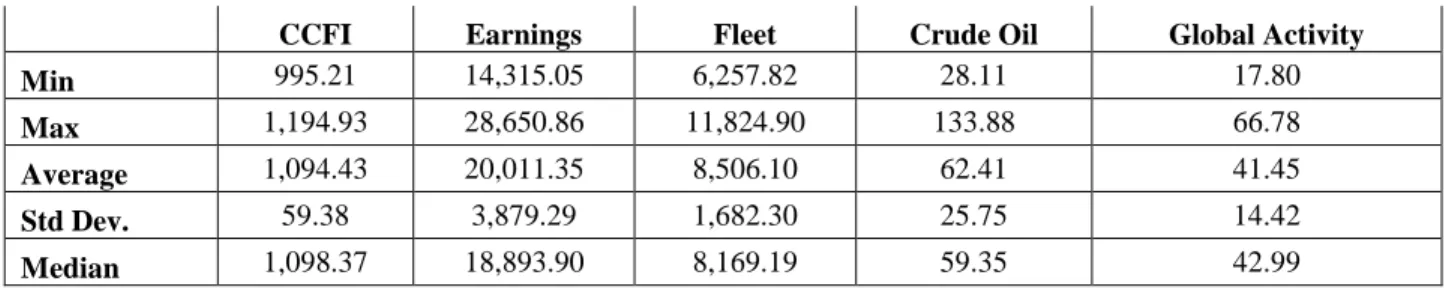
By looking at Figure 2 we can distinguish three economic cycles. The first one is from
May 2003 to August 2008 which falls under Regime 2. This period can be characterized by
steady growth, very low volatility of CCFI, a high level of earnings, a low price of crude oil and
a very high level of Global Activity (Table 5). This is the longest period which falls uniquely
under the second regime (64 months).
CCFI Earnings Fleet Crude Oil Global Activity
Min 995.21 14,315.05 6,257.82 28.11 17.80
Max 1,194.93 28,650.86 11,824.90 133.88 66.78
Average 1,094.43 20,011.35 8,506.10 62.41 41.45
Std Dev. 59.38 3,879.29 1,682.30 25.75 14.42
Median 1,098.37 18,893.90 8,169.19 59.35 42.99
Table 5 : Business Cycle 1: Steady Growth Descriptive statistics (May 2003 - August 2008)
The effect of the Subprime Crisis on Containerized trade started in September 2008,
when we have a switch from Regime 2 to Regime 1. This marks the beginning of the second
business cycle, which is characterized by a high level of uncertainty. This cycle continues until
August 2014 (72 months in total). Throughout this period we have frequent switches between the
two regimes. Even though the average CCFI has decreased by only 3% compared to the previous
cycle, its volatility has increased by 102%. Earnings and Global Activity also had a dramatic
decrease of 62% and 95%, respectively (Table 6). This period could be characterized as a
post-crisis period where government took considerable measures to support the industry and to
maintain economic growth. This business cycle lasts 72 months.
CCFI Earnings Fleet Crude Oil Global Activity
Min 777.04 4,395.78 11,926.45 39.09 -41.27
Max 1,315.87 15,740.16 17,872.49 109.53 44.45
Average 1,057.41 7,504.49 14,884.93 86.40 2.19
Std. Dev. 119.77 2,725.36 1,776.50 16.82 24.20
Median 1,066.60 6,537.33 15,066.53 89.33 2.69
19
From September 2014 to February 2017, we observe a business cycle which falls entirely
under Regime 1 and we have named it “The New Normal” which lasts 30 months. During this
period, the average Global Activity decreased by 39.52 points (Table 7). The average CCFI is
21% lower than the second business cycle and its volatility is 20% higher. Earnings became less
volatile and decreased by 7% compare to the previous cycle. The Fleet has increased by 30% and
its volatility is 58% lower. In April 2016, CCFI registered its lowest monthly value ever
recorded, 641.50 points, and in August 2016 the Hanjin Shipping, the seventh biggest shipping
company, declared bankruptcy.
CCFI Earnings Fleet Crude Oil Global Activity
Min 641.50 5,357.11 17,926.47 30.32 -133.13
Max 1,107.11 10,935.99 20,043.44 93.21 2.18
Average 834.42 6,978.76 19,302.69 50.69 -37.33
Std Dev. 143.40 1,729.89 743.40 13.65 30.08
Median 799.92 6,156.18 19,657.97 47.52 -33.49
Table 7: Business Cycle 3: The new Normal Descriptive statistics (September 2008 - August 2014)
The proposed MS-VAR model tracks well different cycles that have occurred in the liner
shipping industry. Both regimes are very persistent, which allows us to assume that the last business cycle, “The New Normal” might continue for at least a few more years. The growing number of conferences between carriers is a clear sign that shipping companies are trying to
minimize their costs in order to deal with the low world demand and high level of containership
capacity. We also observe a monopolization of the shipping market. According to Alphaliner, in
2008 Maersk had a share of around 6% of the world fleet, while in April 2017, it was more than
16%.
20
We use impulse response functions to show how the endogenous variables react to
shocks of one standard deviation of the residuals of each equation (Crude Oil, Earnings, Fleet or
Global Activity). The Impulse response functions are conditional on a given regime prevailing at
the time of the disturbance and throughout the duration of the response (Ehrmann et al., 2003).
In order to increase the precision of our estimation, we have applied the standard bootstrapping
techniques. This method consists of increasing the number of observations by creating artificial
histories for the variables. We have made 1000 bootstrap replications. Similarly to Uhlig (2005)
and considering the findings of Inoue and Kilian (2016), we use a confidence interval of 68%.
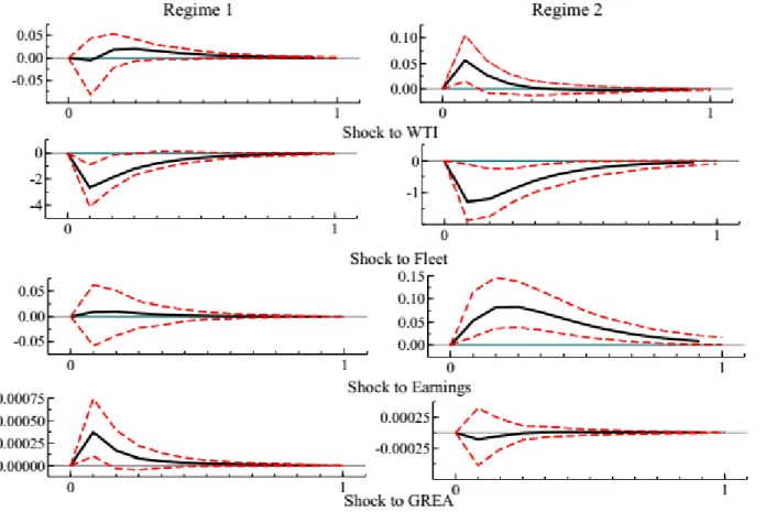
Figure 3: Response of CCFI reacting to shock to the other variables in the MS-VAR model according to the two regimes.
Note: The variables were transformed in log and we use their growth rate for the analysis. Impulse response functions of CCFI are conditioned to the prevailing regime. The figure depicts responses of CCFI to a positive shock of 1% to the other variables in the model. The impulse reaction period is chosen to be 12 months. Solid black lines
21
depict impulse responses of CCFI, while dashed lines depict 68% confidence intervals. The upper dashed and lower dashed lines represent 84% quantile and the 16% quantile of the posterior distribution, respectively. Impulse responses are computed on the basis of 1000 bootstrap replications. GREA refers to Global Real Economic Activity Index while WTI refers to the price of Crude Oil.
The response of CCFI to a one standard deviation shock to the other variables in the
model are shown in Figure 3. Responses are regime dependent: the left-hand diagrams
correspond to Regime 1 (high volatility and decreasing freight rates) whereas the right-hand
figures refer to Regime 2 (low volatility and high container freight rates).
A positive shock of 1% of the crude oil has a significant effect on CCFI only in the
second regime. This could be explained by the fact that most of the observations which fall under
the second regime (stable growth) are before September 2008. During that time, the oil price had
an increasing trend (see Figure 1) and thus the freight rates were strongly associated with the
bunker price. On the other hand, throughout Regime 1 which is post crisis regime, the price of
crude oil is quite low and has a decreasing trend.
The size of the world Fleet has substantial impact in both regimes. It is more pronounced
in Regime 1, where a 1% increase of the size of the fleet leads to an immediate 3% decrease of
the container freight rates. Then it takes around 7 months for CCFI to go to its equilibrium level.
In the second regime, the shock of the Fleet is also significant and CCFI decreases by
approximately 1.4%. These results suggest that the supply in the shipping industry plays a major
role in the container freight rate price formation. During a period of growth and low volatility,
companies are able to better plan their strategies in terms of fleet development, while during a
period of crisis, we have a substantial decrease in the demand for container transport which
drives the freight rates down. Shipping companies are trying to optimize their fleet by renewing
22
the monthly average of scrapped vessels were 3,257 TEUs, while from September 2009 to March
2017, the monthly average was 16,138 TEUs, which is the equivalent of one Triple E
containership. In January 2014, the equivalent of demolished ships was 84,740 TEUs, the highest
level ever recorded. We should emphasize that many environmental and safety regulations also
play a role in the increase of scrapping activities.
Earnings in the shipping industry are significant only under the regime of growth and low
volatility. A change in 1% in the level of earnings would lead to a 0.08% increase of CCFI. Even
though the impact on the container freight rates is not very great, it lasts for 12 months.
The last variable in the model, Index of Global Economic Activity (GREA), is significant
only in the First Regime of the impulse response function of CCFI. However, the effect of this
variable is not substantial and its duration is only 2 months. It is interesting to highlight the fact
that under the second regime, the function has a decreasing trend.
In appendices 1, 2, and 4 are presented the impulse response functions of Earnings, Fleet,
Global Activity and Crude Oil respectively. It is interesting to observe that CCFI has a very
substantial negative effect on Earnings in the case of both regimes. To a lesser extent, CCFI has
a positive impact on Global Activity and the price of crude oil.
5. Conclusion
This paper contributes to the existing literature by exploring the relationship between the
China Containerized Freight Index (CCFI), Clarksons Average Containership Earnings, Fleet
Development, the price of Crude Oil and Global Real Economic Activity by applying MS-VAR
23
and intercept by assuming the existence of two regimes. The first one can be characterized as a
regime of crisis, low freight rates and high volatility occurring after the Subprime crisis, while
the second one is a state of steady growth and low volatility in the shipping industry. The
identified regimes are very persistent and track well the trends and business cycles in the
shipping industry between May 2003 and February 2017. We have identified 3 major business
cycles. The first one is characterized by a period of long and steady growth which lasts until
August 2008. The following cycle is a transitional one which lasts 6 years. The third cycle is
characterized by very low freight rates, low earnings and substantial size of the world fleet.
The impulse responses methodology allows us to pin down the consistent and efficient
estimates of the reaction of CCFI to different factors according to the two states of the industry
(Regime 1 and Regime 2). The variable which has a profound negative impact on the container
freight rates is the growth of the world fleet. Its effect is more pronounced under the regime of
crisis. Earnings in the shipping market and the crude oil price are only significant in the second
regime and both have a positive impact on CCFI. The Global Economic activity has a minor
effect on CCFI in the regime of crisis.
Potential future research could include the use of another indicator as a proxy for freight
rates instead of CCFI. In this way we could double check our findings. Moreover, a variable
which depicts the market concentration in the liner shipping industry (for example, the share of
the top 10 companies in terms of transported TEUs) could also be included in the model. Other
variables which reflect the Economic activity worldwide such as the industrial production of
OECD member states could be also be considered.
The last identified economic cycle (“The New Normal”) is characterized by low
24
Shipping companies are dealing with this unstable prospect of the market by limiting their
operational costs (that is slow steaming strategies and economies of scale) and sharing capacity
(creation of alliances). As UNCTAD pointed out, the market has become more monopolized and
small players are vulnerable. In addition, even the big companies, such as Hanjin Shipping, could
face bankruptcy. When we take into account the regionalization of the trade (for example,
ASEAN Economic Community, Trade agreement between the EU and Canada, etc.) and the
slowdown of the Chinese economy, it is obvious that the current unstable situation of “New
25
References
Behrens, K. and Picard, P. M. (2011): 'Transportation, freight rates, and economic geography.
Journal of International Economics', 85, 280-291.
Bildirici, M. E., Kayıkçı, F. and Onat, I. Ş. (2015): 'Baltic Dry Index as a major economic policy indicator: the relationship with economic growth. Procedia-Social and Behavioral
Sciences', 210, 416-424.
Chi, J. (2016): 'Exchange rate and transport cost sensitivities of bilateral freight flows between
the US and China. Transportation Research Part A: Policy and Practice', 89, 1-13.
De Oliveira, G. F. (2014): 'Determinants of European freight rates: The role of market power and
trade imbalance. Transportation Research Part E: Logistics and Transportation Review',
62, 23-33.
Duru, O. and Yoshida, S. (2011): 'Long term freight market index and inferences. The Asian
Journal of Shipping and Logistics', 27, 405-421.
Ehrmann, M., Ellison, M. and Valla, N. (2003): 'Regime-dependent impulse response functions
in a Markov-switching vector autoregression model. Economics Letters', 78, 295-299.
Girardin, E. and Moussa, Z. (2011): 'Quantitative easing works: Lessons from the unique
experience in Japan 2001–2006. Journal of International Financial Markets, Institutions
and Money', 21, 461-495.
Hamilton, J. D. (1989): 'A new approach to the economic analysis of nonstationary time series
and the business cycle. Econometrica: Journal of the Econometric Society', 357-384.
Inoue, A. and Kilian, L. (2016): 'Joint confidence sets for structural impulse responses. Journal
26
Kilian, L. (2009): 'Not all oil price shocks are alike: Disentangling demand and supply shocks in
the crude oil market. American Economic Review', 99, 1053-69.
Krolzig, H.-M. 2013. Markov-switching vector autoregressions: Modelling, statistical inference,
and application to business cycle analysis, Springer Science & Business Media.
Kutin, N. and Vallée, T. (2015): Final report: Maritime and Inland Waterways Socioeconomic
Activities Observatory of Cambodia, Phnom Penh, Cambodia.
Lee, C.-Y. and Song, D.-P. (2017): 'Ocean container transport in global supply chains: Overview
and research opportunities. Transportation Research Part B: Methodological', 95,
442-474.
Lun, Y. V., Lai, K.-H., Wong, C. W. and Cheng, T. (2013): 'Demand chain management in the
container shipping service industry. International journal of production economics', 141,
485-492.
Notteboom, T. and Cariou, P. Fuel surcharge practices of container shipping lines: Is it about
cost recovery or revenue making. Proceedings of the 2009 international association of
maritime economists (IAME) conference, 2009. IAME Copenhagen, Denmark, 24-26.
Notteboom, T. E. and Vernimmen, B. (2009): 'The effect of high fuel costs on liner service
configuration in container shipping. Journal of Transport Geography', 17, 325-337.
Research, C. 2015. Sources and Methods for the Shipping Intelligence Weekly. Clarksons
Quality System Clarkson Research Services Limited.
Rex, C., Andersen, M. and Kristensen, N. (2016): Shipping market review, Danish ship finance.
Sims, C. A. (1980): 'Macroeconomics and reality. Econometrica: Journal of the Econometric
27
Slack, B. and Gouvernal, E. (2011): 'Container freight rates and the role of surcharges. Journal of
transport geography', 19, 1482-1489.
Stock, J. H. and Watson, M. W. (2001): 'Vector autoregressions. Journal of Economic
perspectives', 15, 101-115.
Tran, N. K. and Haasis, H.-D. (2015): 'An empirical study of fleet expansion and growth of ship
size in container liner shipping. International Journal of Production Economics', 159,
241-253.
Uhlig, H. (2005): 'What are the effects of monetary policy on output? Results from an agnostic
identification procedure. Journal of Monetary Economics', 52, 381-419.
Unctad. 2009. Review of Maritime Transport 2009.
Unctad 2017. Review of Maritime Transport 2017. Review of Maritime Transport. United
Nations Conference on Trade and Development.
Veenstra, A. W. (1999): 'The term structure of ocean freight rates. Maritime Policy &
Management', 26, 279-293.
Veenstra, A. W. and Franses, P. H. (1997): 'A co-integration approach to forecasting freight rates
in the dry bulk shipping sector. Transportation Research Part A: policy and practice', 31,
28
Appendices
Appendix 1: Response of Earnings reacting to shock to the other variables in the MS-VAR model according to the two regimes
Note: The variables were transformed in log and we use their growth rate for the analysis. Impulse response functions of Earnings are conditioned to the prevailing regime. The figure depicts responses of the Earnings to a positive shock of 1% to the other variables in the model. The impulse reaction period is chosen to be 12 months. Solid black lines depict impulse responses of Earnings, while dashed lines depict 68% confidence intervals. The upper dashed and lower dashed lines represent 84% quantile and the 16% quantile of the posterior distribution, respectively. Impulse responses are computed on the basis of 1000 bootstrap replications. GREA refers to Global Real Economic Activity Index while WTI refers to the price of Crude Oil.
29
Appendix 2 Response of Fleet reacting to shock to the other variables in the MS-VAR model according to the two regimes
Note: The variables were transformed in log and we use their growth rate for the analysis. Impulse response functions of Fleet are conditioned to the prevailing regime. The figure depicts responses of the Fleet to a positive shock of 1% to the other variables in the model. The impulse reaction period is chosen to be 12 months. Solid black lines depict impulse responses of Fleet, while dashed lines depict 68% confidence intervals. The upper dashed and lower dashed lines represent 84% quantile and the 16% quantile of the posterior distribution, respectively. Impulse responses are computed on the basis of 1000 bootstrap replications. GREA refers to Global Real Economic Activity Index while WTI refers to the price of Crude Oil.
30
Appendix 3 Response of Global Real Economic Activity (GREA) reacting to shock to the other variables in the MS-VAR model according to the two regimes
Note: The variables were transformed in log and we use their growth rate for the analysis. Impulse response functions of Fleet are conditioned to the prevailing regime. The figure depicts responses of GREA to a positive shock of 1% to the other variables in the model. The impulse reaction period is chosen to be 12 months. Solid black lines depict impulse responses of GREA, while dashed lines depict 68% confidence intervals. The upper dashed and lower dashed lines represent 84% quantile and the 16% quantile of the posterior distribution, respectively. Impulse responses are computed on the basis of 1000 bootstrap replications. GREA refers to Global Real Economic Activity Index while WTI refers to the price of Crude Oil.
31
Appendix 4 Response of the price of Crude oil (WTI) reacting to shock to the other variables in the MS-VAR model according to the two regimes
Note: The variables were transformed in log and we use their growth rate for the analysis. Impulse response functions of WTI are conditioned to the prevailing regime. The figure depicts responses of WTI to a positive shock of 1% to the other variables in the model. The impulse reaction period is chosen to be 12 months. Solid black lines depict impulse responses of WTI, while dashed lines depict 68% confidence intervals. The upper dashed and lower dashed lines represent 84% quantile and the 16% quantile of the posterior distribution, respectively. Impulse responses are computed on the basis of 1000 bootstrap replications. GREA refers to Global Real Economic Activity Index while WTI refers to the price of Crude Oil.