HAL Id: halshs-01513364
https://halshs.archives-ouvertes.fr/halshs-01513364
Preprint submitted on 25 Apr 2017
HAL is a multi-disciplinary open access archive for the deposit and dissemination of sci-entific research documents, whether they are pub-lished or not. The documents may come from teaching and research institutions in France or abroad, or from public or private research centers.
L’archive ouverte pluridisciplinaire HAL, est destinée au dépôt et à la diffusion de documents scientifiques de niveau recherche, publiés ou non, émanant des établissements d’enseignement et de recherche français ou étrangers, des laboratoires publics ou privés.
analysis of vessel fixtures in the offshore market
Roar Adland, Pierre Cariou, François-Charles Wolff
To cite this version:
Roar Adland, Pierre Cariou, François-Charles Wolff. What makes a freight market index? An empir-ical analysis of vessel fixtures in the offshore market. 2017. �halshs-01513364�
EA 4272
What makes a freight market index?
An empirical analysis of vessel
fixtures in the offshore market
Roar Adland*
Pierre Cariou**
François-Charles Wolff***
2017/11
(*) Norwegian School of Economics (NHH) (**) KEDGE Business School (***) LEMNA - Université de Nantes
Laboratoire d’Economie et de Management Nantes-Atlantique Université de Nantes
Chemin de la Censive du Tertre – BP 52231 44322 Nantes cedex 3 – France http://www.lemna.univ-nantes.fr/ Tél. +33 (0)2 40 14 17 17 – Fax +33 (0)2 40 14 17 49
Docum
ent
de Tra
vai
l
W
or
ki
ng P
ape
r
An empirical analysis of vessel fixtures in the offshore market
Roar ADLAND (corresponding author), Norwegian School of Economics (NHH), Helleveien 30, 5045 Bergen, Norway, Tel: +47 5595 9467. E-mail: Roar.Adland@nhh.no
Pierre CARIOU, Kedge Business School, 680 Cours de la Libération, 33405, Talence, France. Tel: +33 (0)5 56 84 55 56. E-mail: pierre.cariou@kedgebs.com
Francois-Charles WOLFF, LEMNA, University of Nantes, BP 52231 Chemin de la Censive du Tertre, 44322 Nantes Cedex 3, France ; and INED, Paris, France. Tel: +33 (0)2 40 14 17 79. E-mail: francois.wolff@univ-nantes.fr
Abstract: We estimate a hedonic pricing regression to generate a market index from
heterogeneous fixture data in the Offshore Support Vessel (OSV) market. We consider a fixed effect framework where we control for vessel characteristics and contract-specific variables. Applied to a dataset of more than 30,000 transactions from 1989 to 2015, estimates show that around 70%-80% of variation in dayrates is explained by the time fixed effects used to estimate the market index. Spot freight rates increase with engine power and transport capacity. The volatile market index is seasonal and is positively correlated to both oil prices and production volumes.
Keywords: offshore support vessel, spot freight rate, hedonic price regressions, fixture data
1. Introduction
Standardized indices are crucial to the transparency and informational efficiency of any financial and commodity market. Such indices are relied upon as an indicator of price movements and often form the basis for a tradable derivatives market. In markets where the volume of transactions is large and the underlying asset is homogeneous, such as those for equities, the derivation of such indices is straightforward and almost continuous.
The markets for the chartering of vessels for transportation services belong to the other extreme, with heterogeneous transactions occurring at irregular intervals and with low frequency. Principally, every contractual agreement (fixture) is different from the last, as each vessel’s technical specifications and route can be substantially different. Here the construction of market indices has then become the domain of experts known as shipbrokers, who act as intermediaries between buyers and sellers of shipping capacity and transport demand. The freight indices generated by Clarkson Research (2016) are well known and the go-to source for econometric analysis of the global shipping and offshore markets1. Similarly, the Baltic Exchange (2016) collects and processes price indications by
route from panels of shipbrokers around the world and disseminates daily spot freight rate indices for a large number of routes across the oil tanker, gas tanker and drybulk freight markets.
The main challenge with this approach is that the human expertise or judgment which is built on knowledge accumulated over the years – be it by a single shipbroker at a major broking house or a global panel of such brokers – ultimately represents a “black box”. We can observe the output, but do not know which information set forms the input, as emphasized in Veenstra and van Dalen (2008): “What remains unclear, however, to the outside observer, is how this information is transformed into economic indicators such as price indices. There is very little consensus on what type of information is required by practitioners, and what kind of decisions they base on that information. Furthermore, the methods of calculating the indices are known only superficially”.
The objective of this paper is to develop a methodology to generate market indices when data is constituted from a large set of irregular and heterogeneous transactions. Drawing on hedonic price models, our methodology allows to estimate a market index net of vessels’ characteristics and buyers’ effects, thus representing the “true” changes in the market over time, once composition effects and unobserved heterogeneity have been accounted for. Further, the methodology gives the possibility to identify what are the main determinants of the market index using variance decomposition calculations, so that we contribute to the opening of the “black box”.
We provide an empirical application to the North Sea Offshore Support Vessels (OSVs) chartering market, though the proposed methodology could be applied to any freight market (and not even necessarily for maritime transportation) as long as sufficient information on transactions exists. Our work represents the first ever empirical analysis of the chartering market for OSVs. This market is very different from the traditional deep-sea shipping typically considered in the literature, which serves as strong motivation for our research for several reasons.
Firstly, the market provides crucial logistics services to the offshore gas and oil markets worldwide – serving highly capital-intensive rigs in complex and time-critical marine operations. Secondly, the OSV spot markets are very short term, highly weather dependent and local in nature, giving rise to extreme dayrate volatility. Thirdly, the vessels are highly heterogeneous in terms of technical vessel specifications, with the ability to simultaneously carry different chemicals, drybulks, offshore containers, or remotely operated submarine vehicles, and are engaged in a wide range of activities such as rig anchor handling or subsea support. The heterogeneous nature of vessel characteristics and contractual terms motivates the importance of analyzing price formation for individual fixtures. At the same time, the potential for price differentiation creates the need for objective market indices that, ultimately, can assist in price discovery and efficient pricing of contingent claims (e.g. OSV valuation).
The remainder of our paper is structured as follows. In Section 2, we review the relevant literature on freight market modeling. Section 3 presents our methodology to generate a market index based on fixture data. Section 4 presents our dataset as well as relevant descriptive statistics. Estimates from regression models are discussed in Section 5. Finally, Section 6 presents some conclusions.
2. Literature review
Research on the formation and dynamics of freight rates can broadly be divided into two streams. The first stream takes the time-series of rate indices at face value and develops suitable empirical models to represent its dynamics. Such stochastic representations either take the form of continuous-time models (Bjerksund and Ekern, 1995; Tvedt, 1997; Adland and Cullinane, 2006; Adland et al., 2008; Poblacion, 2015, 2017) or time-series models (Kavussanos, 1996; Berg-Andreassen, 1996; Frances and Veenstra, 1997; Kavussanos and Alizadeh, 2001). The potential impact of market illiquidity and changes in the specifications of the vessels or routes underlying the indices is generally not discussed here, or even stated to be a concern2.
2 The only exception is Nomikos and Kavussanos (2000) who investigate the impact of changes in the route
The second stream of research uses microdata – detailed information of individual fixtures and vessels – to investigate the determinants of contracted rates. In the first study of this kind, Bates (1969) presents a multivariate linear regression model of spot rates for global sugar transportation incorporating hauling distance, cargo size, route, season, year and contractual terms. Shimojo (1979) undertakes a similar study. Tamvakis (1995) tests whether there is a freight rate premium paid to tanker vessels of lower age, vessels with double-hull construction, or vessels trading to the United States. Tamvakis and Thanopoulou (2000) investigate the existence of a two-tier spot freight market in the drybulk freight market on the basis of vessel age, and find no significant age premium in the freight rate.
Alizadeh and Talley (2011a, 2011b) broaden the investigation of vessel and contract-specific determinants of tanker and drybulk spot freight rates to include the lead time between the contracting date and loading as well as macroeconomic proxies representing the market freight rate level and its volatility. Köhn and Thanopoulou (2011) investigate the presence of a quality premium in the drybulk timecharter (TC) market and find evidence for the existence of a two-tier dry bulk TC market during the freight market boom years of 2003 – 2007. Agnolucci et al. (2014) estimate a microeconomic model for TC rates in the Panamax drybulk market and focus on whether there exists a rate premium for fuel efficiency.
Adland et al. (2016) show that there exist substantial fixed effects related to the identity of owners, charterers and owner-charterer matches in the pricing of voyage charters in the tanker and drybulk segments. Adland et al. (2017) evaluate the presence of a fuel-efficiency premium in the drybulk TC market based on a hedonic model that includes macro, vessel- and contract-specific variables. They find that energy efficiency is rewarded only during poor freight market conditions, and that owners then only recoup a small fraction of the savings in fuel costs through higher timecharter rates.
Starting with Alizadeh and Talley (2011a,2011b), all the recent studies include a market index as one of the dependent variables. The logic is that, in a perfectly competitive market, the index captures a large share of price movements. However, there are two potential flaws in this approach. Firstly, the index itself may also capture part of the heterogeneity that we are trying to evaluate. For instance, the importance of certain charterers, the commercial availability of energy-efficient vessels or the trading volume on a route are changing over time. Unless these time-varying effects are properly and consistently accounted for by shipbrokers when estimating a market index – a tall order given the highly heterogeneous nature of the transaction data –, the resulting market indices may be biased3. Secondly,
micro data from transactions are essentially explained by a macro variable, the market index, which is derived a priori from the micro data itself. This circularity potentially sets some endogeneity problem into the estimated regressions.
3 As a consequence, the effect of vessel characteristics in regressions explaining fixtures is likely to be biased
The quality adjustment of price indices (hedonic indices) is a well-known general concept (see Triplett, 2006, for a detailed exposition). Veenstra and van Dalen (2008) estimate quality-corrected freight rate indices where they control for ship size (DWT), vessel age, contract duration and region of origin. They present a graphical comparison with simple indices based on either geometric or arithmetic average fixture rates and observe that there is, on average, little difference between the two and that any differences are transient. Thus, they conclude that there is no two-tier freight market based on quality in the drybulk and tanker spot freight markets, though we note that only vessel age serves as a proxy for quality in their model.
We make three key contributions to the general maritime economic literature. Firstly, we develop and apply a methodology for deriving objective market indices from micro-level fixture data using hedonic pricing models. This approach to derive freight rate indices (or time fixed effects in our notation) is new to the maritime economic literature and constitutes an alternative to shipbrokers’ “black box” expert approach. Secondly, we show that the inclusion of brokers’ market indices as a control variable in fixture data analyses in the literature substantially affects the estimated coefficients of vessel and contract-specific factors, confirming the “circularity” problem in much of the recent literature dealing with fixture data analysis. Thirdly, we quantify the relative importance of vessel technical specifications, contractual terms, charterer identity and general market conditions using variance decomposition and investigate, in a second stage, the macro determinants of our estimated market indices. With respect to the recent growing literature on fixtures in maritime transportation, no previous published research exists on the determinants or formation of OSV dayrates4.
3. Construction of a micro data market index
We turn to the hedonic price framework originally presented in Rosen (1974) to construct a market index which accounts for both vessel characteristics, contractual terms and the influence of charterers. Hedonic price regressions have been widely used to assess the role of various attributes on the price of commodity goods when determined by supply and demand. In our context, time is simply one of the specific attributes of the fixture. While the traditional hedonic approach – at least in its first step related to estimation of the marginal price of each attribute – usually does not account for the role and characteristics of agents on the market, a few recent empirical studies have highlighted the importance of controlling for unobserved heterogeneity of buyers and sellers (Gobillon and Wolff, 2016).
4 In recent contributions, Kaiser (2015) examines offshore service vessel activity forecast in the US Gulf of
Mexico and Fernandez Cuesta et al. (2017) focus on the planning of logistics operations in the offshore oil and gas industry. None of these papers investigate the determinants of fixture rates for the OSV market.
For the formal presentation, we denote by 𝐹𝑐𝑣𝑖 the logarithm of the freight rate 𝐹 observed
for a given fixture 𝑖 signed by charterer 𝑐 for a vessel 𝑣. To ease the notation, we will turn to 𝐹𝑖 unless necessary. Each fixture 𝑖 occurs at a given date 𝑡, so that 𝑖 as subscript refers in fact to 𝑖(𝑡). While agreement on a dayrate concerns both one charterer and one ship owner, we do not explicitly account for the characteristics of sellers (owners) in our framework. The main reason is that most owners manage only a small number of vessels. As a consequence, owner heterogeneity is strongly related to that of their fleet which is already taken into account through observable characteristics of vessels.
We are interested in the construction of a time-series indicator of the market which may be either at the daily, weekly or monthly level. The choice of the time unit 𝑡 is essentially an empirical concern, depending on the number of observations available when the sample is parsed into smaller time units. A first approach to obtain such time-series profiles consists of calculating the average freight rate 𝐹̅𝑡 for each time unit 𝑡. It can be obtained from a
standard regression model using a linear specification without constant and Ordinary Least Squares5:
𝐹𝑖 = ∑𝑇𝑡=1𝛿𝑡∗ 𝕝𝑡+ 𝜀𝑖 (1)
with 𝕝𝑡 a dummy variable such that 𝕝𝑡 = 1 for time unit 𝑡 and 𝕝𝑡 = 0 otherwise, and 𝜀𝑖 is a
random perturbation with zero mean and variance 𝜎2. In (1), the various coefficients 𝛿𝑡
(with 𝑡 = 1, … , 𝑇) correspond to the average freight rate for each time unit 𝑡 and the set of values {𝛿𝑡}𝑡=1,…,𝑇 can therefore be interpreted as a market index. In practice, specification
(1) has two main limitations. Firstly, it neglects the influence of vessel characteristics and contractual terms. Secondly, it does not consider the possible influence of buyers and sellers involved in the transaction. As evidenced by Adland et al. (2016) in bulk shipping, such composition effects affect freight rates significantly over time.
Starting from (1), it is straightforward to account for the role played of observed or unobserved heterogeneity on freight rates by introducing either covariates and/or fixed effects in the previous model. Suppose first that we want to account for the influence of vessel characteristics. For each fixture, those characteristics may be either time-variant (like age or flag) or time-invariant (like vessel length or hull type). In what follows, we choose to include all these covariates denoted by 𝑋𝑖 in the regression6. A time-series indicator of the
freight rate net of the composition effect of vessels is obtained by estimating the following linear model:
5 If the model includes a constant, then the various coefficients 𝛿
𝑡 correspond to deviations with respect to the
reference category which is given by the excluded time unit (most often 𝑡 = 1).
6 Another solution would be to include time-varying vessel covariates only as well as a vessel fixed effect, but
we prefer the inclusion of a full set of characteristics given the detailed information available in our dataset. With a vessel fixed effect specification, all coefficients of time-invariant vessel characteristics are not identified.
𝐹𝑖 = ∑𝑇𝑡=1𝛿𝑡∗ 𝕝𝑡+ 𝑋𝑖𝛽 + 𝜀𝑖 (2)
with 𝛽 a vector of coefficients to estimate. In (2), the set of coefficients {𝛿𝑡}𝑡=1,…,𝑇 provides
time averages of freight rates that accounts for a changing fleet composition over time. For instance, vessels may be larger and more fuel efficient at the end than at the beginning of the period, which may be reflected in increasing dayrates.
However, some variations in the market indicator can also be explained by the fact that the composition of agents operating in the market change over the period. Demand and supply is, for instance, affected by the number of buyers and sellers as well as their characteristics. With repeated transactions over time, the role played by time-invariant unobserved characteristics of buyers can be taken into account. Denoting by 𝛾𝑐 an heterogeneity term
specific to the charterer 𝑐, we estimate the following fixed effect regression7:
𝐹𝑖 = ∑𝑇 𝛿𝑡∗ 𝕝𝑡
𝑡=1 + 𝑋𝑖𝛽 + 𝛾𝑐 + 𝜀𝑖 (3)
The set of coefficients {𝛿𝑡}𝑡=1,…,𝑇 obtained when estimating (3) provides a time-series profile
which is net of both the composition of ships and the role played by charterer heterogeneity. Since we turn to a fixed effect specification, this means that we allow for some correlation between the charterer fixed effect and the set of vessel characteristics 𝑋𝑖.
For instance, some charterers may have preferences for modern vessels due to their risk aversion towards maritime casualties.
As additional output, the hedonic price regressions can be used to perform a variance analysis of dayrates. The variance decomposition sheds light on the respective influence of the selected covariates in our regressions. The role of time, vessel characteristics as well as charterers in explaining variations in the freight market rate is given by the ratio between the variance of each of these components (time, vessel, charterer) and the variance of dayrates. From (3) expressed as 𝐹𝑖 = 𝛿𝑡+ 𝑋𝑖𝛽 + 𝛾𝑐+ 𝜀𝑖 and denoting by 𝑉(. ) and 𝐶𝑜𝑣(. ) the variance and covariance operators, respectively, then the variance 𝑉(𝐹𝑖) can be
decomposed as:
𝑉(𝐹𝑖) = 𝑉(𝛿𝑡) + 𝑉(𝑋𝑖𝛽) + 𝑉(𝛾𝑐) +
2 ∗ 𝑐𝑜𝑣(𝛿𝑡, 𝑋𝑖𝛽) + 2 ∗ 𝑐𝑜𝑣(𝛿𝑡, 𝛾𝑐) + 2 ∗ 𝑐𝑜𝑣(𝑋𝑖𝛽, 𝛾𝑐) + 𝑉(𝜀𝑖) (4)
For instance, the contribution of time to the variation in freight rates will be measured by the ratio 𝑉(𝛿𝑡)/𝑉(𝐹𝑖) and that of charterers by 𝑉(𝛾𝑐)/𝑉(𝐹𝑖).
7 Unobserved heterogeneity of ship owners 𝑜 can also be controlled for by adding an owner fixed effect 𝛿
𝑜 such
that 𝐹𝑖= ∑𝑇𝑡=1𝛿𝑡∗ 𝕝𝑡+ 𝑋𝑖𝛽 + 𝛾𝑐+ 𝛿𝑜+ 𝜀𝑖. Adland et al. (2016) further explain how to deal with heterogeneity
4. Data
4.1. The offshore support vessel market
We apply the above hedonic model to construct spot market indices for offshore support vessels operating in the North Sea. The offshore oil and gas industries and the OSVs markets have expanded tremendously during the past decades. These vessels provide support services to offshore oil and gas rigs, typically semisubmersible drilling rigs able to operate in harsh environments (Kaiser, 2015). As emphasized in Aas (2009), they represent one of the largest cost elements in the upstream oil and gas industry.
The OSV fleet is made up of two categories of vessels: Platform Supply Vessels (PSV) and Anchor Handling Tug Supply (AHTS) vessels. PSVs are designed to transport supplies and equipment from onshore bases to offshore oil and gas installations. AHTS vessels are used to tow mobile offshore drilling or production units and for the rigs’ anchor handling, but can also be used as supply vessels when towing activity is low. All OSV vessels are paid a daily hire – the dayrate – for the duration of the contract. The duration is defined either as a certain number of firm days with or without extension options, or relative to a predefined marine operation – for instance a rig move or the drilling of a well. Spot market contracts are typically defined as charters with duration below 30 days, with longer contracts referred to as term contracts (the equivalent of a period timecharter in deep-sea shipping). OSVs operate within a country’s territorial waters and are therefore subject to national regulations on crewing and taxation (Institute of Chartered Shipbrokers, 2011).
Key in our analysis is the appropriate selection of ship and contract-specific variables. In line with industry practice (Institute of Chartered Shipbrokers, 2011), our chosen variables relate to the vessels’ design characteristics, to the type of activities the vessel is contracted for and to the geographical area where the operation takes place. Specifically, we consider the following explanatory variables and indicate the expected coefficient sign in parentheses. Brake horsepower (+) measures the size of the total engine output of an AHTS vessel. Larger engine installation may mean that fewer vessels are needed to tow a rig, attracting a premium in dayrates. In the same vein, bollard pull (+) reflects the pulling power in tonnes of an AHTS vessel. Deck area (+) and deadweight (+) measures the carrying capacity of a PSV, with higher capacity expected to carry a premium. Age (-) measures the expected negative relationship between achieved dayrates and the vessel age at the time of fixture. Vessel design speed (+) is the speed for which the vessel’s hull and propulsion system is optimized, with higher speed expected to attract a premium due to productivity gains.
Dynamic Positioning (DP) class reflects the sophistication of the system that keeps the vessel stationary when performing an offshore operation, such as discharging at the rig. Having a
DP system (+) should attract a premium and a DP2 system is considered to be more advanced than a DP1 system. The vessel may also be equipped with Remotely Operated Vehicle (ROV) support systems (+). Ice Class (+) is a dummy denoting whether a vessel is built with strengthened hull for operation in areas with ice. Conventional diesel (-) indicates whether a vessel has a conventional direct mechanical propulsion system or a more modern diesel-electric system. The vessel may be built at a yard located in Northwest Europe (+) which has a perceived higher quality build than elsewhere.
Activity indicates whether the contract is for a cargo run/supply/other for PSVs and a rig move/cargo run/other for AHTS vessels. We control for the location of the vessel operation under the contract using country dummies. There may be persistent differences in dayrates between countries due to different regulatory and taxation regimes (Institute of Chartered Shipbrokers, 2011). Finally, contract duration (+) accounts for the impact of the duration of the contract on dayrates, possibly reflecting a term premium to secure tonnage for longer periods of time. However, we note that the OSV spot market is extremely short term in nature, with lead times between fixture and commencement of contract typically less than one day and with an average duration of only a few days.
4.2. Descriptive statistics
We rely on a unique dataset sourced from ODS Petrodata to construct specific-vessel market indices. This dataset covers both worldwide spot and term contract fixtures for the 1989-2015 period8. The original database comprises 39,045 observations, with each row
corresponding to a specific fixture. It includes detailed characteristics related to the transaction, in particular reported date, vessel characteristics (IMO number, manager, client, activity, region, country, type of vessel), type of contract (term or spot) as well as the corresponding freight rate expressed in British Pounds (GBP) per day.
We apply the following filters to the original sample. Firstly, we only consider spot contracts (N=31,108)9. Secondly, we focus only on transactions in the North Sea spot market which
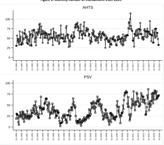
represent 98.6% of all spot fixtures (N=30,592). For this subsample, 18,194 and 12,398 fixtures concern the spot market for AHTS and PSVs, respectively. Figure 1 reports the number of monthly transactions over the period. For AHTS, it ranges from 25 (in November 2005) to 115 (in August 2010), with a monthly mean number of 56 transactions. For PSV, it ranges from 2 (in May 1997) to 86 (in December 2013), with an average at 38 transactions.
Insert Figure 1
8 For details, see https://login.ods-petrodata.com/.
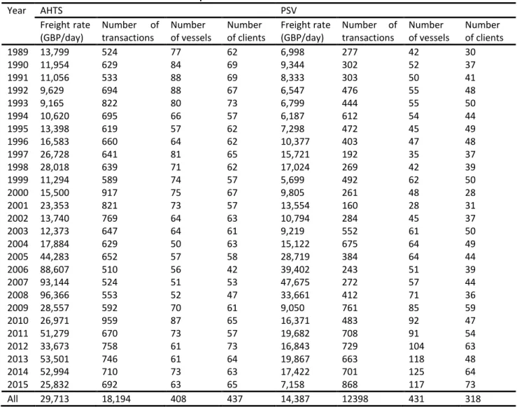
Table 1 provides some descriptive yearly statistics related to the OSV market. The average AHTS spot freight rate is twice as high (29,713 GBP/day) as the average spot rate in the PSV segment (14,387 GBP/day). We find evidence of high volatility for both vessel categories. For AHTS, the median dayrate is around half the average rate (53.9%) and the coefficient of variation is 1.25. For PSV, the ratio between the median and average dayrate is equal to 0.703 and the coefficient of variation is substantially lower (0.87). The highest monthly average dayrate is observed in 2008 for AHTS (at 96,366 GBP/day) and in 2007 for PSV (at 47,675 GBP/day).
The number of distinct vessels chartered is rather similar for both subsamples (408 for AHTS and 431 for PSV), and we note an increase in the number of transactions at the end of the period for PSV only. The number of clients (charterers) is higher on the AHTS market (437) than on the PSV market (318), but it remains rather stable over the period (with an average of 62 for AHTS and 46 for PSV). The three largest charterers are Statoil (N=1,566), ASCO (N=1,033) and Shell (N=951) for AHTS and Team (N=1,056), Shell (N=858) and ASCO (N=857) for PSV10.
Insert Table 1
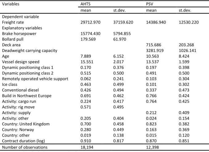
Table 2 contains the descriptive statistics for the variables selected to explain the dayrate. For AHTS, the average Brake horsepower is 15,774 and the average bollard pull is 180 tonnes. For PSV, the average deck area is 613 m² and the average deadweight carrying capacity is 2,959 tonnes. The average age of vessels is 7.9 years for AHTS and 10.5 years for PSV. The average design speed is slightly higher for AHTS (15.6 knots) than for PSV (13.5 knots). The proportion of vessels with a dynamic position system of class 2 is 51.5% for AHTS and 49.1% for PSV. AHTS are used for rig moves and cargo runs in 80% of the cases, while 97% of PSV activities are cargo-run and supply-related. Most activities are taking place in the territorial waters of the United Kingdom (70.0% for AHTS and 82.3% for PSV).
Insert Table 2
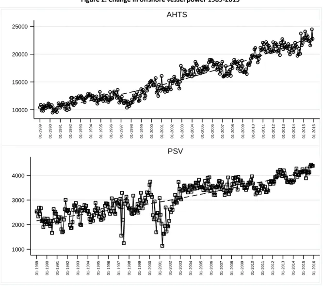
As drilling rigs have gradually become larger and are operating in remote areas further from the shore, a substantial increase in the horsepower and size of the OSV vessels has taken place as shown in Figure 2. From 1989 to 2015, the power of offshore support vessels has more than doubled. The average brake horsepower for AHTS has increased from 10,000 to nearly 24,000 BHP and the average deck area has grown from 2,000 to 4,000 m² for PSV, with an exponential trend in both cases11. This increase in power is expected to contribute to
10 Charterers are either some major international oil companies (Shell, Statoil) or logistics companies (e.g. Team
or ASCO) working on behalf of oil companies (Institute of Chartered Shipbrokers, 2011).
11 When estimating the log of power as a function of the log of time, we find an elasticity of 0.217 for brake
increased freight rates. We thus turn to an econometric framework to account for these composition effects.
Insert Figure 2
5. Empirical results
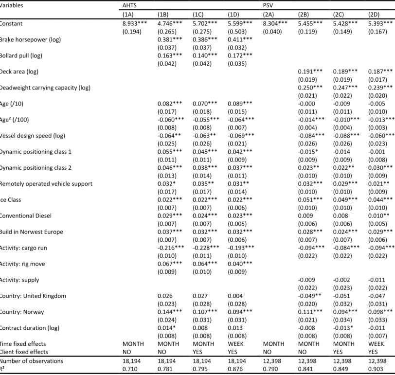
We estimate the hedonic price regressions described in section 3 for the AHTS and PSV markets on a monthly and weekly basis, respectively. In columns 1A (AHTS) and 2A (PSV) of Table 3, we only include monthly fixed effects as covariates so that the time fixed effect 𝑡 will correspond to the average score 𝐹̅𝑡. There are substantial variation in freight rates over
time since between 70% and 80% of variation in dayrates is explained by the inclusion of time dummies in the regression (R²=0.71 for AHTS, R²=0.79 for PSV).
In columns 1B and 2B, we add covariates related to vessel characteristics and contractual terms such as duration, type of activity and geographic location. Including these additional controls increases the R2 by 7.1 percentage points for the AHTS market and 5.1 percentage
points for the PSV market. Given the marginal improvement in explanatory power between specifications A and B, we test for the joint significance of vessel and contract specific variables. For models (1B) and (2B), we find values of 293.87 and 238.73 for the corresponding Wald test with p<.0001 in both cases, meaning that the covariates remain jointly significant in our regressions
Insert Table 3
For both types of vessels, most covariates are significant at conventional levels and have the expected sign12. For instance, a 1% increase in a vessel’s break horsepower leads to a 0.38%
increase in the AHTS spot freight rate. Freight rates decrease with vessel age. A 1% increase in vessel design speed, which may be seen a proxy for fuel consumption, leads to a 0.06% decrease in freight rate. Vessels equipped with dynamic positioning (either system 1 or system 2), ROV support, ice class or built in Northwest Europe are subject to a freight rate premium. When AHTS are used for cargo runs, which is not their core activity, the daily freight rate is lower. This is consistent with the observation that these vessels are not optimal for cargo runs and will only compete for such contracts during poor markets conditions.
For PSVs, a 1% increase in deck area leads to a 0.19% increase in the spot freight rate and the corresponding elasticity for the deadweight carrying capacity is 0.25%. As for AHTS, the
12 We have also estimated a model including a vessel fixed effect as well as age and age squared since age is a
time-varying explanatory variable. In that case, the increase in R² is marginal compared to (1B) and (2B) with R²=0.799 for AHTS (R²=0.795 without the vessel fixed effect) and R²=0.864 for PSV (R²=0.849 without the vessel fixed effect).
relationship between dayrates and age, speed as well as the cargo run activity is negative. The preference for DP2 systems is clear for PSVs, which is to be expected as these vessels must operate very close to the rigs during cargo handling operations. A premium is also added to the dayrate when the vessel includes ROV support and ice-class, and when the vessel was built in Northwest Europe. Both for AHTS and PSV, contract duration is not significant at the 5% level. This is perhaps to be expected given that we are dealing with a spot market with very short-term contracts.
Next, we account for time-invariant unobserved characteristics of clients (charterers). Two additional results emerge from the data (columns 1C and 2C, Table 3). First, compared to (1B) and (2B), the improvement of the fit of the regressions is really marginal since the increase in R² amounts to 1.4 percentage point for AHTS and 0.8 percentage point for PSV. One explanation is that the OSV market is near perfectly competitive. Similarly, the introduction of a client fixed effect has very little effect on the other coefficients (both in terms of sign and statistical significance) in the regression.
Finally, we re-estimate the full model with weekly instead of monthly time fixed effects (columns 1D and 2D, Table 3) to assess the impact of the choice of time unit. The results suggest that for both the AHTS and PSV segments, considering time dummies at the weekly level provides a substantially better fit to the data. Specifically, it increases the R² by a further 8.1 percentage points and 5.4 percentage points, respectively, to 0.876 for AHTS and 0.903 for PSV. This improvement in the fit of the regressions is expected since working at the weekly level allows to better pick up the volatility in dayrates compared to monthly average values.
We then run various tests to check the robustness of our estimates. First, a concern is related to a potential multicollinearity between some of the vessel characteristics. The most important correlations are between the logarithms of brake horsepower and bollard pull (0.971) for AHTS and between the logarithms of deck area and deadweight carrying capacity (0.875) for PSV. Estimates of the variance inflation factors associated to regressions 1B and 2B in Table 3 are equal to 21.5 and 19.3 for brake horsepower and bollard pull for AHTS and to 5.31 and 7.52 for deck area and deadweight carrying capacity for PSV. As variance inflation factors exceed 10 for AHTS, we re-estimated model 1B with only one indicator of power. Our results, not reported here, show that the coefficient associated to either brake horsepower or bollard pull is much higher when each covariate is introduced separately (0.511 against 0.381 for brake horsepower, 0.551 against 0.163 for bollard pull). However, controlling for both covariates does not significantly affect other estimates and the R². Second, we have checked for the presence of influential transactions. We find that residuals range between -2.9 and 2.6 for AHTS (model 1C) and -2.4 and 3.1 for AHTS (2C). Third, we implemented a test on the normality of residuals, although normality is not required to have
unbiased estimates of the coefficients in an OLS regression. For each model, we compare the kernel density of the estimated residuals with those from a comparable normal density and find that residuals are very close to a normal distribution. Finally, the Breusch-Pagan tests for heteroskedasticity lead to values equal to 754.9 for AHTS and 32.6 for PSV, with p<0.001 in both cases. This rejects the null hypothesis that the variance of the residuals is homogenous and supports our decision to report heteroskedasticity robust standard errors.
Finally, a last element is about the relevance of the way we account for time effects in our analysis. In (3), we explain 𝐹𝑖 as a function of time dummies 𝕝𝑡 so that our model is a fixed
effect specification which can be alternatively expressed as 𝐹𝑖 = 𝛿𝑡+ 𝑋𝑖𝛽 + 𝛾𝑐 + 𝜀𝑖. In doing
so, we allow the time fixed effects 𝛿𝑡 to be correlated with the other explanatory variables
introduced in the regression. An alternative specification would be to relax this endogeneity assumption and to consider instead a random model estimated using feasible Generalized Least Squares. In order to know which specification is more appropriate, we turn to the classical Hausman test (Hausman, 1978). Results for the null assumption associated to the random effect model give values of 231.5 for AHTS and 140.1 for PSV with p<0.001 in both cases, so that a model with time dummies to construct a market index is appropriate given the data at hand.
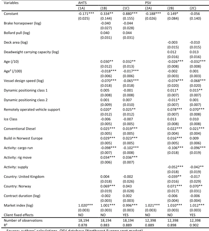
As brokers market indices have been generally used as explanatory variables in the literature explaining fixture rates (Alizadeh and Talley, 2011a,b; Köhn and Thanopoulou, 2011; Adland et al, 2016, 2017), we investigate whether our results reported in Table 3 would be significantly different if a third-party market index is used as a control instead of our time fixed effect index. The monthly models of Table 3 were thus re-estimated with the inclusion of a market index obtained from shipbroker Clarksons Platou. The index reflects brokers’ assessment of the prevailing dayrate for a particular size segment in the North Sea OSV market. We present the corresponding estimates in Table A in Appendix both for AHTS and PSV.
Our results show that the inclusion of an external market index instead of our time fixed effects has two main effects. Firstly, the explanatory power of all models is nearly identical, and the market index coefficient is close to 1.0. This suggests that the broker index dominates the models since the R² with market index as control only is around 0.9 both for AHTS and PSV. Secondly, the magnitude of the coefficients and level of significance for some vessel characteristics and contract variables change substantially. For instance, the coefficient for age is reduced from 0.082 (column 1B, Table 3) to 0.030 with the market index (column 1B, Table A). Similarly, characteristics that are known to be important, such as brake horsepower and bollard pull for AHTS, become insignificant with the marked index as control. This highlights the likely endogeneity of the external market index due to the circularity problem emphasized earlier.
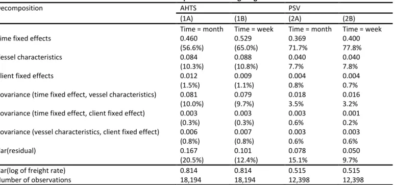
Next, we assess the respective contributions of the time fixed effects, the vessel characteristics and the client fixed effects using the variance decomposition corresponding to equation (4). Results reported in Table 4 correspond to specifications (1C) and (1D) of Table 3 for the AHTS segment and (2C) and (2D) for the PSV segment. For both markets, the contribution of the time fixed effects is the largest. When the time unit is defined at the monthly level (columns 1A and 2A), it explains 56.6% of dayrate variation for the AHTS market and 71.7% for the PSV market. The influence of vessel characteristic is more limited (10.2% for AHTS and 7.7% for PSV). By comparison, the contribution of client fixed effects in the variance decomposition is 1.5% for AHTS and 0.8% for PSV.
Insert Table 4
We find a contribution of 10.0% for the covariance term between monthly fixed effects and vessel characteristics for the AHTS market (3.5% for the PSV market). This is evidence that the time fixed effect is correlated to vessel characteristics. The contribution of the residual (20.5% for AHTS, 15.1% for PSV) is much higher than that obtained in recent empirical studies explaining freight rates from fixture data (Alizadeh and Talley, 2011a, 2011b, Adland et al., 2016, 2017). However, in these studies, the R² is near one because the market indicator is itself included as additional control in the regression. Finally, Table 4 shows that the contribution of time fixed effects increases to 65% for AHTS and 77.8% for PSV when the time unit is the week (columns 1B and 2B, Table 4).
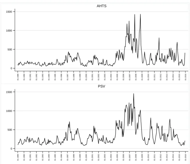
Using estimates from models (1C) and (2C) of Table 3, Figure 3 presents the AHTS and PSV estimated monthly market index over the entire period, with base 100 in January 1989. For the AHTS market, the index ranges between 100 and 500 from 1989 till 2006. Then, freight rates go up, with index values reaching nearly 1500 in mid-2008, pushed by the general increase in oil prices leading to more offshore exploration projects. At the same time, the 2007-2009 period is characterized by substantialy volatility in dayrates. After 2009 and following the mid-2008 financial crisis, the index remains essentially in the 100-500 range with an average of 257 between 2009 and 2015. Very similar results are found for the PSV market. In particular, the market index substantially increases between 2006 and 2009 and dayrates are rather volatile.
Insert Figure 3
Overall, our variance decomposition highlights the role of time when explaining dayrates. In what follows, we further attempt to investigate the estimated fixed effects denoted by 𝛿̂𝑡. In this second-stage analysis, we consider two main set of covariates. First, there may be some seasonality in dayrates over the calendar year which is picked up using calendar monthly dummies. This is likely to be the case for vessels operating in the North Sea, an area which is subject to a harsh environment in winter. We expect bad weather conditions to result in
lower demand for OSVs and therefore lower dayrates. Second, as drilling rig activity – and therefore demand for OSVs – has been shown to depend on expected oil prices (Ringlund et al, 2008), we explore the relationship between the OSV market and oil prices (spot and futures) in addition to more direct measures of activity such as oil production.
For the presentation, let 𝕝𝑚 be a set of dummies associated to calendar months with 𝑚 = 1 for January and 𝑚 = 12 for December. We denote by 𝑄𝑡 the combined oil production from
the United Kingdom and Norway expressed in million barrels per day and 𝑃𝑡 the Brent oil
spot price expressed in US dollar per barrel13. We also consider Brent futures prices 𝑃 𝑡
𝑓
(2 months and 12 months maturity) and the slope of the Brent forward curve defined as 𝑃𝑡𝑓− 𝑃𝑡. We turn to a weighted least-square regression with the monthly number of fixtures as
weight to explain the estimate time fixed effect 𝛿̂𝑡14:
𝛿̂𝑡 = ∑12𝑚=2𝜗𝑚∗ 𝕝𝑚+ 𝜇 ln 𝑄𝑡+ 𝜋 ln 𝑃𝑡+ 𝜁𝑡 (5)
where 𝜗𝑚, 𝜇 and 𝜋 are parameters to estimate. We rely on a bootstrap procedure to obtain
standard errors for 𝜗𝑚, 𝜇 and 𝜋. Using 250 random samples of fixtures drawn in the full
sample of transactions, we re-estimate in two steps both equations (3) and (5)15. We present
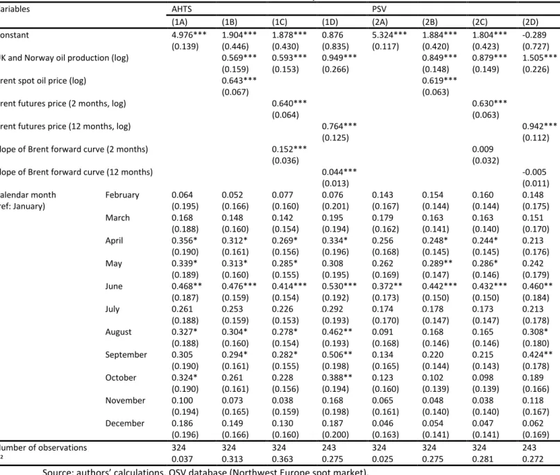
the second-stage estimates in Table 5.
Insert Table 5
In columns (1A) and (2A), we only include the calendar month effects as covariates. Our results suggest that there is some seasonality in the OSV market. For the AHTS market, the estimated monthly fixed effect is much higher from April to October (and especially in June) compared to November till March. The lowest coefficients are those of the reference category January and the month of February, which is typically a period of strong winds and high waves in the North Sea. Seasonality is less pronounced in the PSV market, but again our results show larger values for the calendar dummies from April till June when vessels operate in benign weather conditions. At the same time, we note that the contribution of the calendar dummies to the R² remains relatively low (around 3%).
As shown in Table 5, we find a positive correlation between our monthly index and both oil production in the North Sea and the Brent Oil Price (columns 1B and 2B). The contribution to the R² of these two covariates is 27.6 percentage points for the AHTS market and 25
13 For these additional data, sources are EIA for Norway and United Kingdom oil production and Datastream for
Brent oil prices. Although we acknowledge that both oil production and oil price are strongly interrelated, we nonetheless choose to include both covariates in the regression.
14 We turn to a weighted least-square regression because the dependent variable 𝛿̂
𝑡 is obtained from the
first-stage linear regression (3).
15 We have checked the stationarity of the series of monthly fixed effects 𝛿̂
𝑡 using a Dickey-Fuller test. Both for
percentage points for the PSV market. In both cases, elasticities of oil price and oil production are around 0.5-0.6 for AHTS vessels and 0.6-0.8 for PSV vessels. However, implementation of a Shapley decomposition (Huettner and Sunder, 2012) shows that the contribution to the R² is four times higher (80% compared to 20%) for the oil price than for oil production. As expected, these results suggest that the level of activity in the world oil market is an influential driver of the OSV freight market. Substituting spot prices with short-term oil futures prices and adding the slope of the oil forward curve as a covariate (specifications 1C and 2C) adds some explanatory power to the model whereas longer-term futures prices do not (specifications 1D and 2D). This suggests that the OSV spot market is more susceptible to changes in short-run oil market sentiment and points to the possibility of spillover effects between related markets in the energy complex. Spillover effects and transmission mechanisms between shipping markets have been considered in the recent literature on freight derivatives (Alexandridis et al, 2017). In related work, Papapostolou et. al. (2014) consider the impact of investor sentiment on ship investment returns. For instance, we expect that market sentiment and contract pricing in the rig market will impact sentiment and pricing in the OSV chartering market. Having an objective market index is key to be able to evaluate such transmission mechanisms and our work represents a first step towards this line of research.
6. Concluding remarks
In this paper, we have developed and applied a methodology that enables us to extract a freight market index from raw fixture data where we control for vessel and contract-specific variables as well as charterer fixed effects. Compared to indices based on the expert opinion of shipbrokers, the main advantage of our approach is its proper adjustment for heterogeneity in the underlying raw data, particularly when there are structural shifts in the technical specifications and composition of the fleet and market players. We have also shown that the inclusion of brokers’ market indices as a control variable substantially affects the estimated coefficients of vessel and contract-specific factors, which confirms that these indices pick up composition effects in addition to market conditions. This is an important finding for all future research based on micro fixture data and positions our proposed methodology as one way to avoid this endogeneity problem.
Our empirical results with regards to the OSV segment can be summarized as follows. Firstly, around 70%-80% of variation in OSV dayrates is explained by time fixed effects. Secondly, most vessel characteristics have the expected sign in the hedonic price regression and spot freight rates increase significantly with the power and capacity of OSVs. Thirdly, the contribution of charterer fixed effects is limited in terms of magnitude, which may be related to the competitive nature of the OSV markets with charterers being price takers. Fourthly, both for the AHTS and PSV segments, the market indices are rather volatile and characterized by some seasonality with higher values during Spring and Summer. Finally, our
second-stage estimates of the determinants of the market index suggest that oil production, oil prices and the slope of the oil forward curve significantly affects OSV dayrates.
It is worth noting that we do not suggest that our market index is better than indices provided by shipbrokers that are published on a regular basis. Indeed, we acknowledge that our data-driven approach may have drawbacks compared to the human expertise which forms the basis of all current market indices in shipping. In particular, we are reliant on having observations in each time step (which is one week or one month in our context) in order to estimate time fixed effects. This means that we are, in general, unable to estimate indices at a higher frequency than one week in most shipping and offshore markets as there would not be enough transactions, particularly if we disaggregate to the regional or route level.
As a related point, our information set consists only of realized and public transactions, which do not necessarily give the full picture. While the offshore market considered here is highly transparent compared to most other areas of shipping, we cannot be assured that all fixtures are included. Moreover, knowledge of bids and offers in ongoing negotiations, even if they may ultimately fail, will give the shipbroker a more continuous information on the appropriate market level than the discrete observations of realized transactions in our dataset.
Future research within this topic should consider whether the methodology can be extended to deduce the market index at a higher frequency and from a broader information set. It would also be useful to extend the empirical results to other traditional deep-sea shipping segments, provided the availability and coverage of the raw fixture data is adequate. Developing consistent spot market indices across the OSV and rig markets would also enable time-series analysis of the transmission mechanisms between these related markets. However, this would require a similar empirical analysis of rig contracts, a market that is substantially less liquid and perhaps even more heterogeneous than that for the chartering of OSVs.
Appendix
References
Aas, B., Halskau, Ø. and Wallace, S.W. (2009), The role of supply vessels in offshore logistics,
Maritime Economics and Logistics, vol. 11, pp. 302-325.
Adland, R., Alger, H., Banyte, J. and Jia, H. (2017), Does fuel efficiency pay? Empirical evidence from the drybulk timecharter market revisited, Transportation Research Part A, vol. 95, pp. 1-12.
Adland, R., Cariou, P., and Wolff, F.C. (2016), The influence of charterers and owners on bulk shipping freight rates, Transportation Research Part E: Logistics and Transportation Review, vol. 86, pp. 69-82.
Adland, R. and Cullinane, K. (2006), The non-linear dynamics of spot freight rates in tanker markets, Transportation Research Part E, vol. 42, pp. 211-24.
Adland, R., Jia, H., and Lu, J. (2008), Price dynamics in the market for Liquid Petroleum Gas transport, Energy Economics, vol. 30, pp. 818-828.
Agnolucci, P., Smith, T. and Rehmatullah, N. (2014), Energy efficiency and time charter rates: Energy efficiency savings recovered by ship owners in the Panamax market, Transportation
Research Part A, vol. 66, pp. 173-184.
Alexandridis, G., Sahoo, S., and Visvikis, I. (2017), Economic information transmissions and liquidity between shipping markets: New evidence from freight derivatives. Transportation
Research Part E: Logistics and Transportation Review, vol. 98, pp. 82-104.
Alizadeh A.H. and Talley, W.K. (2011a), Vessel and voyage determinants of tanker freight rates and contract times, Transport Policy, vol. 18, pp. 665-675.
Alizadeh, A.H., and Talley, W.K. (2011b), Microeconomic determinants of dry bulk shipping freight rates and contract times, Transportation, vol. 38, pp. 561-579.
Baltic Exchange, (2016), Manual for panelists, www.balticexchange.com.
Bates, T.H. (1969), A linear regression model of ocean tramp rates, Transportation Research, vol. 3, pp. 377-395.
Berg-Andreassen, J.A. (1996), Some properties of international maritime statistics, Maritime
Bjerksund, P. and Ekern, S. (1995), Contingent claims evaluation for mean-reverting cash flows in shipping, in Trigeorgis, L. (ed.), Real options in capital investments, models,
strategies, and applications, Praeger, Westport.
Clarkson Research, 2016, Shipping Intelligence Network database, www.clarksons.net. Fernandez Cuesta, E., Andersson, H., Fagerholt, K. and Laporte, G. (2017), Vessel routing with pickups and deliveries: An application to the supply of offshore oil platforms,
Computers and Operations Research, vol. 79, pp. 140-147.
Franses, P. and Veenstra, A. (1997), A co-integration approach to forecasting freight rates in the dry bulk shipping sector, Transportation Research, vol. 31, pp. 447-458.
Gobillon, L. and Wolff F-C. (2016), Evaluating the Law of one Price Using Micro Panel Data: The Case of the French Fish Market, American Journal of Agricultural Economics, vol. 98(1), pp 134-153
Hausman, J.A. (1978), Specification tests in econometrics, Econometrica, vol. 46, pp. 1251-1271.
Institute of Chartered Shipbrokers (2011), Offshore Support Industry. Institute of Chartered Shipbrokers: London, UK.
Huettner, F. and Sunder, M. (2012), Axiomatic arguments for decomposing goodness of fit according to Shapley and Owen values, Electronic Journal of Statistics, vol. 6, pp. 1239-1250. Kaiser, M.J. (2015), Offshore Service Vessel activity forecast and regulatory modeling in the U.S. Gulf of Mexico, 2012–2017, Marine Policy, vol. 57, pp. 132-146.
Kavussanos, M. G. (1996), Comparisons of volatility in the dry-cargo ship sector: Spot versus time charters, and smaller versus larger vessels, Journal of Transport economics and Policy, vol. 30, pp. 67-82.
Kavussanos, M. G., and Alizadeh, A. H. (2001), Seasonality patterns in dry bulk shipping spot and time charter freight rates, Transportation Research Part E: Logistics and Transportation
Review, vol. 37, pp. 443-467.
Köhn, S. and Thanopoulou, H. (2011), A GAM Assessment of quality premia in the drybulk timecharter market, Transportation Research Part E, vol. 47, pp. 709-721.
Nomikos, N. and Kavussanos, M. (2000), Futures hedging when the structure of the underlying asset changes: The case of the BIFFEX contract, Journal of Futures Markets, vol. 20, pp. 775-801.
Papapostolou, N.C., Nomikos, N.K., Pouliasis, P.K. and Kyriakou, I. (2014), Investor sentiment for real assets: The case of dry bulk shipping market, Review of Finance, vol. 18, pp. 1507-1539.
Poblacion, J. (2015), The stochastic seasonal behavior of freight rate dynamics, Maritime
Economics and Logistics, vol. 17, pp. 142-162.
Población, J. (2017), Are recent tanker freight rates stationary? Maritime Economics and
Logistics, forthcoming. doi:10.1057/mel.2016.7
Ringlund, G.B., Rosendahl. K.E. and Skjerpen, T. (2008), Does oilrig activity react to oil price changes? An empirical investigation, Energy Economics, vol. 30, pp. 371-396.
Rosen, S. (1974), Hedonic prices and implicit markets: Product differentiation in pure competition, Journal of Political Economy, vol. 82, pp. 34-55.
Shimojo, T. (1979), Economic analysis of shipping freights, Kobe University, Kobe.
Tamvakis, M. N. (1995), An investigation into the existence of a two-tier spot freight market for crude oil tankers, Maritime Policy and Management, vol. 22, pp. 81-90.
Tamvakis, M. N. and Thanopoulou, H. A. (2000), Does quality pay? The case of the dry bulk market, Transportation Research Part E, vol. 36, pp. 297-307.
Triplett, J. (2006), Handbook on hedonic indexes and quality adjustments in price indexes, OECD Publishing: Paris.
Tvedt, J., (1997), Valuation of VLCCs under income uncertainty, Maritime Policy and
Management, vol. 24, pp. 159-174.
Veenstra, A., and van Dalen, J. (2008), Price indices for ocean charter contracts, In, The Second International Index Measures Congress, Washington, Digital proceedings.
Figure 1. Monthly number of transactions 1989-2015
Source: authors’ calculations, OSV database.
Note: the sample is restricted to the North Sea spot market.
0 25 50 75 100 M o n th ly n u m b e r o f tr a n s a c ti o n s 0 1 -1 9 8 9 0 1 -1 9 9 0 0 1 -1 9 9 1 0 1 -1 9 9 2 0 1 -1 9 9 3 0 1 -1 9 9 4 0 1 -1 9 9 5 0 1 -1 9 9 6 0 1 -1 9 9 7 0 1 -1 9 9 8 0 1 -1 9 9 9 0 1 -2 0 0 0 0 1 -2 0 0 1 0 1 -2 0 0 2 0 1 -2 0 0 3 0 1 -2 0 0 4 0 1 -2 0 0 5 0 1 -2 0 0 6 0 1 -2 0 0 7 0 1 -2 0 0 8 0 1 -2 0 0 9 0 1 -2 0 1 0 0 1 -2 0 1 1 0 1 -2 0 1 2 0 1 -2 0 1 3 0 1 -2 0 1 4 0 1 -2 0 1 5 0 1 -2 0 1 6 AHTS 0 25 50 75 100 M o n th ly n u m b e r o f tr a n s a c ti o n s 0 1 -1 9 8 9 0 1 -1 9 9 0 0 1 -1 9 9 1 0 1 -1 9 9 2 0 1 -1 9 9 3 0 1 -1 9 9 4 0 1 -1 9 9 5 0 1 -1 9 9 6 0 1 -1 9 9 7 0 1 -1 9 9 8 0 1 -1 9 9 9 0 1 -2 0 0 0 0 1 -2 0 0 1 0 1 -2 0 0 2 0 1 -2 0 0 3 0 1 -2 0 0 4 0 1 -2 0 0 5 0 1 -2 0 0 6 0 1 -2 0 0 7 0 1 -2 0 0 8 0 1 -2 0 0 9 0 1 -2 0 1 0 0 1 -2 0 1 1 0 1 -2 0 1 2 0 1 -2 0 1 3 0 1 -2 0 1 4 0 1 -2 0 1 5 0 1 -2 0 1 6 PSV
Figure 2. Change in offshore vessel power 1989-2015
Source: authors’ calculations, OSV database (Northwest Europe spot market).
10000 15000 20000 25000 A v e ra g e b ra k e h o rs e p o w e r 0 1 -1 9 8 9 0 1 -1 9 9 0 0 1 -1 9 9 1 0 1 -1 9 9 2 0 1 -1 9 9 3 0 1 -1 9 9 4 0 1 -1 9 9 5 0 1 -1 9 9 6 0 1 -1 9 9 7 0 1 -1 9 9 8 0 1 -1 9 9 9 0 1 -2 0 0 0 0 1 -2 0 0 1 0 1 -2 0 0 2 0 1 -2 0 0 3 0 1 -2 0 0 4 0 1 -2 0 0 5 0 1 -2 0 0 6 0 1 -2 0 0 7 0 1 -2 0 0 8 0 1 -2 0 0 9 0 1 -2 0 1 0 0 1 -2 0 1 1 0 1 -2 0 1 2 0 1 -2 0 1 3 0 1 -2 0 1 4 0 1 -2 0 1 5 0 1 -2 0 1 6 AHTS 1000 2000 3000 4000 A v e ra g e d e c k a re a 0 1 -1 9 8 9 0 1 -1 9 9 0 0 1 -1 9 9 1 0 1 -1 9 9 2 0 1 -1 9 9 3 0 1 -1 9 9 4 0 1 -1 9 9 5 0 1 -1 9 9 6 0 1 -1 9 9 7 0 1 -1 9 9 8 0 1 -1 9 9 9 0 1 -2 0 0 0 0 1 -2 0 0 1 0 1 -2 0 0 2 0 1 -2 0 0 3 0 1 -2 0 0 4 0 1 -2 0 0 5 0 1 -2 0 0 6 0 1 -2 0 0 7 0 1 -2 0 0 8 0 1 -2 0 0 9 0 1 -2 0 1 0 0 1 -2 0 1 1 0 1 -2 0 1 2 0 1 -2 0 1 3 0 1 -2 0 1 4 0 1 -2 0 1 5 0 1 -2 0 1 6 PSV
Figure 3. Estimated market indices of the log freight rate
Source: authors’ calculations, OSV database (Northwest Europe spot market).
Note: the estimated indices are calculated using the monthly fixed effects obtained from models (1C) and (2C) of Table 3 for AHTS and PSV, respectively. The indices are set to 100 in January 1989.
0 500 1000 1500 Ma rk e t in d e x 0 1 -1 9 8 9 0 1 -1 9 9 0 0 1 -1 9 9 1 0 1 -1 9 9 2 0 1 -1 9 9 3 0 1 -1 9 9 4 0 1 -1 9 9 5 0 1 -1 9 9 6 0 1 -1 9 9 7 0 1 -1 9 9 8 0 1 -1 9 9 9 0 1 -2 0 0 0 0 1 -2 0 0 1 0 1 -2 0 0 2 0 1 -2 0 0 3 0 1 -2 0 0 4 0 1 -2 0 0 5 0 1 -2 0 0 6 0 1 -2 0 0 7 0 1 -2 0 0 8 0 1 -2 0 0 9 0 1 -2 0 1 0 0 1 -2 0 1 1 0 1 -2 0 1 2 0 1 -2 0 1 3 0 1 -2 0 1 4 0 1 -2 0 1 5 0 1 -2 0 1 6 AHTS 0 500 1000 1500 Ma rk e t in d e x 0 1 -1 9 8 9 0 1 -1 9 9 0 0 1 -1 9 9 1 0 1 -1 9 9 2 0 1 -1 9 9 3 0 1 -1 9 9 4 0 1 -1 9 9 5 0 1 -1 9 9 6 0 1 -1 9 9 7 0 1 -1 9 9 8 0 1 -1 9 9 9 0 1 -2 0 0 0 0 1 -2 0 0 1 0 1 -2 0 0 2 0 1 -2 0 0 3 0 1 -2 0 0 4 0 1 -2 0 0 5 0 1 -2 0 0 6 0 1 -2 0 0 7 0 1 -2 0 0 8 0 1 -2 0 0 9 0 1 -2 0 1 0 0 1 -2 0 1 1 0 1 -2 0 1 2 0 1 -2 0 1 3 0 1 -2 0 1 4 0 1 -2 0 1 5 0 1 -2 0 1 6 PSV
Table 1. Description of the OSV market 1989-2015 Year AHTS PSV Freight rate (GBP/day) Number of transactions Number of vessels Number of clients Freight rate (GBP/day) Number of transactions Number of vessels Number of clients 1989 13,799 524 77 62 6,998 277 42 30 1990 11,954 629 84 69 9,344 302 52 37 1991 11,056 533 88 69 8,333 303 50 41 1992 9,629 694 88 67 6,547 476 55 48 1993 9,165 822 80 73 6,799 444 55 50 1994 10,620 695 66 57 6,187 612 54 44 1995 13,398 619 57 62 7,298 472 45 49 1996 16,583 660 64 62 10,377 403 47 48 1997 26,728 641 81 65 15,721 192 35 37 1998 28,018 639 71 62 17,024 269 42 39 1999 11,294 589 74 57 5,699 492 62 50 2000 15,500 917 75 67 9,805 261 48 28 2001 23,353 821 73 57 13,554 160 28 31 2002 13,740 769 64 63 10,794 284 45 37 2003 12,373 647 64 61 9,219 552 61 50 2004 17,884 629 50 63 15,122 675 64 49 2005 44,283 652 57 58 28,719 384 64 44 2006 88,607 510 56 42 39,402 243 51 39 2007 93,144 524 51 53 47,675 272 57 44 2008 96,366 553 52 47 33,661 412 71 36 2009 28,557 592 70 61 9,050 761 85 59 2010 26,971 959 87 65 16,371 483 92 47 2011 51,279 670 73 57 19,682 708 91 54 2012 33,673 758 61 73 16,843 729 104 63 2013 53,501 746 61 64 19,867 663 118 48 2014 52,994 710 73 63 17,422 701 125 64 2015 25,832 692 63 65 7,158 868 117 73 All 29,713 18,194 408 437 14,387 12398 431 318
Source: authors’ calculations, OSV database.
Table 2. Description of PSV fixtures 1989-2015
Variables AHTS PSV
mean st.dev. mean st.dev.
Dependent variable Freight rate 29712.970 37159.620 14386.940 12530.220 Explanatory variables Brake horsepower 15774.430 5794.855 Bollard pull 179.569 61.970 Deck area 715.686 203.268
Deadweight carrying capacity 3281.919 1026.141
Age 7.889 6.152 10.563 8.424
Vessel design speed 15.551 2.017 13.537 1.599
Dynamic positioning class 1 0.170 0.376 0.197 0.398
Dynamic positioning class 2 0.515 0.500 0.491 0.500
Remotely operated vehicle support 0.062 0.241 0.103 0.304
Ice class 0.463 0.499 0.101 0.302
Conventional diesel 0.426 0.494 0.337 0.473
Build in Northwest Europe 0.691 0.462 0.766 0.424
Activity: cargo run 0.224 0.417 0.764 0.425
Activity: rig move 0.571 0.495
Activity: supply 0.212 0.409
Activity: other 0.205 0.404 0.024 0.154
Country: United Kingdom 0.700 0.458 0.823 0.382
Country: Norway 0.280 0.449 0.163 0.369
Country: other 0.019 0.138 0.015 0.120
Contract duration (log) 0.910 0.817 0.870 0.851
Number of observations 18,194 12,398
Source: authors’ calculations, OSV database.
Table 3. Estimates of the log of freight rate
Variables AHTS PSV
(1A) (1B) (1C) (1D) (2A) (2B) (2C) (2D) Constant 8.933*** 4.746*** 5.702*** 5.599*** 8.304*** 5.455*** 5.428*** 5.393***
(0.194) (0.265) (0.275) (0.503) (0.040) (0.119) (0.149) (0.167) Brake horsepower (log) 0.381*** 0.386*** 0.411***
(0.037) (0.037) (0.032) Bollard pull (log) 0.163*** 0.140*** 0.172***
(0.042) (0.042) (0.035)
Deck area (log) 0.191*** 0.189*** 0.187***
(0.019) (0.019) (0.017) Deadweight carrying capacity (log) 0.250*** 0.247*** 0.239***
(0.021) (0.022) (0.020) Age (/10) 0.082*** 0.070*** 0.089*** -0.000 -0.009 -0.005
(0.017) (0.018) (0.015) (0.011) (0.011) (0.010) Age² (/100) -0.060*** -0.055*** -0.064*** -0.014*** -0.010*** -0.013***
(0.008) (0.008) (0.007) (0.004) (0.004) (0.003) Vessel design speed (log) -0.064** -0.063** -0.069*** -0.084*** -0.088*** -0.060***
(0.025) (0.026) (0.021) (0.026) (0.026) (0.023) Dynamic positioning class 1 0.055*** 0.045*** 0.042*** -0.015* -0.014 -0.001
(0.011) (0.011) (0.009) (0.009) (0.009) (0.008) Dynamic positioning class 2 0.046*** 0.038*** 0.037*** 0.023** 0.022** 0.030***
(0.013) (0.014) (0.011) (0.010) (0.010) (0.009) Remotely operated vehicle support 0.032* 0.035** 0.031** 0.032*** 0.029*** 0.021**
(0.017) (0.017) (0.014) (0.010) (0.010) (0.009) Ice Class 0.022*** 0.022*** 0.022*** 0.051*** 0.049*** 0.044***
(0.007) (0.007) (0.006) (0.010) (0.010) (0.010) Conventional Diesel 0.029*** 0.024*** 0.023*** 0.009 0.008 0.010**
(0.007) (0.007) (0.005) (0.006) (0.006) (0.005) Build in Norwest Europe 0.037*** 0.032*** 0.032*** 0.028*** 0.024*** 0.029***
(0.007) (0.007) (0.006) (0.007) (0.007) (0.006) Activity: cargo run -0.216*** -0.228*** -0.193*** -0.094*** -0.084*** -0.094***
(0.010) (0.011) (0.010) (0.022) (0.022) (0.022) Activity: rig move 0.067*** 0.064*** 0.040***
(0.009) (0.010) (0.009)
Activity: supply -0.009 -0.002 -0.011
(0.022) (0.023) (0.022) Country: United Kingdom 0.026 0.027 0.004 -0.049** -0.051 -0.047
(0.023) (0.028) (0.028) (0.020) (0.032) (0.031) Country: Norway 0.144*** 0.107*** 0.094*** 0.111*** 0.094*** 0.098***
(0.024) (0.031) (0.031) (0.021) (0.034) (0.033) Contract duration (log) 0.014* 0.008 0.013 -0.008 -0.013* -0.011
(0.008) (0.008) (0.008) (0.008) (0.008) (0.007) Time fixed effects MONTH MONTH MONTH WEEK MONTH MONTH MONTH WEEK Client fixed effects NO NO YES YES NO NO YES YES Number of observations 18,194 18,194 18,194 18,194 12,398 12,398 12,398 12,398 R² 0.710 0.781 0.795 0.876 0.790 0.841 0.849 0.903
Source: authors’ calculations, OSV database (Northwest Europe spot market).
Note: estimates from linear regression models, with robust standard errors in parentheses. Significance levels are 1% (***), 5% (**) and 10% (*).
Table 4. Variance decomposition of the log freight rate
Decomposition AHTS PSV
(1A) (1B) (2A) (2B)
Time = month Time = week Time = month Time = week
Time fixed effects 0.460 0.529 0.369 0.400
(56.6%) (65.0%) 71.7% 77.8%
Vessel characteristics 0.084 0.088 0.040 0.040
(10.3%) (10.8%) 7.7% 7.8%
Client fixed effects 0.012 0.009 0.004 0.004
(1.5%) (1.1%) 0.8% 0.7%
Covariance (time fixed effect, vessel characteristics) 0.081 0.079 0.018 0.016
(10.0%) (9.7%) 3.5% 3.2%
Covariance (time fixed effect, client fixed effect) 0.003 0.003 0.003 0.001
(0.3%) (0.3%) 0.6% 0.2%
Covariance (vessel characteristics, client fixed effect) 0.006 0.007 0.003 0.003
(0.8%) (0.8%) 0.6% 0.6%
Var(residual) 0.167 0.101 0.078 0.050
(20.5%) (12.4%) 15.1% 9.7%
Var(log of freight rate) 0.814 0.814 0.515 0.515
Number of observations 18,194 18,194 12,398 12,398
Source: authors’ calculations, OSV database (Northwest Europe spot market).
Note: the variance decompositions (1A) and (1B) correspond to models (1C) and (1D) in Table 3, the variance decompositions (2A) and (2B) correspond to models (2C) and (2D) in Table 3.