Causes of health expenditure growth : the predominance of changes in medical practices over population ageing

(1)

Causes of Health

Expenditure Growth: the

Predominance of Changes

in Medical Practices Over

Population Ageing

Brigitte DORMONT

*

_{and Hélène HUBER}

†123

ABSTRACT. – On the basis of French individual data, this paper compares

the effects of demographic change, changes in morbidity and changes in practices on the growth in health expenditures that occurred between 1992 and 2000. Micro simulations show that the rise in expenditures due to ageing is relatively small and that the impact of changes in practices is 3.8 times larger. Furthermore, changes in morbidity induce savings which more than offset the increase in spending due to population ageing.

Les causes de la croissance des dépenses de santé : la

prédo-minance des changements de pratiques sur le vieillissement

RÉSUMÉ. – Cet article compare, sur données individuelles françaises,

les effets sur la croissance des dépenses de santé, observée entre 1992 et 2000, des changements démographiques, des changements de pratiques médicales et des changements de morbidité. Des micro-simulations montrent que la croissance des dépenses attribuable au vieillissement est relativement faible. L’impact des changements de pratique est 3.8 fois plus élevé. En outre, les changements de morbidité induisent des économies qui compensent largement l’effet du vieillissement.

We are grateful for helpful comments from Chantal Cases (IRDES), Michel Lubrano (University of Marseille), Michel Grignon (McMaster University), Dominique Polton (CNAMTS) and Catherine Sermet (IRDES). We also thank the participants of the Four-geaud, LEGOS, INED and DELTA seminars in Paris and of the IEMS seminar (Univer-sity of Lausanne) as well as the participants of the third Journées Louis-André Gérard-Varet (Marseille) for useful comments. We also wish to thank two anonymous referees whose comments helped us to improve the paper. Any errors are our responsibility.

*_{B. D}_ORMONT_{: LEGOS, Université Paris Dauphine, Place du Maréchal de Lattre de}

Tassigny, 75016 Paris, France and IEMS Lausanne, Switzerland - brigitte.dormont@ dauphine.fr

†_{H. H}_UBER_{: IRDES, Paris and EconomiX, Université Paris 10, 200, avenue de la}

(2)

1 Introduction

Population ageing is often considered a major determinant of the future evolu-tion of health care expenditures. Indeed, individual health care expenditure is an increasing function of age. As life expectancy keeps improving in developed coun-tries, the growing proportion of elderly people should lead mechanically to accel-erated growth of total health care expenditures. The consequences of ageing are addressed by numerous macro and micro-economic papers. At the macro-economic level, the vast majority of studies fi nd out that the age structure of a country is not signifi cant in a regression explaining the level of total health care expenditures, whereas factors like GDP or level of education are highly signifi cant (Bac et al., 2002; Gerdtham et al., 1992, 1998; Getzen, 1992; Hitiris et al., 1992; Leu, 1986; O’Connell, 1996; OECD, 1987). At the individual level, micro-economic studies also show that ageing (represented by the individual’s calendar age) has a negli-gible infl uence on individual health care expenditures, when proximity to death is taken into account (Zweifel et al., 1999; Seshamani et al., 2004a and 2004b).

According to Zweifel et al. (1999), the correlation observed between age and health care expenditures is spurious: it results from the fact that the probability of

death increases with age, associated with the high cost of dying1_{. According to this}

analysis, individual health care expenditures should depend exclusively on proxim-ity to death, and not on age. These fi ndings are likely to explain the small impact of ageing at the macro level. As stated by Stearns and Norton (2004), predictions failing to take proximity to death into account might even be misleading, resulting in an overstated effect of ageing on future health expenditures.

The effect of ageing on health care expenditures is usually thought to result from the combination of two phenomena: population ageing and the fact that health care expenditures increase with age. Until recently, most projections of future health care expenditures simulated the impact of ageing by simply applying demographic projections to the observed expenditure profi le.

However, changes in health care expenditure level also depend on changes over time in the profi le by age group. Figure 1 presents these profi les computed for the years 1992 and 2000. Age group 0 corresponds to people age 0-9, age group 10 to people age 10-19, and so on, until age group 70, which is related to people age 70 and over. As expected, expenditures increase with age. The main feature of the graph, however, is that a sizeable upward drift of the profi le is observed between 1992 and 2000. This drift is linked to changes in patients’ behaviour and in physi-cians’ practices, as well as to technological progress. As we will show, it cannot be linked to changes in the health condition of patients, since our data reveal that they are in better shape over time.

Consequently, the increase in total health care expenditures in France can be

explained by three distinct factors: the pure demographic effect (namely, the

increase in the number and proportion of elderly people, given that health

expen-diture is an increasing function of age); changes in morbidity at a given age;

changes in practices, for a given age and morbidity level. This can be linked to

1. For Medicare, payments per person-year for decedents are 7 times larger than for survivors; in France, the corresponding coeffi cient is equal to 5.

(3)

technological progress and changes in behaviour. The aim of this paper is basically to disentangle, evaluate and interpret the respective effects of these three factors.

Our data is a representative sample of 3,441 and 5,003 French individuals observed in 1992 and 2000. We use microsimulation techniques to evaluate retro-spectively the components of the drift observed between 1992 and 2000 in the age profi le of health expenditures. Our results show that changes in morbidity induce a downward drift of the health care expenditures profi le, whereas the drift due to changes in practices is upward and sizeable.

Once we have evaluated the respective infl uences of changes in morbidity and changes in practices at the microeconomic level, we apply our results to the age structure of the French population to compare the aggregate effects of demographic change and profi le drifts for the period 1992-2000. At the macroeconomic level, the rise in health care expenditures due to demographic change is very small, in comparison with the effects of changes in practices. For total expenditures, we fi nd that the impact of changes in practices is 3.8 times larger than the rise in health care expenditures due to changes in the age structure of the population.

In comparison with studies that concentrate on time to death (Zweifel et al., 1999; Seshamani et al., 2004a et 2004b), our database presents the advantage of providing information not only about “death risk”, which is an indicator of death proximity, but also about several other morbidity indicators. Furthermore, rather than studying only hospital expenditures, like Seshamani et al. or aggre-gate individual expenditures, like Zweifel et al., our dataset allows us to study the different components of individual health care expenditures: home and offi ce physician visits, pharmaceutical expenditures submitted to reimbursement, and hospital expenditures. This detailed analysis allows us to take differences between these various kinds of expenditures into account. For example, pharma-ceutical and hospital costs are much infl uenced by technological progress, unlike physician visits.

FIGURE 1

Average individual health care expenditures by age group, years 1992 and 2000

(4)

The paper is organized as follows. In the next section, we present the basic fea-tures of the data and discuss access to care for the elderly in the French health care system. Then, we study the relation between morbidity and age (section 3). The empirical approach is presented in section 4. The microeconometric results are presented in section 5. Section 6 compares the effects of ageing and changes in practices at the macro level. Section 7 concludes.

2 The Data

2.1 The French Health Care System

The French health insurance system is public and universal. About 99% of the population is covered, without age restriction: coverage is continuous over the entire life span. For the period under study, the insurance system grants unlimited access to care, without frequency restrictions. This system covers almost 100 % of hospital care expenditures and 70% of ambulatory care expenditures. A complementary insur-ance can be subscribed. It may result from a decision of the individual, but is more often provided by the employer. 80% of the population has subscribed a comple-mentary insurance, which covers the remaining 30% of the individual ambulatory care expenditures. Notice that in France specialist consultations mostly take place in ambulatory care and not within hospital. Ambulatory care coverage entails

pharma-ceutical expenditures2_{. In France, the overall value of drug prescriptions is growing}

rapidly because of the rising prices of innovations newly allowed on the market. On the whole, whereas the number of physician visits increased by 18% between 1992 and 2000, pharmaceutical expenditures increased by 59% (IRDES, 2002).

Thanks to their coverage, French elderly do not face fi nancial constraints which could limit their access to health care. In addition, since they have been well covered during their whole life before turning 65, there is no reason why health care expendi-tures should rise at this age (this rise can indeed be observed in the US, where people can delay care until they become eligible for Medicare). Being continuous over the lifetime, coverage is thus unlikely to infl uence the profi le of health expenditures by age group.

A characteristic of the period we are interested in is the modifi cation of the medical practices, notably concerning the aged. For example, medical recommendations for preventing hypercholesterolaemia have been recently extended to very old ages in France. In the same way, the use of surgical treatment of cataract changed dramati-cally for people aged 75-84 in France: the proportion of surgical treatment rose from 40 % to 55 % between 1993 and 1998 (Baubeau et al., 2001). Another example is the increasing use of angioplasty for the treatment of Acute Myocardial Infarction. In France, the proportion of treatment by angioplasty rose from 9.6 % in 1993 to 22 % in 2001 for people aged 75-84 (Oberlin et al., 2004) . On the demand side, changing

2. This contrasts strongly with other systems, such as Medicare in the US or public coverage that pre-vails in many provinces of Canada. In 2000, for instance, Medicare in the US did not cover medica-tion when it was not prescribed in hospital.

(5)

preferences towards a better well-being of the elderly can explain this increasing use of innovative procedures. On the supply side, technological progress leads to better outcomes and safety which allow the extension of innovative procedures to older people. This might indeed lead to higher costs, but to considerably better well-being for the elderly.

2.2 The Dataset

We make use of a micro-economic data set concerning 3441 insured French citi-zens for the year 1992 and 5003 for the year 2000. This data set results from a survey

(SPS, i.e. Santé Protection Sociale) conducted by IRDES3_{on a subsample drawn}

from administrative data4_{provided by the French public health insurance, which}

records every health expenditure submitted to reimbursement by subscribers (sala-ried workers, retired sala(sala-ried workers, and their family).

The sample gives us reliable information about each individual’s health care expen-ditures, coverage by a complementary insurance, morbidity and socio-demographic characteristics such as age, social and occupational group and net income. The sam-ple is composed of peosam-ple living in regular households. Therefore, our study does not cover the fi eld of long-term care, which concerns people living in nursing homes.

We will focus on three subgroups of expenditures: physician home and offi ce visits, pharmaceutical expenditures related to ambulatory care, and hospital expenditures. Physician expenditures and pharmaceutical expenditures can easily be recorded indi-vidually by the public health insurance. However, prices are not observed as regards hospital care. Indeed, hospitals are mostly public in France. During the period under study, they are fi nanced on the basis of a global budget payment system. Therefore, individual expenditures are not recorded as such: an assessment is implemented by the health insurance administration on the basis of the individual’s recorded length of stay and of the average daily cost of stay in the corresponding care unit.

In order to make health care expenditures comparable between years 1992 and 2000, we had to adjust the observed expenditures for infl ation and to convert all

values to Euros. The price index5_{is specifi c to the type of expenditure of interest.}

Between 1992 and 2000, the computed price index of physician consultations rose by 9.15%, refl ecting the changes in fee levels, which are mostly regulated. The price index of ambulatory pharmaceutical expenditures rose by 2.04%. It does not refl ect the price of innovations, which are not included in this index. The price index of hospital expenditures rose by 16.54%. As for the pharmaceutical expenditures price index, it does not include technological progress. Indeed, the daily cost of stay in each care unit is computed on the basis of the use of doctors’ and nurses’ work (dura-tion and intensity of care), together with a combina(dura-tion of the index of civil servants’ wages and price index of regular goods.

Therefore, we simply adjust for the general infl ation rate. The growth of adjusted health care expenditures we want to analyse is still infl uenced by the pace of tech-nological progress, which we are precisely interested in.

3. Formerly CREDES, Research and Information Center for Health Economics, 10, rue Vauvenargues, 75018 Paris, France.

4. EPAS (i.e. Echantillon Permanent d’Assurés Sociaux), recorded by the French public health insurance of employed workers (CNAMTS), which covers about 83% of the population (Sandier et al., 2002). 5. Source: DREES and Ecosanté (IRDES, 2002).

(6)

(2a) Sign. drift (5%): 0, 10, 20, 30 p = 0.0000 (2b) Sign. drift (5%): 50 p = 0.1201 (2c) Sign. drift (5%): 50 p = 0.2253 (2d) Sign. drift (5%): 0, 10, 20, 30, 40 p = 0.0000

(2e) Sign. drift (5%): 40, 60, 70

p = 0.0000

(2f) Sign. drift (5%): 10, 30, 40, 60, 70

(7)

(2g) Sign. drift (5%): 20, 30, 40, 50, 60

p = 0.0000

(2h) Sign. drift (5%): none

p = 0.5370

(2i) Sign. drift (5%): 60, 70

p = 0.0057

F

IGURES

2

HCE participation and expenditures pro

fi

les, adjusted for in

(8)

2.3 Descriptive Analysis

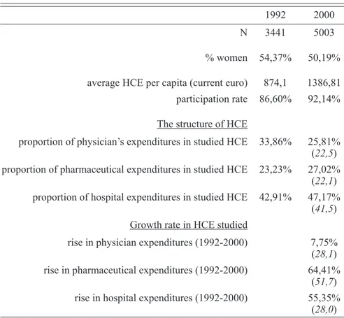
Table 1 presents the general characteristics of our sample. 3,441 individuals are observed in 1992 and 5,003 in 2000. The italics besides the percentages in the structure of health care expenditures studied refer to the corresponding proportions given for the whole population by the French Health Care Financing Administration. It can be seen that the overall proportion of each type of expenditure in our sample is relatively close to what is observed at the national level. Notice that we chose not to remove outliers from the data: indeed, removing the individuals who incurred the highest expenditures jeopardizes the representativity of each aggregate, par-ticularly hospital expenditures.

TABLE 1

Characteristics of the sample

1992 2000

N 3441 5003

% women 54,37% 50,19%

average HCE per capita (current euro) 874,1 1386,81

participation rate 86,60% 92,14%

The structure of HCE

proportion of physician’s expenditures in studied HCE 33,86% 25,81%

(22,5)

proportion of pharmaceutical expenditures in studied HCE 23,23% 27,02%

(22,1)

proportion of hospital expenditures in studied HCE 42,91% 47,17%

(41,5) Growth rate in HCE studied

rise in physician expenditures (1992-2000) 7,75%

(28,1)

rise in pharmaceutical expenditures (1992-2000) 64,41%

(51,7)

rise in hospital expenditures (1992-2000) 55,35%

(28,0) One feature of health data such as ours is that many individuals do not incur any expenditure. The level of expenditure is explained by the participation rate and by the conditional expenditure, conditional on participation. Figures 2a-i show for each type of expenditure (physician visits, medication and hospital expendi-tures) the age profi le of participation rate, conditional expenditure and uncondi-tional expenditure. The participation rates of physician visits and pharmaceutical expenditures are quite high (around 90%). The observed change in the participation

(9)

profi le has therefore a small impact on the unconditional expenditure. For these expenditures, the conditional and unconditional expenditures profi les are very similar (see fi gures 2e and 2f). This is not the same for hospital expenditures, for which the participation rate is quite low (between 10% and 20%): changes in the participation profi le have a greater impact on the fi nal profi le, which shows a size-able drift between 1992 and 2000 for people age 50 and over. These features show that ambulatory care and hospital care need separate analyses.

For physician and pharmaceutical expenditures, the profi le (conditional and unconditional on participation) is clearly increasing with age. A noticeable upward drift of this profi le appears for people age 40 and over between 1992 and 2000.

The drift is spectacular and signifi cant for pharmaceutical

expendi-tures, whereas it appears to be non signifi cant for physician

consulta-tions6_.

For hospital expenditures (conditional and unconditional), an upward drift is noticeable for people age 60 and over only (fi gure 2i). Participation rate for hospi-tal care has signifi cantly increased between 1992 and 2000, for all age groups. This rise in participation explains the shape of the unconditional expenditures profi les:

the corresponding drift is signifi cant ( , due to age groups 60 and 70 and

over) whereas the drift for conditional expenditures is not signifi cant .

The unconditional hospital expenditure fi gure might give support to the argu-ment of Zweifel et al. and Seshamani et al., namely that proximity to death is the main driver of hospital costs. Indeed, the expenditure profi le is relatively fl at until the 50-59 age group, then becomes very sloping (fi gure 2i). Yang et al. show that the age profi le of Medicare expenditures (which are mainly determined by hospital costs) is strongly infl uenced by the costs incurred by people who deceased within the year. Our data allowed us to compare, for year 2000, the expenditure age profi les of all individuals vs. individuals which were still alive in 2004 (“survivors”). We observe that the slope is less steep, but still sizeable for survivors: the shape of the hospital expenditures profi le is not only due to the dying (Dormont et al., 2006).

3 Morbidity and Age

We have paid attention to the building and testing of relevant morbidity indica-tors. Indeed, the level of morbidity by age group and its changes over time play a central role in our empirical evaluation. Our dataset gives us access to detailed information about every individual’s health status and the illnesses he/she might suffer from. In addition, information is recorded about the individual’s character-istics and habits, such as his/her size, his/her body mass index (BMI), whether he/she is a regular smoker and about socioeconomic variables such as employment

6. We have implemented tests to check for the signifi cance of the drifts observed in the profi les. Global signifi cance tests have been carried out, as well as separate tests for each age group. Results are provided below fi gures 2a-i: we give the age groups for which a signifi cant drift is observed and the p-value of the global signifi cance test.

(10)

status (employed-unemployed-retired) and whether or not he/she receives allow-ances from the public assistance. None of these variables is used as a regressor in our equations of participation and consumption. Therefore they can be used as instrumental variables to test for the exogeneity of morbidity indicators.

The information at our disposal results from answers of the individual to the sur-vey. Physicians check the survey and correct for discrepancies between objective information (e.g., type of medication taken) and declaration. Synthetic indicators have been built, such as the number of illnesses, the level of disability (8 levels) and the level of death risk. This latter variable is a grade given by the physicians who recode the survey, relative to the probability of death within the following fi ve years. It has six levels, from 0 (zero death risk) to 5 (surely negative prognosis). In addition, we have built indicators for chronic diseases, such as Hypertension, Diabetes, etc (altogether 10 illnesses). All potential indicators are detailed in appen-dix A. The process of selection and testing is described in appenappen-dix B, leading to the indicators fi nally selected.

3.1 Selecting Exogenous Morbidity Indicators

If health care is effective, health status is not an exogenous regressor for medi-cal expenditure. Logimedi-cally, its exogeneity depends on the delay between expendi-ture and potential health improvements. The fact that our database is composed of 2 cross-sections relative to yearly expenditures has consequences on the regres-sors’ exogeneity: chronic diseases are likely to be exogenous. Medical care cannot remove the cause but delay or prevent the consequences of these diseases. The most prevalent chronic diseases (diabetes, hypertension, or heart disease) cannot be cured and their onset is independent from the amount of medical care provided to the individual. On the other hand, procedures such as hip replacement improve substantially the patient’s state: disability may be endogenous.

Most analyses of the impact of ageing on expenditures have included health sta-tus as a control in the relationship, without any way of testing whether the variables used to measure health status were exogenous. Thanks to the richness of our data, which make many instrumental variables available, we were able to perform exo-geneity tests. For that purpose, we assumed that chronic diseases were exogenous. But the exogeneity of disability has been tested, as well as the exogeneity of syn-thetic indicators, such as death risk, self-assessed health and number of diseases. The procedure used is detailed in section 5.

3.2 Morbidity and Health Expenditures Profi le

It is well known that morbidity is increasing with age. This appears clearly in fi gures 3, which display the average level by age group of 4 morbidity indicators.

A simple OLS analysis performed on untransformed data shows that the fact that health expenditures are increasing with age is entirely due to the increase in morbidity with age. Figure 4 presents the contribution of each one of 3 sets of variables explaining the level of conditional pharmaceutical expenditures in a basic untransformed linear model: age dummies, morbidity indicators and socio-eco-nomic characteristics (gender, income, coverage, social and occupational group,

(11)

level of education)7_{. The fi gure shows clearly that age dummies do not infl uence} the expenditure profi le, once morbidity in taken into account.

7. This was obtained for the year 2000. Comparable graphs can be obtained for the year 1992 and other types of expenditures. The same kind of results has been obtained as regards participation rate: the increasing profi le of the use of health care services with age is mainly explained by the evolution of morbidity with age.

(3a) Disability

FIGURES 3

Changes in prevalence for four morbidity indicators

(3b) Death risk

(3c) Diabetes (3d) Arthritis, arthropathy and/or back pain

FIGURE 4

(12)

3.3 Changes in Morbidity Over Time

Figures 3 illustrate the changes in morbidity by age profi les that occurred between 1992 and 2000. These graphs are representative of what is found for our various indicators. For most of them, there is a decrease in the level of morbidity over time, i.e. a health improvement. However, this is not systematic and not homogenous among age groups. For instance, the frequency of diabetes is decreasing for all age groups between 1992 and 2000, but increases for individuals aged 70 and over (fi gure 3c). On the other hand, the frequency of arthritis and back pain is increasing for each age group (fi gure 3d).

These results do not allow to draw any general conclusion about a health improve-ment hypothesis: the prevalence is increasing or decreasing, depending on the mor-bidity indicator and the age group considered. Our estimation approach allows us to evaluate the resulting effect of all these changes on expenditure by age group. In other words, it is possible to synthesize the total impact of changes in morbidity. Anticipating on our results, we fi nd that this impact is negative, indicating that the health status of individuals is improving, indeed.

4 The Empirical Approach

The purpose of our simulations is to examine the infl uence of various effects on the shifts in the age-profi le of health expenditures. Our empirical approach entails three steps: fi rstly, the specifi cation and estimation of a two-equations model explaining the decision to consume and the level of expenditure, conditional on participation; secondly, the use of the estimates to simulate counterfactual aver-age levels of participation and expenditure by aver-age group. This second step makes it possible to assess the impacts of changes in morbidity and changes in practices between 1992 and 2000. In the third step, we use the microsimulation results to evaluate, at the macroeconomic level, the respective effects of demographic changes (ageing) and profi le drifts (changes in morbidity and practices) on health expenditure growth.

This approach is implemented for each of the three components of health care expenditure we focus on: physician consultations, pharmaceutical consumption, hospital expenditures.

4.1 Econometric Specifi cations and Estimation

A typical feature of health expenditure data is that many individuals incur no health costs within the period of observation. The descriptive analysis has shown the high proportion of non-users for hospital. As regards consultations and drugs, the proportion of non-users, although smaller, is not negligible. Such a confi gura-tion requires specifi c estimagura-tion techniques. Many papers addressed the issue of the choice between the sample-selection model (Heckman, 1979) and the two-part

(13)

model (Dow et al., 2002; Leung et al., 1996; Manning et al., 1987). Monte Carlo studies implemented by Manning, Duan and Rogers show that the two-part model performs better than the sample selection model even when the latter is the true model. Leung and Yu have shown that the performances of the sample selection model depend crucially on the degree of collinearity between the inverse Mill’s ratio and the explanatory variables in the second step equation. When there is no collinearity, a t-test of the coeffi cient of the inverse Mill’s ratio can be used to choose between the two specifi cations. On the other hand, collinearity problems make the two-part model more reliable because it performs better in terms of mean-squared error than the sample-selection model.

Our data is characterized by a high correlation between the inverse Mill’s ratio and the explanatory variables of the second step equation: the correlation coeffi cient lies between 0.85 and 0.87, depending on the health expenditure component consid-ered. Therefore, we chose the two-part model, which presents another advantage: it permits the use of a generalized linear model (GLM) to estimate the level of con-sumption, conditional on participation. The GLM makes it possible to deal rather easily with other typical features of health consumption data, such as skewness in the raw-scale variable, heavy-tailed distributions and heteroscedastic errors. Indeed,

the GLM approach makes it possible (i) to avoid the retransformation diffi culties8_by

specifying directly the expectancy of expenditure instead of the Log of expenditure, to allow for heavy-tailed distributions and heteroscedastic errors by considering Poisson or Gamma distributions for the dependent variable (Manning et al., 2001).

Consider individual i belonging to age group j. We denote the dichotomic

variable for participation and the health care consumption and consider the

following model: (1)

where .

(2)

We decided to use for (2) a log link relationship: is defi ned as an

exponential function of . Indeed, the non-zero observations for health

expen-ditures are highly skewed (the skewness varies between 4.50 and 15.47, depending on the year and type of expenditure considered). Taking the log transformation reduces the skewness to values between -0.26 to 0.01. In addition, we used for a gamma distribution, which enables us to take heteroskedasticity into account.

8. In the case of a loglinear specifi cation, where log( )y = β +x u, predicting y on the untransformed scale is not so easy because E y x( )= E_exp(xβ +u x) _. This latter expression is proportional to exp( )xβ

(14)

The choice of a gamma distribution is based on the outcomes of Park tests that we have performed, following the approach suggested by Manning and Mullah.

Equation (1) describes the decision to use health care services and equation (2) the level of consumption.

and are the explanatory variables of the participation and

consump-tion equaconsump-tions. These regressors entail dummies a_j and related to the age groups

and morbidity indicators . In addition, equations (1) and (2) include

explana-tory variables (variables or ) relative to socio-economic characteristics of

the individual. The potential list of morbidity indicators include disability, death risk, the number of illnesses, self-assessed health, and indicators for the follow-ing illnesses: diabetes, chronic obstructive pulmonary disease and related dis-eases, ischemic heart disease, hypertension, circulatory disease, conditions associ-ated with lipid metabolism, depression, sleeping disorder, cataract, and arthritis, arthropathy and/or back pain. The potential list of socio-economic characteristics include level of earnings, social and occupational group, education level, coverage by a complementary insurance, gender, family size and matrimonial status. The effective list depends on the equation ((1) or (2)) and on the type of expenditure considered (physicians, pharmaceutical or hospital): it has been set by a careful selection process described in appendix B.

As stated in section 3, some morbidity indicators may be non exogenous. Chronic diseases are likely to be exogenous. On the other hand, disability and synthetic indicators of health status, such as death risk, self-assessed health and number of diseases may be non exogenous. In addition, the coverage by a complementary insurance may be non exogenous, since it results partly from an individual deci-sion. We have chosen to select only exogenous regressors to avoid adding method-ological diffi culties to an already rather sophisticated approach.

Thanks to the richness of our data, we were able to perform Hausman tests for consultations, pharmaceutical and hospital expenditures. This was possible for year 2000 only. Not enough instruments were available for 1992, where the survey did not record enough information about socioeconomic variables nor about individual characteristics and habits. Nevertheless, it seems to us legitimate to assume that exogeneity checked for 2000 holds for 1992.

We used intrumental variables to build a Hausman specifi cation test for each of the three types of health care consumption, following Rivers and Vuong’s (1988) approach for the participation equation and using a log-linear model for the consump-tion equaconsump-tion. A Sargan test was used to check the validity of the instruments used. In addition, we examined whether this test could be subject to the weak instrument problem (Staiger and Stock, 1997). For this purpose, we tested for global signifi cance of the instruments in a system equation model (Seemingly Unrelated Regressions [SUR]) comprising several equations, where each instrumented variable is explained by the instruments and the exogenous regressors. Detailed list of intruments used and outcomes of the tests are provided in appendix B. We found a large signifi cance of the partial correlation between instruments and morbidity indicators, with high statistics

and levels of signifi cance lower than 10–3_{. Sargan tests validated the exogeneity of}

the instruments. Coverage by a complementary insurance appear to be exogenous for consultations and pharmaceutical expenditures (it is not a signifi cant regressor for hospital). Exogeneity is rejected for disability as regards consultations expenditures and for death risk as regards pharmaceutical expenditures.

(15)

4.2 Predictions and Simulations

For individual i of age group j, the decision to use health care services is easily predicted from the estimation of (1) by a Probit estimator:

(3)

with standing for the cdf of the standard normal distribution.

As concerns conditional expenditures, the GLM specifi cation leads to a direct estimate of the conditional expectancy of expenditures on the raw scale:

(4)

The model is estimated separately for years 1992 and 2000 for each type of expenditures (consultations, pharmaceutical, hospital), leading to estimated

coef-fi cients , , and .

Since the computation of predictors (3) and (4) involve several non-linear func-tions, we cannot exhibit additive effects. We use instead an incremental approach. As concerns the decision to use health care services (participation), we compute or simulate the predicted probability for the average patient of each age group j. This is done for each expenditure component, i.e. physician visits, drugs and hospital.

For the population observed in 1992, the predicted probability of using health care services is the following:

This probability is evaluated at the average point of each age group: (5)

We have chosen this approach instead of computing the average by age group of individual predicted probabilities. Indeed, counterfactual simulations on popula-tion characteristics are possible at the age group level only.

The effect on participation of changes in practices for a given morbidity is

assessed by replacing by in expression (5):

(16)

The incremental effect of changes in morbidity between 1992 and 2000 is assessed by replacing, for each age group, the average level of morbidity observed

in 1992, by the average level of morbidity observed in 2000, :

(7)

Finally, the incremental effects of other changes in behavior and individual char-acteristics lead to the predicted probability for the year 2000:

(8)

We used expression (4) to compute similarly the predictions of the levels of

expenditures by age group, conditional on participation: , ,

and . More precisely, the means by age group of the

explanatory variables are computed on the subsamples of participants, when simu-lating the conditional expenditures. We have the following transitions:

The transition from to gives the effect of changes in

practices for a given morbidity.

The transition from to gives the incremental effect

of changes in morbidity (among the participants) between 1992 and 2000.

Finally, the transition from to gives the incremental

effect of other changes of behavior and individual characteristics between 1992 and 2000.

At each step, unconditional expenditure C is computed as the product .

Broadly understood, changes in practices are changes in the estimated param-eters of (1) or (2) between 1992 and 2000. These changes are linked to changes in patients’ or physicians’ behavior. They also result from technological prog-ress, which induces the use of more costly innovative drugs and procedures. As explained in section 2.1, this technological progress may concern the extension of innovative procedures and prevention protocols to old ages.

We capture changes in practices for a given morbidity with changes in the estimated vectors and . These estimated coeffi cients measure the infl uence of morbidity on participation rate and expenditures. What we call “other changes in behavior and individual characteristics between 1992 and 2000” can also be interpreted as changes in practices. Actually, these “other changes” depend on changes in the variables W

and Z, as well as changes in the parameters , , and . To make the graphs

relative to the micro simulations readable, we did not present separately the effects of changes in the age-specifi c constants. But this is done in the recapitulative table of

●

(17)

section 6, where we make the evaluations at the macroeconomic level. These changes in age-specifi c constants can be linked to changes in unobservable morbidity as well as changes in practices for a given level of morbidity.

Our microsimulation method is in the spirit of the Oaxaca (Oaxaca, 1973) meth-odology. It has been recently used to analyse the process of technological progress diffusion within French hospitals (Dormont et al., 2006).

5 Microeconometric Results

5.1 Estimations

As was mentioned in section 4, the variables explaining participation and condi-tional expenditure were carefully selected. Only those that proved to be signifi cant and exogenous were kept for the estimations and simulations.

The estimation of equations (1) and (2) reveals a strong infl uence of morbidity on

participation and conditional consumption9_{. The morbidity indicators, the number}

of diseases and the levels of disability and death risk have large positive impacts

on the use of health care services. To take an example, in 1992, a disability level10

equal to 3 incurs an increase in conditional pharmaceutical consumption of 42 %.

When the disability level11_{is equal to 4 or 5, the rise in the conditional}

pharma-ceutical consumption amounts to 77% and 89%. The conditional pharmapharma-ceutical consumption is also strongly infl uenced by hypertension (+40%), diabetes (+ 48%)

trouble with lipid metabolism (+ 25%) and depression (+ 37%)12_{. Participations}

to consultation and pharmaceutical consumption are also signifi cantly infl uenced by our morbidity indicators. The conditional consultation expenditure is positively infl uenced by depression (+27 %) and the number of diseases. Turning to hospital expenditure, participation appears to be positively infl uenced by diabetes, death risk and cataract, and the level of conditional expenditure by the level of disability and hypertension (+37%).

Otherwise, we fi nd that the absence of privately subscribed complementary cov-erage signifi cantly reduces participation and consumption of ambulatory care. For example, in 1992, the drop amounts to -39% for conditional physician expendi-tures and to -25% for conditional pharmaceutical expendiexpendi-tures. On the other hand, complementary coverage has no signifi cant infl uence on the use of hospital care. In general, gender is not signifi cant for participation, but being a female increases consultation and pharmaceutical expenditures by about 17%. Gender is not signifi -cant for hospital expenditures.

9. We do not display the detailed results here. They are available on request.

10. Disability level 3 corresponds to a situation where the individual “experiences diffi culties but lives normally”.

11. Disability level 4 corresponds to a situation where the individual “must diminish his/her domestic or professional activity”. Level 5 encompasses situations as “diminished activity”, “no domestic autonomy” and “confi ned to bed”.

(18)

Most of the positive coeffi cients estimated for the morbidity indicators in 1992 are larger in 2000. It clearly shows that changes in practices result in more expen-ditures in 2000 than in 1992, for a given morbidity.

5.2 Simulations

The simulations we implemented led to the calculation of average probabilities of participation and conditional expenditures for each age group j, at each step of

the reasoning. Namely, the values , , and were

com-puted for participation and , , and

for the conditional expenditures. At each step of simulation, unconditional

expen-diture C is computed as the product . The resulting profi les by age group

are displayed in fi gures 5a-i. For each variable of interest, the drift between the pro-fi le of 1992 (propro-fi le 1) and the propro-fi le of 2000 (propro-fi le 4) is split into 3 incremental

effects: the transition from profi le 1 to profi le 2 gives the effect of changes in

practices for a given observable level of morbidity; the transition from profi le

2 to profi le 3 gives the effect of changes in morbidity; the transition from

profi le 3 to profi le 4 gives the effect of other changes in behavior and individual characteristics. Ambulatory care (physician and pharmaceutical expenditures) and hospital expenditures show fairly different results, which are worth treating sepa-rately.

FIGURE 5F (ZOOMED)

(19)

FIGURE 5I (ZOOMED):

Simulated unconditional hospital expenditures

Profi le 1: predicted expenditure, 1992. Profi le 2: expenditure with population characteristics of 1992 and morbidity coeffi cients of 2000 (counterfactual simulation). Profi le 3: expenditure with population characteristics of 1992, morbidity coeffi cients of 2000 and morbidity level of 2000 (counterfactual simulation). Profi le 4: predicted expenditure, 2000.

Transition 1 to 2: drift due to changes in practices for a given morbidity level. Transition 2 to 3: incre-mental drift due to changes in morbidity. Transition 3 to 4: increincre-mental drift due to other changes.

5.2.1 Ambulatory Care

For ambulatory care, the bulk of changes is essentially due to changes in expen-ditures conditional on participation and not to changes in participation. Changes in participation rate have a very small infl uence on unconditional expenditures pro-fi le drifts. Indeed, participation to ambulatory care is already very high in 1992 (between 80% and 98%): changes that occurred in 2000 are necessarily limited.

The drift in the age profi le of expenditures is much more spectacular for phar-maceutical expenditures than for physician consultations, whose drift is globally

non signifi cant13_{. This appears when comparing fi gures 5c and 5f, keeping in mind}

that scales differ.

As concerns physician expenditures, one observes a small negative drift due to changes in practices (fi gure 5c, profi le 1 to 2): for a given illness, less consulta-tions are used in 2000 than in 1992. A positive drift, which is mainly due to “other changes” offsets this negative impact: on the whole, changes between 1992 and 2000 are not signifi cant as regards physician expenditures.

Drugs are responsible for the bulk of the growth in total health care expendi-tures. The pharmaceutical expenditures rise tremendously: the changes are clearly observable in the zoomed fi gure 5f. Our simulations show that this growth is almost entirely due to a large upward drift in relation to changes in practices for a given observable level of morbidity (profi le 1 to 2). The changes in morbidity induce a downward drift which compensates only partly this upward drift. Our results sug-gest that there is a large innovation component: the drift is not due to changes in

(20)

(5a) (5b) (5c) (5d) (5e) (5f)

(21)

(5g) (5h) (5i) F IGURES 5 Pro fi le 1: predicted expenditure, 1992. Pro fi

le 2: expenditure with population characteristics of 1992 and morbidity coef

fi

cients of 2000 (counterfactual simulation).

Pro

fi

le 3: expenditure with population characteristics of 1992, morbidity coef

fi

cients of 2000 and morbidity level of 2000 (counterfactual

simulation). Pro

fi

le 4: predicted expenditure, 2000.

T

ransition from pro

fi

le 1 to pro

fi

le 2: drift due to changes in practices for a given morbidity level. T

fi

le 2 to pro

fi le

3:

incremental drift due to changes in morbidity

. T

fi

le 3 to pro

fi

(22)

the behaviour of the elderly, but is rather linked to the supply of new products on the health care market.

5.2.2 Hospital

What is observed for hospital care contrasts strongly with ambulatory care, in the sense that changes are mainly due to a drift in the participation profi le by age (see fi gure 5g). The drift in participation rates is observed for every age group and is increasing with age. Our simulation shows that this upward drift is due fi rstly to the “other changes” and secondly to changes in practices for a given level of morbidity. The upward drift due to the changes in practices (profi le 1 to 2) is noticeable for the more than 50 year-olds, along with a slight downward drift due to the changes in morbidity for these same age groups.

As for hospital unconditional expenditures, we fi nd again the negative effect of changes in morbidity for people age 40 and over, as well as the positive effect of changes in practices for a given morbidity. One observes for the two last age groups a tremendous drift due to the combined effects of changes in practices and “other changes”. This jump is only visible on fi gure 5i (unconditional expenditures), since it stems from the changes in participation behaviour.

6 Accounting for the Effects

of Ageing and Changes in Practices

at the Macro Level

On table 2, we applied the predictions and simulations derived above to the French population. This allows us to evaluate retrospectively the relative effects of the demographic change and profi le drifts that occurred between 1992 and 2000. In addition, we can evaluate the components of changes in profi le drifts.

The total demographic effect is computed assuming that the 1992 age profi le of expenditures is held constant, and that only the structure and size of the population changed over time. The other effects are then computed by using the different sim-ulated profi les. A bootstrap analysis has been performed to assess the signifi cancy of these results (bootstrap by pairs, 800 replications).

We fi nd again the negative effect of changes in morbidity. The rise in health care expenditures due to the demographic change appears to be very small, in compari-son with the effects of changes in practices. For total expenditures, we fi nd that the impact of changes in practices is equal to +12.9%. Thus, it is 3.8 times larger than the rise in health care expenditures due to changes in the age structure of the population (+3.4%). Moreover, we fi nd that the impact of changes in morbidity is negative, indicating an improvement of the health status of individuals for a given age. This is true for total expenditure but also for each type of expenditure. For total expenditure, this negative effect of changes in morbidity (-9.7 %) more than com-pensates the positive shock due to changes in the age structure of the population (+3.4 %). This is also true for pharmaceutical and hospital expenditures. Drawing a rapid conclusion, one could ask whether the population is ageing at all.

(23)

TABLE 2

Simulations at the macro level

Variation 1992-2000 (%) Physicians Pharmac. Hospital Total

Total demographic change 5,05 7,63 6,37 6,35

of which:

part of structural change 2,10 4,61 3,38 3,36

part of growing size

of population 2,95 3,02 2,99 2,99

Changes in practices for a

given morbidity -15,09 52,24 7,06 12,87

Changes in morbidity -1,23 -9,24 -14,61 -9,74

Changes in age dummies 28,63 14,11 -26,25 -1,55

Other changes -2,80 2,53 95,51 45,95

Total variation 1992-2000 (%) 14,57 67,27 68,08 53,89

7 Conclusion

Our results show that ageing is likely to explain only partially the rise in health care expenditures. The main explanation of expenditure growth is linked to changes in practices. For ambulatory care, changes in practices for the elderly are not linked to changes in participation behaviour but to changes in conditional consumption. The drift due to changes in practices is spectacular for pharmaceutical expenditures, sug-gesting a large innovation component. These results reveal that the drifts we observe are not due to changes in the behaviour of the elderly. They are connected rather to the supply side, that is, to the introduction of new products on the health care market. Our study is not restricted to hospital expenditures. Indeed, our data allow us to split health care expenditures into three components: physician, pharmaceutical and hos-pital expenditures. Because we were able to consider pharmaceutical expenditures separately, we were able to show that the upward drift in drug consumption is mainly due to the supply of new products, i.e. to technological progress. Taking participation into account in our model allowed us to isolate changes that might be due to patients’ initiative. Our results suggest that they are of little importance.

Another advantage of our database is that it provides information about

mor-bidity indicators. This enabled us: to show that the health of the elderly is

improving to evaluate the savings due to changes in morbidity. Health care

expenditures are too often conceived of as a burden and it is indeed very diffi cult to measure their benefi t in terms of health improvement. Our fi ndings give evidence of health improvements.

We have shown that changes in practices appear to be the main driver in the increase in expenditures. It is possible that technological progress is oriented towards the elderly more than other age groups. In that case, the impact of changes

(24)

in practices would increase with age. Due to our data limitations, we were not able to estimate slopes specifi c to each age group in order to study this question. Further investigation with larger samples will allow us to study the pattern of technological progress diffusion more thoroughly.

References

BAC C. and CORNILLEAU G. (2002). – « Comparaison internationale des dépenses de santé : une

analyse des évolutions dans sept pays depuis 1970. » Etudes et Résultats, DREES, 175. BAUBEAU D., BOUSQUET F. and JOUBERT M. (2001). – « Le traitement chirurgical de la

cata-racte en France », Etudes et Résultats, DREES, 101, 2001.

DORMONT B., GRIGNON M. and HUBER H. (2006). – “Health Expenditure Growth: Reassessing

the Threat of Aging”, Health Economics, 15: pp. 947-963.

DORMONT B., and MILCENT C. (2006) « Innovation Diffusion under Budget Constraints.,

Annales d’Economie et de Statistique, n° 79/80.

DOW W.H. and NORTON E.C. – “The Red Herring that Eats Cake: Heckit Versus Two-Part Model

Redux”, February 2002. Triangle Health Economics Working Paper Series - www.unc.edu/the. GERDTHAM U.G., JONSSON B., MACFARLAN M. and OXLEY H. (1998). — Health, the Medical

Profession and Regulation, chapter “The Determinants of Health Expenditure in the OECD Countries: a Pooled Data Analysis”, pages 113-134. Kluwer Academic Publisher. GERDTHAM U.G., SOGAARD J., ANDERSSON F. and JONSSON B. (1992). – “An Econometric

Analysis of Health Care Expenditure: a Cross-Section Study of the OECD Countries”, Journal of Health Economics, 11, pp. 63-84.

GETZEN T.E. (1992). – “Population Aging and the Growth of Health Care Expenditures”,

Journal of Gerontology, 47: pp. S98-S104.

HECKMAN J.J. (1979). – “Sample Selection Bias as a Specifi cation Error”, Econometrica,

47:153-161.

HITIRIS T. and POSNETT J. (1992). – “The Determinants and Effects of Health Expenditure in

Developed Countries”, Journal of Health Economics, 11:173-181. IRDES Institute Paris France. Eco-Santé 2002 Database.

LEU R.E. (1986). — Public and Private Health Services: Complementarities and Confl icts,

Chapter “The Public-Private Mix and International Health Care Costs”, pp. 41-63. Blackwell Scientifi c Publications.

LEUNG S.F. and YU S. (1996). – “On the Choice Between Sample Selection and Two-Part

Models”, Journal of Econometrics, 72: pp. 197-229.

MANNING W., DUAN N. and ROGERS W. (1987). – “Monte Carlo Evidence on the Choice Between

Sample Selection and Two-Part Models”, Journal of Econometrics, 35: pp. 59-82.

MANNING W.G. and MULLAHY J. (2001). – “Estimating Log Models: to Transform or not to

Transform?”, Journal of Health Economics, 20: pp. 461-494.

OAXACA R. (1973 ) “Male-Female Wage Differentials in Urban Labor Markets”, International

Economic Review, 14 : pp. 693-709

O’CONNELL J. (1996). – “The Relationship Between Health Expenditures and the Age

Structure of the Population in OECD Countries”, Health Economics, 5: pp. 573-578. OBERLIN Ph., MOUQUET M.-C. and FOLLIGUET Th. (february 2004). – « Le traitement invasif

des maladies coronariennes », Etudes et Résultats, DREES, 289.

OECD (1987). – Financing and Delivering Health Care: a Comparative Analysis of OECD Countries.

RIVERS D. and VUONG Q. (1988). – “Limited Information Estimation and Exogeneity Tests

for Simultaneous Probit Models”, Journal of Econometrics, 39: pp. 347-366.

SANDIER S., POLTON D., Paris V. and Thomson S. (2002). – Health Care Systems in Eight

Countries: Trends and Challenges, chapter “France”, pp. 31-45. The European Observatory on Health Care Systems.

SESHAMANI M. and GRAY A.M. (2004a). – “A Longitudinal Study of the Effects of Age and

(25)

SESHAMANI M. and GRAY A.M. (2004b). – “Aging and Health-Care Expenditure: the Red

Herring Argument Revisited”, Health Economics, 13: pp. 303-314.

STAIGER D. and STOCK J.H (1997). – “Instrumental Variables Regression with Weak

Instruments”, Econometrica, 65: pp. 557-586.

STEARNS S.C. and NORTON E.C. (2004). – “Time to Include Time to Death? the Future of

Health Care Expenditure Predictions”, Health Economics, 13: pp. 315-327.

YANG Z., NORTON E.C. and STEARNS S.C (2003). – “The Real Reasons Older People Spend

More”, Journal of Gerontology: Social Sciences, 58B(1): pp. S1-S10.

ZWEIFEL P., FELDER S. and Meiers M. (1999). – “Ageing of the Population and Health Care

(26)

Appendices

A Variables Potentially used in the Estimations

A.1 Short Summary of the Variables

Age group Gender

Marital status (abbreviated mstatus) Size of household (abbreviated hhsize) Level of education

Social and occupational group of the head of household (following the usual

French Standard Occupational Classifi cation, abbreviated SOC)

Household net income per consumption unit (abbreviated Income) Absence of supplementary coverage (abbreviated Supplcov) The indicators of morbidity described below

A.2 The Age Groups

0: 0-9 years old 10: 10-19 years old 20: 20-29 years old 30: 30-39 years old 40: 40-49 years old 50: 50-59 years old 60: 60-69 years old 70: 70 years old and older

A.3 Socio-Demographic Characteristics

Marital status

1: married or living in a couple 2: divorced or separate 3: widow / widower 4: single

Level of education

1: does not go to school, never went to school, other 2: kindergarten to primary school

3: junior high school 4: high school 5: higher education

Social and occupational group (INSEE classifi cation)

1: farmers 2: independent workers 3: intellectual professions 4: intermediary professions ● ● ● ● ● ● ● ● ● ● ● ● ● ● ● ● ● ● ● ● ● ● ● ● ● ● ● ● ● ●

(27)

5: clerks

6: qualifi ed workers 7: non-qualifi ed workers

Household net income per consumption unit

1: belonging to the 20% lowest incomes

2: belonging to the middle 40% of the income distribution 3: belonging to the 20% highest incomes

A.4 The Indicators of Morbidity

They are eventually to be tested for adequacy in the econometric model: signifi -cancy is tested for all and exogeneity is tested for the synthetic morbidity indicators.

A.4.1 The Synthetic Morbidity Indicators:

The level of disability: (levels 5 to 7 are grouped together)

0: no diffi culty

1: very small level of diffi culty 2: small level of diffi culty

3: experiences diffi culties but lives normally

4: must diminish his/her domestic or professional activity 5: diminished activity

6: no domestic autonomy 7: confi ned to bed

The death risk (DR):

0: level zero of death risk 1: very low negative prognosis 2: low negative prognosis 3: possible risk

4: probably negative prognosis 5: surely negative prognosis

The level of death risk (probability of death within the following 5 years) is elaborated by the IRDES physicians who recode the survey.

The number of illnesses (nbpath) is calculated from the list of illnesses declared

by the respondent, coupled with the ones found out by the physicians recoding the survey, on the basis of other elements of the survey, such as the type of medication taken.

The self-assessed health (SAH) is captured through a grade declared by the

survey individual who rates his/her health from 0 (poorest) to 10 (highest).

A.4.2 The Chronic Illnesses

The chosen chronic illnesses specifi cally affect the elderly. They were selected following the ICD-10 with the help of C. Sermet (M.D.) from the Irdes Institute. As the ICD (International Statistical Classifi cation of Diseases and Related Health Problems) has changed between 1992 and 2000 from ICD-9 to ICD-10, we had for the purpose of our study to use a correspondence between the two classifi cations elaborated by the IRDES institute. It consists in corresponding broad groups of

● ● ● ● ● ● ● ● ● ● ● ● ● ● ● ● ● ● ● ●

(28)

diseases; the corresponding morbidity dummy variable codes the fact of suffering from at least one disease from the group. The such groups eventually chosen are the following:

diabetes

chronic obstructive pulmonary disease and related diseases (abbreviated

COPD)

ischemic heart disease (abbreviated Heart) hypertension

circulatory disease

conditions associated with lipid metabolism (abbreviated Lipid) depression

sleeping disorder cataract

arthritis, arthropathy and/or back pain (abbreviated arthrodorso).

B The Selection of Variables

For each kind of expenditure (physician, pharmaceutical and hospital expendi-ture) and each step of estimation (participation and conditional expendiexpendi-ture), an estimation was led with all the potential variables in order to select the signifi cant ones. The results below provide the list of the selected variables along with the ones that were eliminated, with the result of a global signifi cance test of the latter.

For each step of analysis (participation and conditional expenditure), the exo-geneity analysis uses the selected signifi cant variables along with supplementary instruments described below (which may vary according to the equation stud-ied).

For the fi nal estimations and simulations, only the signifi cant and exogenous vari-ables were kept. This appendix recapitulates this choice process for each expendi-ture studied: signifi cance analysis and exogeneity tests. Also provided are for each

kind of expenditures the R2_{of the regression of the estimated inverse Mill’s ratio}

on the selected second step variables, that indicates the degree of correlation of the two used to assess the validity of the GLM.

B.1 Physician Expenditures

B.1.1 Signifi cance Analysis

Participation (probit)

Selected: age, income, SOC, hhsize, education, mstatus, hypertension, lipid, nbpath, supplcov

Eliminated: gender, COPD, heart, circulatory disease, depression, sleeping disor-der, cataract, arthrodorso, DR, disability, SAH, diabetes

● ● ● ● ● ● ● ● ● ●

(29)

Test for H_o: the eliminated variables are not signifi cant: chi2(12)=15.14, p=0.2339

Conditional expenditure

Selected: age, gender, SOC, education, depression, disability, nbpath, SAH, sup-plcov

Eliminated: income, diabetes, COPD, heart, hypertension, circulatory disease, lipid, sleeping disorder, cataract, arthrodorso, DR, hhsize, mstatus

Test for H_o: chi2(16)=20.12, p=0.2148

R2_{of the} _{regressed on the second step variables:} _(the

correla-tion coeffi cient between the two is thus

B.1.2 Exogeneity Test of the Synthetic Morbidity Indicators and Suppl. Coverage

Instruments: head of household status (working, unemployed, non-working, the reference being retired), smoking, receiving minimum benefi t payment

Sargan test (validity of instruments): chi2(3)=3.150, p=0.3691 Weak instruments: chi2(10)=415.05, p=0.0000

Tested variables: nbpath, supplcov Exogenous variables: nbpath, supplcov Rivers & Vuong test: chi2(2)=1.26, p=0.5336 Conditional expenditure

Instruments: head of household status (working, unemployed, non-working, the reference being retired), smoking, receiving minimum benefi t payment, height, BMI (regular, overweight, obesity, the reference being underweight)

Tested variables: disability, nbpath, SAH, supplcov Exogenous variables: nbpath, SAH, supplcov Hausman test: chi2(5)=7.29, p=0.1996

B.2 Pharmaceutical Expenditures

Selected: age, gender, SOC, hhsize, education, mstatus, diabetes, hypertension, lipid, arthrodorso, nbpath, SAH, supplcov

(30)

Eliminated: income, COPD, heart, circulatory disease, depression, sleeping dis-order, cataract,DR, disability

Test for H_o: chi2(10)=5.25, p=0.8738

Selected: age, gender, hhsize, education, diabetes, hypertension, lipid, depres-sion, arthrodorso, DR, disability, nbpath, SAH

Eliminated: income, SOC, supplcov, COPD, heart, circulatory disease, sleeping disorder, cataract, mstatus

Test for H_o: chi2(17)=13.19, p=0.7233

correla-tion coeffi cient between the two is thus )

Instruments: head of household status (working, unemployed, non-working, the reference being retired), smoking, receiving minimum benefi t payment

Tested variables: nbpath, SAH, supplcov Exogenous variables: nbpath, SAH, supplcov Rivers & Vuong test: chi2(3)=1.56, p=0.6687 Conditional expenditure

Tested variables: DR, disability, nbpath, SAH Exogenous variables: disability, nbpath, SAH Hausman test: chi2(5)=9.47, p=0.0917

B.3 Hospital Expenditures

Selected: age, gender, hhsize, education, mstatus, diabetes, lipid, cataract, arthro-dorso, DR, disability, nbpath, SAH

(31)

Eliminated: income, SOC, supplcov, COPD, heart, hypertension, circulatory dis-ease, depression, sleeping disorder

Test for H_o: chi2(15)=15.57, p=0.4115

Selected: age, education, hypertension, arthrodorso, disability, nbpath

Eliminated: gender, income, supplcov, diabetes, COPD, heart, circulatory dis-ease, lipid, sleeping disorder, cataract, DR, SAH, hhsize, mstatus, SOC, depres-sion

Test for H_o: chi2(24)=32.57, p=0.1135

correla-tion coeffi cient be tween the two is thus )

Tested variables: DR, disability, nbpath, SAH Exogenous variables: DR, disability, nbpath, SAH Rivers & Vuong test: chi2(4)=3.20, p=0.5249 Conditional expenditure

Instruments: head of household status (working, unemployed, non-working, the reference being retired)smoking, receiving minimum benefi t payment, height, BMI (regular, overweight, obesity, the reference being underweight)

Tested variables: disability, nbpath Exogenous variables: disability, nbpath Hausman test: chi2(2)=0.19, p=0.9115

(32)