Rareté de l’eau et relations interbassins en Méditerranée sous changements globaux. Développement et application d’un modèle hydroéconomique à large échelle

(1)

HAL Id: tel-02925151

https://pastel.archives-ouvertes.fr/tel-02925151

Submitted on 28 Aug 2020

HAL is a multi-disciplinary open access archive for the deposit and dissemination of sci-entific research documents, whether they are pub-lished or not. The documents may come from teaching and research institutions in France or abroad, or from public or private research centers.

L’archive ouverte pluridisciplinaire HAL, est destinée au dépôt et à la diffusion de documents scientifiques de niveau recherche, publiés ou non, émanant des établissements d’enseignement et de recherche français ou étrangers, des laboratoires publics ou privés.

Noemie Neverre. Rareté de l’eau et relations interbassins en Méditerranée sous changements globaux. Développement et application d’un modèle hydroéconomique à large échelle. Economies et finances. Université Paris Saclay (COmUE), 2015. Français. �NNT : 2015SACLA002�. �tel-02925151�

(2)

NNT : 2015SACLA002

T

HÈSE DE DOCTORAT

DE

L’U

NIVERSITÉ

P

ARIS

-S

ACLAY

PRÉPARÉE AU

C

ENTRE

I

NTERNATIONAL DE

R

ECHERCHE SUR

L

’E

NVIRONNEMENT ET LE

D

ÉVELOPPEMENT

E

COLE

D

OCTORALE N

°

581 ABIES - Agriculture, alimentation, biologie, environnement et santé

Spécialité de doctorat : Sciences Économiques

Par

Noémie Neverre

Rareté de l’eau et relations interbassins en Méditerranée sous changements globaux

Développement et application d’un modèle hydroéconomique à large échelle

Thèse présentée et soutenue à Nogent sur Marne, le 17 septembre 2015 :

Composition du Jury :

M. Dumas, Patrice M. Hourcade, Jean-Charles M. Massarutto, Antonio M. Maugis, Pascal M. Polcher, Jan

M. Pulido Velázquez, Manuel M. Ward, Philip

Chercheur CIRAD

Directeur de recherche CNRS, Directeur d’études HESS Professeur, University of Udine, Italie

Chercheur, LSCE

Directeur de recherche CNRS

Professeur, Université Polytechnique de Valence, Espagne Chercheur, VU University Amsterdam, Pays-Bas

Directeur de thèse Directeur de thèse Rapporteur Examinateur Président Rapporteur Examinateur

(3)

Université Paris-Saclay

Espace Technologique / Immeuble Discovery

(4)

Water scarcity and inter-basin interactions

under global changes

A large-scale hydroeconomic model applied to the

Mediterranean region

Rareté de l’eau et relations interbassins en

Méditerranée sous changements globaux

Développement et application d’un modèle

hydroéconomique à large échelle

(5)

Noémie Neverre neverre@centre-cired.fr

Centre International de Recherche sur l’Environnement et le Développement

Campus du Jardin Tropical 45 bis, avenue de la Belle Gabrielle

(6)

Summary

Global socioeconomic and climatic changes will increase the pressure on wa-ter resources in the Mediwa-terranean region in the next decades. This thesis contemplates the question of how heterogeneously distributed water con-straints might foster inter-basin interactions. To do so, it is necessary to as-sess localised water scarcity in terms of both water quantities and economic values, in a framework combining a river basin level modelling with an ex-tended geographic coverage. The methodological approach used is generic hydroeconomic modelling.

The first part of the thesis is dedicated to the projection and valuation of water demands. For the domestic sector, the approach is to build three-part inverse demand functions, calibrated at the country scale, taking into account structural change. For the agricultural sector, the economic bene-fits of irrigation water are calculated based on a yield comparison approach between rainfed and irrigated crops.

The second part concentrates on the supply-side of the hydroeconomic model. Operating rules of the reservoirs and water allocation between de-mands are determined based on the maximisation of water benefits over time and space. A parameterisation-simulation-optimisation approach is used, with hedging parameters and branch allocation parameters optimisation. The model is applied to Algeria, at the 2050 horizon.

The last part explores how this hydroeconomic model could be used to investigate inter-basin issues. In a context of heterogeneous water availability between basins, water dependent activities could relocate from water scarce areas to less constrained locations. The last chapter of the thesis suggests looking at the impacts of water scarcity on economic activities location and population migration in an economic geography framework.

(7)

(8)

Résumé

Les changements globaux, socio-économiques et climatiques, vont très proba-blement accroître les tensions sur les ressources en eau dans la région méditer-ranéenne dans les prochaines décennies. Dans un contexte de contraintes en eau inégalement distribuées géographiquement, des interactions entre bassins pourraient se développer. Par exemple, les activités dépendantes de l’eau pourraient quitter les zones où l’eau est rare pour rejoindre des endroits où elle est plus abondante. Pour étudier cette question, il est intéressant d’évaluer les contraintes en eau localisées, en termes de quantité d’eau et de valeur économique, en combinant une modélisation à l’échelle du bassin à une couverture géographique étendue. Cette thèse mobilise comme cadre méthodologique celui de la modélisation hydroéconomique générique.

La première partie de la thèse est consacrée à la projection et à la val-orisation des demandes en eau. Pour le secteur domestique, des fonctions de demande inverse en trois parties sont construites, en tenant compte des changements structurels, et sont calibrées à l’échelle des pays. Pour le secteur agricole, le calcul de la valeur économique de l’eau d’irrigation repose sur une méthode de comparaison de rendements entre les cultures pluviales et irriguées.

La deuxième partie se concentre sur l’aspect approvisionnement en eau du modèle hydroéconomique. Pour modéliser la gestion des réservoirs, une approche économique est utilisée, fondée sur la maximisation inter-usages et inter-temporelle des bénéfices liés à l’eau. Afin de déterminer les règles d’allocation, une approche “paramétrage-simulation-optimisation” est util-isée, avec des paramètres prudentiels et des paramètres de répartition entre les branches. Le modèle est appliqué à l’Algérie, à l’horizon 2050.

La dernière partie de la thèse suggère de s’intéresser aux impacts du manque d’eau sur la localisation des activités économiques et les migra-tions de population qui s’ensuivent, en se plaçant dans le cadre théorique de l’économie géographique et en utilisant le modèle hydroéconomique développé dans la thèse.

(9)

(10)

List of Tables

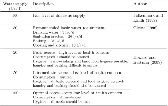
1.1 Domestic water supply levels of reference, in litres per capita per day (l/c/d). The figures 50 l/c/d and 100 l/c/d are used in the demand function. . . 14 1.2 Marginal willingness to pay (WTP) for the 100th _{litre per}

capita per day (l/c/d), calculated from the results of four econometric studies . . . 18 1.3 Marginal willingness to pay (WTP) at the bounds of the

blocks of the three-parts demand function, with LB: lower bound, UB: upper bound. . . 18 1.4 Calibrated maximum potential demand for the diﬀerent

coun-tries (where m3_{/c/y: cubic metre per capita per year; and}

l/c/d: litre per capita per day) . . . 21 1.5 Reconstructed current costs and prices of domestic water in

Mediterranean countries (around year 2000) . . . 23 1.6 Projected domestic demands in Mediterranean countries for

years 2010, 2025 and 2050, for the reference socioeconomic scenario . . . 26 1.7 Projection of total domestic water use at country scale,

com-parison with elements from the literature for four years of reference (km3_{/year) . . . .} ₃₆

1.8 Projections of total domestic water use at country scale for four years of reference: elements from the literature (km3_/year) ₃₈

2.1 Domestic and irrigation demands and values in Algerian basins. Comparison between modeled historical values and projec-tions at the 2050 horizon under various scenarios. Scenarios for the future are, for the domestic sector: F-med: Medium population variant & SSP2; F-high: High population variant & SSP5; F-low: Low population variant & SSP4. For agricul-ture: F-0: no crop prices increase; F-1: baseline crop prices increase scenario. . . 55 2.3 Data used for the computation of sugar beet price . . . 58

(15)

imisation and using one-point hedging (option V+_H+_{) . . . .} ₇₇

3.4 Impact of demand prioritisation: diﬀerence in satisfaction with the option V+_H+_{, compared to the results obtained with}

the option V H . . . 77 4.1 Examples of empirical studies that confirm the link between

climate change and migration . . . 98 4.2 Estimates and predictions of the overall number of migrants

related to global environmental change - adapted from Gemenne (2011) . . . 102 4.3 Definitions and concepts of "environmental migrants" used by

the main studies - adapted from Gemenne (2011) . . . 103 4.4 Examples of climate change induced migration modelling . . . 106 5.1 Notations . . . 116 5.2 Features of the New Economic Geography framework

pro-posed to consider water availability constraints, and compar-ison with Krugman’s seminal Core-Periphery model . . . 117 A.1 Vue d’ensemble des divers usages de l’eau . . . 150 A.2 Vue d’ensemble des méthodes d’évaluation non marchande les

plus utilisées . . . 157 A.3 Synthèse des valeurs de l’eau compilées pour diﬀérents usages

(16)

List of Figures

1 Population increase between 2000 and 2025/2050 in the main Mediterranean countries, according to UN projections [UN, 2009]. Bars represent the “Medium variant”, and error bars represent the “Low variant” and “High variant”. . . 2 2 Gross Domestic Product increase between 2000 and 2025/2050

in the main Mediterranean countries, according to OECD projections under the Shared Socioeconomic Pathway No.2 (Source: SSP database). . . 2 3 Countries of the Mediterranean basin . . . 3 1.1 General structure of the three-part inverse demand function

(with volumes Q and willingness to pay V ) . . . 13 1.2 Evolution of domestic water demand with economic

develop-ment: “structural change" modelling (with volumes Qbasic,

Qintand Qtot) . . . 14

1.3 Marginal willingness to pay along the demand curve, calcu-lated from the results of various econometric studies. In grey: econometric estimations using a log-log structural form, in black: linear structural form. Markers indicate the average observed levels of demand and price for each study. The dot-ted curve represents the demand function built for France, the pentagonal marker indicates the point of maximum po-tential demand calibrated for France and current water price in France. . . 17 1.4 Structure of the final three-parts inverse demand function and

its points of reference (volumes Q and values V ). Qbasic is set

to 50 l/capita/day, whereas Qintand Qtot depend on the level

of GDP per capita on the considered year. Qintand Qtotgrow

with GDP per capita with a saturation, their maximum value are respectively Maxint and Maxtot. Maxint is set to 100

l/capita/day, whereas Maxtot is calibrated at country scale. . 19

1.5 Projection of water demand and value over time for diﬀerent socioeconomic scenarios (reference scenario with a solid line, others with dotted lines), for a selection of countries. . . 25

(17)

1.9 Countries of the Mediterranean basin . . . 34 1.10 Total economic value of water: consumer’s surplus and water

utility’s revenue . . . 34 1.11 Calibration of the structural change curve for France, based

on historical domestic demand and GDP per capita. . . 35 1.12 Domestic water withdrawal projections (with reference

socioe-conomic scenario) compared to the literature, for Mediter-ranean countries with the highest levels of domestic with-drawal . . . 37 2.1 Modeling crop yield as a function of available water to ETc

ratio. Yirref and Yrfref are irrigated and rainfed crop yields of reference (in tons/ha), ET c is the crop evapotranspiration, pp the eﬀective precipitation. Irrigated crops are considered to be irrigated to the potential so, with W the quantity of irrigation water, by construction (pp + W )/ET c is always equal to one. 45 2.2 Domestic water demand function: economic development

ef-fect. Q1, Q2and Q3 are the volume limits of the three demand

parts. The gray arrows represent the eﬀect of economic de-velopment, which leads to larger demand by expanding the width of the blocks. . . 48 2.3 Domestic water demand function: surplus. D is the level of

demand corresponding to the level of price. The gray-colored area under the curve represents total economic surplus. . . . 49 2.4 Map of Algerian basins, labeled 1 to 15. Basins borders are in

black, and Algerian borders in white. The Mediterranean Sea is the white area. White dots represent cities of more than 100,000 inhabitants. Basin 2 is a basin located in western Algeria, that flows mostly through Morocco to the Atlantic Ocean and is out of the scope of this map. . . 51 2.5 Projected domestic and irrigation demands in Basin 4, for

year 2050, under the following scenarios: F-med (i.e. medium population variant and SSP2) for domestic demand, and F-0 (i.e. no price increase) for agricultural demand. . . 52

(18)

LIST OF FIGURES xv 2.6 Projected domestic and irrigation demands in Basin 1, for

year 2050, under the following scenarios: F-med (i.e. medium population variant and SSP2) for domestic demand, and F-0 (i.e. no price increase) for agricultural demand. . . 53 2.7 Projected domestic demand in basin 4, under historical

condi-tions for year 2000, and under three socioeconomic scenarios for year 2050. Scenarios: F-med (i.e. medium population vari-ant and SSP2), F-low (i.e. low population varivari-ant and SSP4) and F-high (i.e. high population variant and SSP5). . . 54 3.1 One-point hedging: one prudential parameter per reservoir

(↵), rationing is initiated when the stored volume is lower than Vlim . . . 73

3.2 Domestic water demand function: economic development ef-fect. Q1, Q2and Q3are the volume limits of the three demand

parts. The grey arrows represent the eﬀect of economic de-velopment, which leads to larger demand by expanding the width of the blocks. . . 81 3.3 Domestic water demand function: surplus. D is the level of

demand corresponding to the level of price. The grey-coloured area under the curve represents total economic surplus. . . . 81 3.4 Modeling crop yield as a function of available water to ETc

ratio. Yirref and Yrfref are irrigated and rainfed crop yields of reference (in tons/ha), ET c is the crop evapotranspiration, pp the eﬀective precipitation. Irrigated crops are considered to be irrigated to the potential so, with W the quantity of irrigation water, by construction (pp + W )/ET c is always equal to one. 83 3.5 Satisfying demands of each stream: downwards tree traversal,

with aggregations. (1) start with the most upriver streams, (2) aggregate upstream reservoirs’ system when moving down, (3) repeat until reaching the root of the network. . . 86 3.6 Distributing release between upstream reservoirs: upwards

tree traversal, with disaggregations. Steps for case (3) of Fig-ure3.5 . . . 86 3.7 Map of Algerian reservoirs systems. The white area is the

Mediterranean sea. Basins borders are in black. Light grey basins are basins without reservoirs. White triangles are reser-voirs, and white lines are the upstream-downstream links be-tween reservoirs. Numbered labels are located at the down-stream root of each system. . . 87 5.1 Coupling ODDYCCEIA to an economic geography model:

(19)

(20)

Remerciements

C’est avec le sourire que je parviens à cette ultime étape attendue avec tant d’impatience : les remerciements de thèse. Ça y est, c’est fini, et je tiens à saluer ici tous ceux qui ont contribué de près ou de loin à ce que je puisse écrire cette page.

Je remercie tout d’abord Jean-Charles Hourcade, pour m’avoir ouvert les portes du CIRED et m’avoir oﬀert les conditions administratives per-mettant mon inscription en thèse. Je remercie également la DGA pour son soutien financier à travers la bourse de thèse qu’elle m’a accordée, ainsi que le CIRED pour m’avoir accueillie en son sein, avec une pensée reconnaissante pour Christophe et Éléonore qui m’ont accompagnée à travers les vicissitudes administratives et budgétaires. Un grand merci à Patrice Dumas pour son encadrement, sa disponibilité et sa patience au cours de ces presque quatre années.

Je remercie également chaleureusement les membres du jury, les rappor-teurs Antonio Massarutto et Manuel Pulido Velázquez et les examinarappor-teurs Pascal Maugis, Jan Polcher et Philip Ward, pour avoir bien voulu consacrer du temps à l’évaluation de mon travail, ainsi que les membres de mon comité de thèse, Agnès Durcharne et Miren Lafourcade, qui ont permis une première confrontation salutaire de mon travail avec le monde extérieur.

Je souhaite également adresser mes remerciements à ceux rencontrés plus en amont sur le chemin de la thèse, mais dont le rôle n’en est pas moins important. En particulier Irène et Jean-Daniel qui, aux deux extrémités de mon cursus, m’ont mise sur de bonnes voies. Merci également à mon père pour m’avoir transmis sa curiosité et son esprit (trop) critique, et ma mère pour avoir eu suﬃsamment les pieds sur terre pour me permettre de survivre jusqu’à ce que je sois en âge de me nourrir seule.

Enfin, je souhaite exprimer toute ma gratitude à ceux qui m’ont accom-pagnée et soutenue tout au long de cette aventure initiatique.

Pour leur aide dans la dernière ligne droite, un grand merci à Fanny & Matt pour leurs relectures, à Vincent et Thierry pour leurs commentaires, ainsi qu’à tous ceux qui m’ont soutenue dans la préparation de la soutenance.

(21)

nommés mais qui ont participé à faire de ces années au Jardin Tropical une époque agréable. Une pensée aﬀectueuse également pour PatMat qui m’ont fourni ma dose hebdomadaire de protéines animales et viennoiserie.

Et comme la vie d’un thésard ne se passe pas uniquement au labo (hum), je remercie également mes deux tiers préférés pour leur amitié au long cours et leur précieuse singularité, Julien pour sa confiance en moi et sa joie de vivre communicative, et puis Aurore, Estelle, Etienne, Guillaume(s), Julie, Julien et tous les autres qui, ayant ou non eux-mêmes traversé l’épreuve de la thèse, ont su supporter mes jérémiades ou me les faire oublier.

(22)

Introduction

Global changes are expected to challenge the sustainability of water re-sources. Impacts of climate change on the hydrological cycle will add to non-climatic drivers of change such as demographic growth, economic devel-opment, land use changes, urbanisation etc. [Cisneros et al., 2014].

The issue is particularly acute in the Mediterranean region. On the one hand there is strong consistency in projections of reduced freshwater avail-ability in the Mediterranean region due to reduced rainfall and increased evaporation, and droughts are projected to become longer and more frequent [Cisneros et al., 2014]. On the other hand, demand is expected to increase with economic development and demographic growth (Figures 1 and2), es-pecially in countries of the southern and eastern Mediterranean rims (map in Figure3).

The Mediterranean is already a vulnerable area. More than half of the world’s “water-poor” population is located in the region, which concentrates 7.3% of the world’s population for only 3% of its water resources [Margat and Treyer, 2004].

Across the Mediterranean basin water supply and demand are charac-terised by an important spatial and temporal heterogeneity, related to the socioeconomic and hydroclimatic conditions. Demand is often higher in the summer months, when supply is lower. Potential total usable water resources vary from 113 m3_{/capita/year in Libya to almost 7000 m}3_{/capita/year in}

Greece. The sustainability of water resources is variable, with some re-sources being non-renewable. Total water use can represent less than 20% of the available renewable resources (e.g. Greece, France, Turkey) but it reaches 954% of renewable resources in Libya [Iglesias et al., 2007]. Water demand is also very variable. Among countries with the lowest use, some are con-strained by the lack of supply (e.g. less than 250 m3_{/capita/year in Malta or}

Algeria), while others use little water because they have little irrigated agri-culture (e.g. Croatia). In southern countries where irrigation is important (e.g. Egypt, Libya, Syria, Spain), water use per capita is the highest (over 1000 m3_{/capita/year in Egypt). At the basin level, situations can be even}

more contrasted [Margat and Treyer, 2004]. These heterogeneities could be accentuated or modified in the future through global changes.

(23)

Figure 1: Population increase between 2000 and 2025/2050 in the main Mediterranean countries, according to UN projections [UN, 2009]. Bars rep-resent the “Medium variant”, and error bars reprep-resent the “Low variant” and “High variant”.

Figure 2: Gross Domestic Product increase between 2000 and 2025/2050 in the main Mediterranean countries, according to OECD projections under the Shared Socioeconomic Pathway No.2 (Source: SSP database).

(24)

3

Figure 3: Countries of the Mediterranean basin

Water is an important factor of production for several sectors, agriculture in particular, and it is essential for human consumption. Spatially con-trasted situations, with some basins more aﬀected by water scarcity than others, could foster water related interactions between basins such as water transfers, virtual water trade, activity relocation, or migration. When facing water scarcity, people or activities could choose to relocate to a region where water is available. Changes in water availability could generate decreases in agricultural productivity, which could in turn exacerbate urban migration [Hallegatte et al., 2008].

Such inter-basin interactions could particularly arise in the Mediter-ranean. The region already engages in virtual water trade, the biggest net importer countries being Italy, Egypt, Spain and Algeria, mostly through crops trade. On the opposite, France is the biggest net exporter, through crops and livestock production exports [Margat and Treyer, 2004]. The re-gion also has a history of migrations between rims [de Haas, 2011].

These multi-basins issues are not often taken into account in policy mak-ing. Water scarcity is mostly contemplated from the basin scale, which is the usual water management level, with the perspective of reducing the demand-supply gap. The traditional response to tensions on water resources in the Mediterranean region has been to increase supply, by mobilising new resources (dams, groundwater, and more recently desalination) to meet the populations’ growing needs. As water resources become increasingly scarce, demand management policies are developed to limit losses and wastage in the use of the resource (through hydroeconomic equipment for instance).

(25)

This thesis contemplates the question of how heterogeneously distributed water constraints might foster inter-basin interactions in the Mediterranean region in the next decades, in particular in terms of economic activities and population mobility. For this, a proper representation of localised water constraints is needed.

The first objective of this thesis is thus to build a framework that can anticipate these localised water constraints.

This framework should project and compare future water supply and de-mand in each basin. Because of the nature of water’s specificities, this is a complex task. Surface water resources are mobile, and water availability downstream depends on upstream withdrawals. Some water uses are non-consumptive and generate return flows, while others consume all the water withdrawn. Demand and supply are variable in time and space, and they de-pend on various variables: climate, physical geography, socioeconomic con-ditions, etc. Water can be stored in reservoirs, which have an important impact on water fluxes [Biemans et al., 2011, Haddeland et al., 2013]. The Mediterranean region in particular is well equipped with dams. Water man-agement infrastructures were developed to regulate the variable flows, and distribute water to the demands when needed. At the beginning of the 21st

century, 1200 large dams (reservoirs of more than 10 million cubic meters) were in operation in Mediterranean countries, with 500 in the Mediterranean basin itself [Margat and Treyer, 2004].

The developed framework needs to adequately represent water manage-ment infrastructures, and how they allocate the available water between the diﬀerent uses in time and space. Water management policies are increas-ingly encouraged to consider water as an economic good [ICWE, 1992]. Wa-ter basin management requires being able to measure the economic benefits associated with water uses, and the changes in benefits associated with a change in water allocation or availability. In hydroeconomic models, water is allocated based on the economic benefits it generates. Hydroeconomic models address allocation between competing uses as well as inter-temporal allocation. The economically optimal allocation is the one that maximises

(26)

5 the aggregated economic value of the water used [Harou et al., 2009]. Know-ing the economic benefits associated with water use also makes it possible to estimate the potential direct economic losses associated with water short-age. Although economic rules are not often used in practice, water valuation could be used as a proxy for allocation policies in the absence of precise information on the priorities set between the diﬀerent demands in the diﬀer-ent basins. A hydroeconomic model could give localised water constraints in terms of quantities and in terms of direct costs for human activities.

The main challenge is that the framework must maintain a double focus: a large-scale coverage, and a representation of spatial heterogeneity at the river basin level. Indeed, on the one hand a large-scale coverage allows for the representation of interactions between basins with heterogeneous profiles; it also enables to address global changes and their impacts on water resources. On the other hand, water resources are managed at the river basin scale, and, depending on the river basin’s characteristics, the local impacts of global changes might be diﬀerent.

The extended geographic coverage will make it more complex to gather data to represent basscale characteristics: sectorial demands, water in-frastructure, etc. It will also make it difficult to take into account water value. Because markets are absent or inefficient for the water sector, it is not possible to directly observe the economic value of water. It is necessary to develop alternative non-market valuation techniques to reveal and esti-mate water’s value [Young, 2005]. These methods are data intensive, and difficult to implement on a large scale.

The approach developed in this thesis is generic hydroeconomic mod-elling: it aims at representing basin-scale heterogeneities as precisely as possible, while using only globally-available data, and keeping the model simple in order to limit computation time. It builds on the ODDYCCEIA framework [Nassopoulos, 2012], which was developed to study imbalances between water supply and irrigation water demand under climate change in the Mediterranean region.

The second objective of the thesis is to examine how the representation of localised water constraints could then be used to investigate their indirect impacts on economic activities and populations. While an overall reduction in water availability would constrain all activities, contrasted situations be-tween basins raise the more subtle question of interactions bebe-tween basins, in particular changes in activities and population locations. Localised con-straints on the resource could unsettle the organisation of human activities. To study this question, a framework representing the interactions be-tween water constraints and the organisation of the economy is needed. For instance, New Economic Geography studies the spatial organisation of the economy and represents why activities and people locate in one area or

(27)

an-and their direct economic costs, through the development of a large-scale hydroeconomic model. A first part is dedicated to the development of the demand side of the model. Chapter 1 focuses on projecting domestic de-mands and values, at country scale. Chapter 2 projects both domestic and irrigation potential demands and benefits; these projections are located in the diﬀerent basins, and associated with reservoirs. A second part concen-trates on the supply side of the model: Chapter3presents the reconstruction of reservoirs-demands networks, and the operation of water management in-frastructures.

The last part of the thesis contemplates using this large-scale hydroeco-nomic model to explore the indirect impacts of localised water constraints on economic activities location and population migration. Chapter4reviews literature on climate change induced migration, and Chapter5 proposes to investigate climate change induced migration through the lens of water avail-ability constraints, based on a New Economic Geography formalism.

AppendixAproposes an overview of concepts and methods for water val-uation, useful for readers who are not familiar with economic concepts.

(28)

Part I

Demand side:

projecting localised water

demands and values

(29)

(30)

Chapter 1

Projecting and valuing

domestic water use at regional

scale: a generic method applied

to the Mediterranean at the

2060 horizon

This chapter focuses on the demand-side of the water scarcity assessment, in particular on the domestic sector. It projects domestic demands and values at country scale. These demands will then be distributed between basins (Chapter2).

The chapter reproduces the contents of the following article: “Neverre, N. and P. Dumas (in press) Projecting and valuing domestic water use at regional scale: a generic method applied to the Mediterranean at the 2060 horizon. Water Resources and Economics.”

Abstract

The present work focuses on the demand side of future water scarcity assessment, and more precisely on domestic water demand. It proposes a quantitative projection of domestic water demand, combined with an original estimation of the economic benefit of water at large scale. The general method consists of building economic demand functions taking into account the impact of the level of equipment, proxied by economic development. The cost and price of water are assumed to grow with economic development.

The methodology was applied to the Mediterranean region, at the 2060 horizon. Our results show the evolution of water demand and value, measured by surplus, over time. As long as GDP per capita and water price remain low, demand per capita increases along with economic development, and surplus per capita increases with demand. As demand approaches saturation, the combined negative eﬀects

(31)

Pressure on water resources is a major issue in the Mediterranean region. More than half of the world’s “water-poor” population is located in the re-gion, which concentrates 7.3% of the world’s population for only 3% of its water resources [Margat and Treyer, 2004]. Global changes are expected to exacerbate this pressure on resources in the following decades: on the one hand water demand will increase with demographic growth and economic development, while on the other hand climate change is predicted to reduce water availability and intensify droughts around the Mediterranean [Barros et al., 2014].

Spatially contrasted situations, with some basins more aﬀected by water scarcity than others, could foster water related interactions between basins such as water transfers, activity relocations and, indirectly, migrations. Such interactions could particularly arise in the case of the Mediterranean, which has a history of exchanges and migrations between rims [de Haas, 2011].

In such a context, it is important to anticipate future water scarcity issues and identify basins at risk, in order to inform management strategies and policies. Traditionally, water management policies focused on adapting supply to demand, by mobilizing new water resources. But as resources become increasingly scarce and costly, policy makers have developed demand side management aiming at reducing water wastage.

In the present work we concentrate on the demand side of the water scarcity issue, and more precisely on domestic water demand. Irrigation is the largest water use sector in the Mediterranean, representing 63% of total water use [Margat and Treyer, 2004], and its projection is a research field of interest [Döll and Siebert, 2002]. However, its share in total water use is decreasing [Margat and Treyer, 2004]. Moreover, domestic demand, while accounting for a lower share of demand, is critical in terms of needs. Indeed, irrigation needs can be adjusted to some extent by virtual water trade, water scarce areas having the possibility of importing food rather than producing it themselves [Allan, 1997]. Domestic needs cannot be adjusted in that way. In addition, domestic uses such as consumption, food preparation and hygiene are essential to human life.

Some projections of domestic water use in Mediterranean countries exist, but they are not homogeneous between countries in terms of time horizons,

(32)

1.1. INTRODUCTION 11 methods and scenarios. In most cases they rely on simple trend prolon-gations [Margat and Treyer, 2004]. When looking at the whole region, a global projection methodology applicable to the diﬀerent countries, taking into account sociodemographic changes to come and simulating comparable scenarios across countries, is pertinent.

Generic global scale modelling of domestic water use is covered exten-sively in the literature [Alcamo et al., 2003b, Alcamo et al., 2007, Shen et al., 2008, Hanasaki et al., 2013a, Ward et al., 2010]. The general prin-ciple is to model and project a unitary water use intensity per capita, that is to be multiplied by the projected number of inhabitants. In the Water-GAP methodology [Alcamo et al., 2003a], the per capita water use intensity is modelled to evolve with the level of economic development (relationship statistically estimated at country scale) and decrease over time with tech-nological improvement (represented by a fixed rate of improvement). In the Total Runoﬀ Integrating Pathways (TRIP) model, future levels of domestic water use per capita in developing countries have been modelled either to converge towards that of present developed countries as economic growth continues [Shen et al., 2008, Hayashi et al., 2013], or independent of eco-nomic growth [Hanasaki et al., 2013a]. Other authors consider the impact of additional factors: Hughes et al. [Hughes et al., 2010] statistically estimate municipal water use per capita as a function of climatic variables and GDP per capita; Ward et al. [Ward et al., 2010] estimate municipal water demand as a function of GDP per capita and urbanisation rate, taking into account regional dummies and country characteristics as fixed eﬀects.

While evaluating water quantities at stake is essential, it is also relevant to have an idea of the economic benefits associated with water uses and the potential economic losses associated with water shortage. Economic valua-tion can be an indicavalua-tion on how to manage at best the available resource and allocate it between competitive uses when water is scarce. In hydroeco-nomic models, instead of considering water demands as fixed requirements, water is allocated to its diﬀerent uses based on the economic benefits it gen-erates: the economically optimal allocation is the one that maximises the aggregated economic value of the water used [Harou et al., 2009].

However, economic valuation of domestic water, as well as methods to project changes in water value, is absent from the large-scale literature. Be-cause markets are absent or ineﬃcient for the water sector, it is not possible to observe directly the economic value of water. It is necessary to develop alternative non-market valuation techniques to reveal and estimate water’s value [Young, 2005]. For the domestic sector, water is valued using willing-ness to pay and deriving economic surplus from econometric estimations of price-elasticity and demand functions [Young, 2005]. Such a method requires much data, which could be among the reasons explaining why hydroeconomic models have been developed mainly at an infra-national geographical scale [Harou et al., 2009].

(33)

domestic water demands at large scale and at a time horizon enabling to picture global changes (cf. diagram in1.A). Then it proposes an application to countries of the Mediterranean rim, from Western and Eastern Europe, Middle East and North Africa (cf. map of Mediterranean countries in1.B).

1.2 Building generic demand functions taking into

account structural change

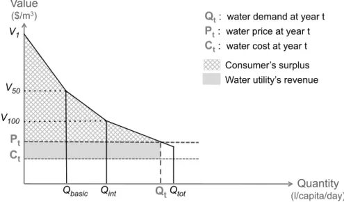
1.2.1 Overview

Our approach is to build simple three-part inverse demand functions (Figure 1.1), in which the willingness to pay for water decreases with quantity [Harou et al., 2009]. Each part of the demand function corresponds to a diﬀerent category of use. The first category corresponds to basic water requirements for consumption, food and hygiene, which are very highly valued (e.g. hand washing). The second category corresponds to intermediate needs, including additional hygiene (regular laundry, showers, etc.), less valued than uses of the first category. The last category corresponds to least-valued supplemen-tary consumption, such as further indoor uses (e.g. leisure bath) or outdoor uses (lawn watering, pool, fountain, etc.).

To build a demand function for each country, we determine the bounds of the demand blocks corresponding to these three categories: their respective volume limits (noted Q) and the marginal willingness to pay (noted V ) for those volumes.

Hence, the first step of the methodology is to determine the volume limits of the demand blocks, taking into account that demand will be impacted by economic development processes. The second step is to determine the willingness to pay for water at those volumes of reference, in order to value water. This second step also makes it possible to take into account the possible impact of water price on demand.

(34)

1.2. METHODOLOGY 13 V₂ V₀ Q₁ Q₂ Q₃ Value ($/m3₎ Quantity (l/capita/day) V₃ V₁

Figure 1.1: General structure of the three-part inverse demand function (with volumes Q and willingness to pay V )

1.2.2 Volumes of the demand blocks: taking into account structural change

Following Alcamo et al. [Alcamo et al., 2003a] and their “structural change" modelling, we want to take into account that average domestic water de-mand per capita grows along with economic development, proxied by GDP per capita, in order to take into account equipment eﬀects. Indeed, as their income increases households get more water-using appliances (washing ma-chines, dishwasher, etc.) and use more water; eventually they reach equip-ment saturation and water use stabilises whilst income continues to grow. To take into account structural change, we consider that the volumes of the blocks of our demand function evolve over time following economic develop-ment.

We assume that only non-essential uses are sensitive to this equipment ef-fect, so we consider that the volume of the first block of our demand function is fixed. Following Gleick [Gleick, 1996] and Howard and Bartram [Howard and Bartram, 2003] (Table1.1), we set the volume limit of the first demand block to 50 l/c/d, which meets needs for consumption, food and personal hygiene.

The volumes of the second and third demand blocks are assumed to evolve with the level of GDP per capita, with a saturation, drawing a sigmoid curve (Figure1.2). When GDP per capita is low, water demand is composed of only basic uses and intermediate uses (categories 1 and 2); intermediate uses grow with economic development. Then, as GDP per capita further increases, third category uses appear and the third demand block grows along with the intermediate demand block. Eventually, demand reaches saturation and stabilises.

(35)

Drinking water : 5 l/c/d Sanitation services : 20 l/c/d Bathing : 15 l/c/d

Cooking and kitchen : 10 l/c/d

20 Basic access - high level of health concern Consumption : should be assured

Hygiene : hand-washing and basic food hygiene possible; laundry and bathing diﬃcult to assure

Howard and Bartram (2003) 50 Intermediate access - low level of health concern

Consumption : assured

Hygiene : all basic personal and food hygiene assured; laundry and bathing should also be assured

100 Optimal access - very low level of health concern Consumption : all needs met

Hygiene : all needs should be met

Q_basic Demand (l/capita/day) block 3 block 2 block 1 Q_tot Q_int Economic development (GDP/capita) M_tot+Q_basic M_int+Q_basic Q_basic ftot f_int

Figure 1.2: Evolution of domestic water demand with economic development: “structural change" modelling (with volumes Qbasic, Qint and Qtot)

(36)

1.2. METHODOLOGY 15 the sigmoid function ftot:

Qtot = ftot(GDP ) = mtot+ Mtot.[1 exp( tot.GDP2)]

The function ftot is defined by three parameters: the minimum demand

(mtot), the maximum additional demand (Mtot) and the curve parameter

( tot); GDP stands for average GDP per capita. Parameter mtot is set to

match basic needs: mtot = Qbasic= 50 l/c/d. The two remaining

param-eters of ftot are to be statistically estimated at country scale using GDP,

population and domestic water demand data (Section 1.3.1).

Then, to distinguish between second-block and third-block volumes, we introduce the following sigmoid curve fint:

fint(GDP ) = mint+ Mint.[1 exp( int.GDP2)]

This curve fint is defined only starting from its intersection with ftot, noted

(GDP°_{, Q}°_{). Before this wealth level GDP}°_{, demand of the third category}

is null; after, intermediate demand is: Qint = fint(GDP ), and demand of

the third category is: Qtot Qint (Figure1.2).

Parameters of fint are completely determined without need for a

statis-tical estimation. First, we set: mint= Qbasic= 50 l/c/d. Then Mint is set

so as to match the reference figures of a “fair level of domestic supply" from the literature [Falkenmark and Lindh, 1993, Howard and Bartram, 2003]: Mint+ mint= 100 l/c/d (Table 1.1). Finally, we constrain fint by setting

its inflection point so as to belong to the curve ftot, which determines int.

Once structural change curves parameters are calibrated for a chosen country, the volumes of the blocks of its demand function can be determined for a given year depending on the level of GDP per capita (Figure1.2).

1.2.3 Willingness to pay for water along the demand function

Once the volumes of water demand are determined, we estimate the will-ingness to pay (WTP) for water along the demand function. The following section describes how we determine the WTP at the lower and upper bound volumes of each category (i.e. 1st_{, 50}th _{and 100}th _{l/c/d, and maximum}

po-tential demand), then interpolate linearly.

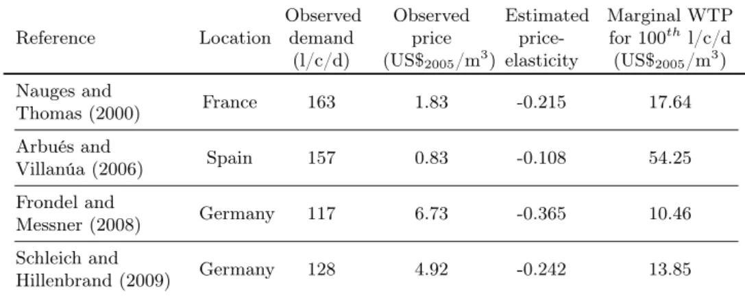
We collected econometric studies, located in the Mediterranean region or in Europe, that estimate the response of domestic water demand to price. Studies that provided both estimated price elasticities and observed levels of price and demand were used to calculate the marginal willingness to pay for water along the demand curve for each study, following the point-expansion method [Harou et al., 2009]. Demand values were adjusted for some studies [Arbués and Villanúa, 2006,Frondel and Messner, 2008,García-valiñas, 2005, Martínez-Espiñeira, 2002,Martínez-Espiñeira, 2003,Martins and Fortunato,

(37)

mand (369 l/c/d) for a higher price (1.64 $2005/m3). Some studies performed

the econometric estimation with a linear structural form [García-valiñas, 2005,Martínez-Espiñeira, 2002,Martínez-Espiñeira, 2003,Martins and For-tunato, 2005] , others with a log-log structural form (i.e. constant price-elasticity) [Arbués and Villanúa, 2006, Frondel and Messner, 2008,Nauges and Thomas, 2000,Schleich and Hillenbrand, 2009]. The linear studies led to low slopes, with a very low WTP for water for the first litre consumed (1.59-4.98 $/m3_{), and WTP in the [0.57 $/m}3_{; 4.09 $/m}3_{] range for the 100}th

l/c/d [García-valiñas, 2005, Martínez-Espiñeira, 2002, Martínez-Espiñeira, 2003,Martins and Fortunato, 2005].

For low demand levels, the linear structural forms are likely to underes-timate water values since esunderes-timates are much lower than prices actually paid for (e.g. bottled water, which can reach 300 $/m3 _{or higher). Moreover, such}

low values do not agree with the notion that water is essential [Arbués et al., 2003]. Values given by log-log structural forms are higher, but the econo-metric estimations were performed in conditions where observed demands were higher than 100 l/c/d. For low demand levels, i.e. the 1st _{and 50}th

l/c/d, which are far from the observations range of the estimations, we chose not to rely on econometric estimates of WTP for water and made simple assumptions (Table1.3).

For the 100th _{l/c/d, values given by the linear form are much lower than}

values obtained with log-log structural form. Even though there is no strong evidence that the values given by the linear form are incorrect, we assumed that values were too low at this demand level. Therefore, we chose to rely only on the marginal WTP for water calculated from studies using a log-log structural form. Three studies remained, after we chose not to use the results derived from Arbués and Villanúa [Arbués and Villanúa, 2006], for which a high observed demand combined with a low price-elasticity implies a steeper slope and much higher values than the other studies (Figure1.3 and Table 1.2). Demand consists of total domestic demand (i.e. residential uses and collective uses).

The marginal WTP for the 100th_{l/c/d ranges from 10.46 to 17.64 $/m}3_,

with a 25% variation range around the average of 14. We assume that the WTP for the 100th _{l/c/d is 14 $/m}3_{. Because the error range of this}

(38)

1.2. METHODOLOGY 17

Figure 1.3: Marginal willingness to pay along the demand curve, calculated from the results of various econometric studies. In grey: econometric es-timations using a log-log structural form, in black: linear structural form. Markers indicate the average observed levels of demand and price for each study. The dotted curve represents the demand function built for France, the pentagonal marker indicates the point of maximum potential demand calibrated for France and current water price in France.

parameter is high, it is included in the sensitivity analysis performed in Section1.4.

For the upper bound of the third block, we use available data on cur-rent water price. Combining observed quantity and observed price could give us a point of the demand curve. However, if equipment limits demand, there is some rationing and the point of observed demand does not corre-spond to the consumption level where willingness to pay equals price and consumer’s marginal surplus becomes null. To estimate this level of de-mand, unconstrained by equipment, we use the maximum potential demand Qbasic+ Mtot, i.e. the plateau of the structural change function ftot. Hence

we use Qbasic + Mtot and Pt=0 as a reference point of the demand curve,

where Pt=0is the current water price, determined by the authors from

avail-able data (Tavail-able 1.5 and Section 1.3.2). This point constitutes the upper bound of the third category demand block (Table 1.3). Then, for a given year, the third block actually ends when reaching Qtot, i.e. the actual total

(39)

Frondel and

Messner (2008) Germany 117 6.73 -0.365 10.46

Schleich and

Hillenbrand (2009) Germany 128 4.92 -0.242 13.85

Table 1.3: Marginal willingness to pay (WTP) at the bounds of the blocks of the three-parts demand function, with LB: lower bound, UB: upper bound.

Volume Marginal WTP _{Justification}

Point of reference l/capita/day US$2005/m3

LB block 1 1st ₃₀₀ _{Average price of bottled water}

UB block 1: Qbasic 50th 50 Assumption

UB block 2: Qbasic+Mint 100th 14 Adapted from literature

(Sec-tion1.2.3)

UB block 3: Qbasic+Mtot country specific Pt=0 Point of maximum potential demand if equipment was not limiting

demand for the level of GDP per capita of the considered year, as demand is constrained by revenue and domestic equipment (Figure1.4).

Table 1.3 summarises the figures used to define the WTP for water at the bounds of the blocks of our three-part inverse demand function. Once the WTP for water at the volume points of reference of the three categories of demand has been determined, a linear interpolation is used to build the demand function. The linear form is chosen for its simplicity, in absence of data justifying another shape.

In this way, we build a domestic demand function for each country, whose parameters take into account the impact of economic development on de-mand. The structure of that final demand function is pictured in Figure1.4, where Qintand Qtotare being redetermined for each year following projected

GDP per capita. The total economic value of the water used can be derived from this demand function, depending on the cost of water, the price of water and the level of satisfaction of the demand: it consists of consumers’ surplus plus the water utility’s revenue (1.C). Water utility’s revenue can be

(40)

1.3. APPLICATION TO THE MEDITERRANEAN REGION 19

V₁₀₀ P_t=0

Q_basic Q_int Q_tot Max_tot

V₅₀ Value ($/m3₎ Quantity (l/capita/day) Max_int Q_basic= 50 l/capita/day

Max_int= 100 l/capita/day

Max_tot= Q_basic+ M_tot Q_int= f_int(GDP) ≤ Max_int Q_tot= f_tot(GDP) ≤ Max_tot V₁= 300 $/m3

V₅₀= 50 $/m3

V₁₀₀= 15 $/m3

P_t=0= current price

V₁

Figure 1.4: Structure of the final three-parts inverse demand function and its points of reference (volumes Q and values V ). Qbasicis set to 50 l/capita/day,

whereas Qintand Qtot depend on the level of GDP per capita on the

consid-ered year. Qint and Qtot grow with GDP per capita with a saturation, their

maximum value are respectively Maxint and Maxtot. Maxint is set to 100

l/capita/day, whereas Maxtot is calibrated at country scale.

negative if price is lower than cost.

A sensitivity analysis is later carried out to assess the impact of the diﬀerent assumptions (Section1.4).

1.3 Application to the Mediterranean region

The first step is to calibrate structural change curves for each country. Then, for a given year t and level of GDP per capita GDPt, potential intermediate

and total demands can be determined and used to define the volumes of the blocks of the three-part demand function for year t (Figure 1.4). Finally, actual demand for year t can be determined depending on the price of water Pt.

1.3.1 Calibration of structural change curves for the Mediter-ranean countries

Structural change curves parameters (M and , Cf. Section 1.2.2) were cal-ibrated for countries of the Mediterranean rim based on data available at a regional scale. Historical water demands were determined using water with-drawal data at country level from the Mediterranean Information System on

(41)

ilarities1 _{need to be made. For Montenegro, we used the plateau calibrated}

on Greece. For the remaining countries, in absence of a suitable country of reference, we set the maximum additional demand parameter (Mtot) and

pricing (Pt=0) to the average value in countries where it could be estimated,

and calibrated only the curve parameter ( tot). For Montenegro, we did not

have suﬃcient data to fit the curve parameter either, so we used the curve parameter calibrated on Greece.

Results of the calibration of the Mtot parameter and resulting maximum

potential demands for each country are presented in Table1.4. The plateau level is the lowest in Malta and France, and the highest in Spain and Italy. Goodness of fit between country data and the obtained calibrated function is evaluated with Willmott index of agreement in its original form [Willmott, 1981], which is suitable for sigmoid curves. For France, the curve fits well visually (1.D), but in this specific case the Willmott index is not an appro-priate indicator of goodness of fit because historical consumption has already reached the plateau and observations are flat (instead of being of a sigmoid form), so the sum of squares of the regression (SSR) is null.

In our methodology the projection variable is demand, leaving the pos-sibility of making various assumptions about the evolution of network ef-ficiency when determining the corresponding withdrawal. To be able to compare our calibration results with those of the WaterGAP methodology applied to European countries [Flörke and Alcamo, 2004], we converted our demand figures into withdrawals under the assumption that demand to with-drawal ratios remain equal to current ratios (average current ratios, adapted from Margat and Treyer [Margat and Treyer, 2004], cf. Table1.6). For Spain and Slovenia, our results are very similar to Flörke and Alcamo [Flörke and Alcamo, 2004] findings, with less than 10% of difference in maximum poten-tial withdrawals, whereas for France and Italy we obtain substanpoten-tially lower results (-65 to -85%). Flörke and Alcamo [Flörke and Alcamo, 2004] perform their structural change calibration using adjusted data: they offset past im-provements in water use efficiency by applying a fixed annual technological 1_{Maximum potential demands should reflect cultural effects, along with other factors} influencing domestic water demand (climate, household characteristics, etc.).

(42)

1.3. APPLICATION TO THE MEDITERRANEAN REGION 21 Table 1.4: Calibrated maximum potential demand for the diﬀerent countries (where m3_{/c/y: cubic metre per capita per year; and l/c/d: litre per capita}

per day)

Country Mtot parameter Maximum potential demand Willmott index of agreement (m3_/c/y) _(m3_/c/y) _(l/c/d) France 54.52 72.77 199 0.00 Israel 71.79 90.04 247 0.41 Italy 92.11 110.36 302 0.63 Malta 54.49 72.74 199 0.65 Slovenia 82.08 100.33 275 0.44 Spain 91.26 109.51 300 0.83 Othersa _77.58 _95.83 ₂₆₃

-a_{Albania, Algeria, Bosnia, Croatia, Cyprus, Egypt, Greece, Lebanon, Libya,} Morocco, Syria, Tunisia, Turkey, Montenegro

change rate. The adjusted data they use are therefore higher than historical data, which can explain the diﬀerences with our results for France and Italy. For Malta, Flörke and Alcamo [Flörke and Alcamo, 2004] obtained a very low plateau (about two times lower than ours), which could be because their data do not take into account desalinated water.

1.3.2 Projection scenarios

The calibrated three-part demand curves were used for the projection and valuation of domestic water demands in the Mediterranean countries, as a function of economic development and water price. Since demands are mostly higher than the upper bound of the second block (100 l/c/d), for simplification we used the average value of water per block instead of the variable marginal value in the first two blocks of the demand functions when calculating consumer’s surplus. This could lead to an underestimation of consumer’s surplus when demand is lower than 100 l/c/d (Morocco before year 2010, Bosnia before 2015, Tunisia before 2020, Algeria until 2050 under the reference scenario).

Projection and valuation of future domestic water demands at the 2060 horizon were performed under contrasted scenarios of economic development and population growth. For economic development scenarios, we used GDP projections of the five Shared Socioeconomic Pathways (SSPs) [Rozenberg et al., 2014] available in the SSP Database (version 0.9.3). For population projections, we used four UNO scenarios: the medium, low and high variants, and the constant fertility variant. The medium population variant combined with the SSP2 economic scenario is used as the reference scenario.

The cost of water was assumed to evolve over time as countries develop and invest in water infrastructures. Current cost level in France was

(43)

cho-capita in France.

For Malta, the particular context of the water sector implies a very high cost of water due to intensive desalination: 62% of the water used came from desalination in 1998-1999 [Margat and Treyer, 2004]. For Croatia, the current cost of water is also above the target cost level. Therefore, no further increase in water cost was projected for Malta and Croatia.

The cost-recovery ratio was assumed to converge towards one as GDP per capita grows, reaching one when GDP per capita reaches the current level of GDP per capita in France. The price of water changes over time, resulting from the combination of cost evolution and cost-recovery evolution. Current water prices and costs in each country were not directly avail-able, they had to be reconstructed using available data on water costs or prices from Margat and Treyer [Margat and Treyer, 2004], OECD [OECD, 2010] and International Benchmarking Network for Water and Sanitation Utilities database (IBNET [International Benchmarking Network for Water and Sanitation Utilities, 2013]), cost-recovery ratios from Margat and Treyer [Margat and Treyer, 2004], Euro-Mediterranean Water Information System database (EMWIS [Euro-Mediterranean Water Information System, 2013]) and IBNET, and sewerage coverage ratios from EMWIS and IBNET. Domes-tic water prices and costs are estimated with two diﬀerent methods: using available data on prices and costs, or reconstructing costs based on the most robust data and sewerage coverage rates. Then the maximal value given by these two methods is selected, to avoid unrealistically low values.

For the first method, in a first step data on water prices and costs are deflated. When possible, missing costs are determined using the cost/price ratio in each country. If this information is not available, the water volumes weighted average Mediterranean cost/price ratio is used (using SIMEDD data for year 2000 water volumes). The obtained values are then multiplied by a 1.3 factor to take into account additional costs (other than operational costs). The 1.3 figure originates from data on France from Margat and Treyer [Margat and Treyer, 2004]. Robust water costs data are available for four countries (France, Greece, Italy and Spain), the minimum estimated costs are observed for Italy (2.17$/m3). This minimum cost accounts for both water services and sanitation services, each representing 50% of this cost.

(44)

1.3. APPLICATION TO THE MEDITERRANEAN REGION 23 Table 1.5: Reconstructed current costs and prices of domestic water in Mediterranean countries (around year 2000)

Country _(US$2005/mCost 3₎ _(US$2005/mPrice 3₎ Years of available data

Albania 1.79 0.93 <2004, 2011

Algeria 2.01 0.41 <2004, 2010

Bosnia and Herzegovina 1.68 0.93 2007

Croatia 4.33 2.55 <2004 Cyprus 2.62 1.33 1989, <2004 Egypt 1.63 0.16 1989, <2004, 2010 France 3.33 3.33 <2004, <2010 Greece 2.22 1.31 <2004, <2010 Israel 2.15 0.95 <2004, <2010 Italy 2.17 1.4 1994, <2004, <2010 Lebanon 2.05 1.2 1989, <2004

Libyan Arab Jamahiriya 1.84 0.09 1997, <2004

Morocco 2.05 1.04 1989, <2004

Malta 10.58 2.08 <2004

Montenegro 1.65 0.93 2012

Slovenia 2.81 1.66 <2004

Spain 2.75 1.62 <2004, <2010

Syrian Arab Republic 2.83 0.91 1989, <2004

Tunisia 1.9 0.91 1989, 1996, <2004, 2010

Turkey 2.1 1.17 <2004, 2008

We use this value as a basis to calculate minimum costs for all the other countries in the second method.

For the second method, we estimate a minimal domestic water cost de-pending on the sewerage coverage rate. For countries where robust water costs data are not available, we assume that water distribution services costs are 2.17/2 $/m3 _{(i.e. half of the minimum total cost among countries with}

robust data). We then add sanitation costs, which vary from 0 to 2.17/2 $/m3_{, depending on the sewerage coverage rate.}

Final cost and price data used are displayed in Table 1.5.

1.3.3 Projection results

Results of projected water demand per capita are presented in Figure1.5for a selection of countries and in Table 1.6. Developed countries have mostly reached demand saturation: demand per capita does not increase in France, Israel and Malta, and it increases by only 2.1% to 9.7% in Spain between 2000 and 2060 under the diﬀerent scenarios. In contrast, demand per capita grows sharply in developing countries, at a pace depending on socioeconomic drivers. In Egypt, domestic water demand per capita is of 45.36 m3_{/c/y in}

2000, and it grows rapidly and reaches potential demand around 2030-2035 (Figure 1.5(a)). In Morocco and Algeria, initial demand is lower

(45)

(respec-increases with economic development, and surplus per capita (respec-increases with demand. Eventually, when GDP per capita and price reach a certain level, demand per capita begins to saturate and decrease, which impacts surplus negatively. In parallel, as the country develops the cost of water increases, which also impacts surplus negatively. As a result, surplus per capita be-gins to decrease sooner than demand per capita. The negative net eﬀect on surplus is visible for Egypt, Israel, Morocco, Spain and Turkey (Figure 1.5(b)).

Malta is a particular case. The cost of water is the highest among Mediterranean countries: 10.58 $2005/m3 compared with an average cost

of 2.77 $2005/m3 in the other countries. Surplus is particularly low due to

this high cost of water. The impact of price on demand per capita is more pronounced for Malta (-35.7% in 2060) than for other countries, as the price of water converges towards a higher cost.

Total demand at country scale is the result of demand per capita evolu-tion and populaevolu-tion growth. In some countries, such as Turkey and Egypt, the combination of a strong population growth and increase in individual wa-ter demand leads to a rapid rise of total wawa-ter demand: +170% for Turkey and +210% for Egypt between 2000 and 2030, under the reference scenario (Figure 1.5(c)). In other countries, such as Algeria, demand per capita re-mains limited by revenue constraints and so, despite a high population in-crease, total demand does not grow that sharply in the first decades: +110% between 2000 and 2030 under the reference scenario. By 2060, total demand could almost triple under the reference scenario: +186% in Turkey, +273% in Egypt, and +286% in Algeria (compared with year 2000).

We compared our results with domestic water use projections in Mediter-ranean countries available in the literature (1.E). Globally our projections fall in the range of existing figures, which can be wide for non-OECD countries.

1.3.4 Simulation of a strong cost increase scenario

Under the standard price evolution modelled in Section 1.3.3 (Malta not included), the eﬀect of price increase leads to a decrease in demand of up to 10.9% in 2060. These results were obtained under the assumption that

(46)

1.3. APPLICATION TO THE MEDITERRANEAN REGION 25

(a) Demand per capita

(b) Surplus per capita (consumer surplus + water utility revenue)

(c) Total domestic water demand at country scale

Figure 1.5: Projection of water demand and value over time for diﬀerent socioeconomic scenarios (reference scenario with a solid line, others with dotted lines), for a selection of countries.

(47)

Table 1.6: Projected domestic demands in Mediterranean countries for years 2010, 2025 and 2050, for the reference socioeconomic scenario

Country Total demand Demand per capita Demand towithdrawal

ratios (%)a

(km3_/y) _(m3_/c/y)

2010 2025 2050 2010 2025 2050

Albania 0.30 0.32 0.28 93.49 95.72 93.21 45

Algeria 0.83 1.22 2.03 23.52 29.04 43.57 50

Bosnia and Herzegovina 0.13 0.21 0.27 35.63 59.01 89.79 40

Croatia 0.31 0.35 0.33 69.97 83.3 84.73 67.5 Cyprus 0.07 0.08 0.12 61.54 64.57 86.39 77 Egypt 4.86 8.78 11.35 59.93 86.96 91.96 52.5 France 4.57 4.89 5.27 72.77 72.77 72.77 70 Greece 0.81 0.91 1.05 71.6 78.45 89.79 66.5 Israel 0.64 0.74 0.96 86.39 80.22 80.22 81.5 Italy 6.21 6.05 5.86 102.64 98.99 98.99 73 Lebanon 0.34 0.44 0.42 80.68 94.44 89.79 65 Libya 0.55 0.7 0.79 87.06 93.94 89.79 75 Malta 0.03 0.02 0.02 67.69 46.74 46.74 65 Montenegro 0.02 0.03 0.05 32.74 44.38 74.59 63 Morocco 1.31 2.67 3.6 41.07 73.28 91.81 78.5 Slovenia 0.17 0.19 0.18 85.44 91.64 91.64 67.5 Spain 4.36 4.92 5.1 94.61 99.47 99.38 70 Syria 1.25 2.33 3.05 61.18 89.56 92.24 72.5 Tunisia 0.33 0.61 1.14 31.58 51.29 89.79 69 Turkey 4.11 6.92 8.23 56.5 82.37 89.79 50