Flicker Removal and Color Correction for High Speed Videos

(1)

HAL Id: tel-01744714

https://pastel.archives-ouvertes.fr/tel-01744714

Submitted on 27 Mar 2018

HAL is a multi-disciplinary open access archive for the deposit and dissemination of sci-entific research documents, whether they are pub-lished or not. The documents may come from teaching and research institutions in France or abroad, or from public or private research centers.

L’archive ouverte pluridisciplinaire HAL, est destinée au dépôt et à la diffusion de documents scientifiques de niveau recherche, publiés ou non, émanant des établissements d’enseignement et de recherche français ou étrangers, des laboratoires publics ou privés.

Flicker Removal and Color Correction for High Speed

Videos

Ali Kanj

To cite this version:

Ali Kanj. Flicker Removal and Color Correction for High Speed Videos. Other [cs.OH]. Université Paris-Est, 2017. English. �NNT : 2017PESC1115�. �tel-01744714�

(2)

École Doctorale Mathématiques et Sciences et Technologies de l’Information et de la Communication

Thèse présentée pour l’obtention du titre de

Docteur en Traitement du Signal et des Images

Flicker Removal and Color Correction for High

Speed Videos

par

Ali KANJ

à soutenir le devant le jury composé de

Rapporteur Fréderic DUFAUX

Rapporteur Fabrice MERIAUDEAU

Examinatrice Julie DELON

Examinateur Etienne DÉCENCIÈRE

Examinateur Raoul RODRIGUEZ LUPARELLO

Directeur de Thèse Hugues TALBOT

Co-Directeur de Thèse Jean-Christophe PESQUET

(3)

(4)

Abstract

Deflickering consists of removing rapid, artifactual changes of luminosity and colorimetry from image sequences and improving luminosity consistency between video frames. It is a necessary and fundamental task in multiple applications, for instance in archived film sequences, compressed videos and time-lapse videos. In recent years, there has been a renewal of interest for improving luminosity consistency acquisition technology in the flicker removal problem, in particular for periodic flickering. In this context, flicker corresponds to undesirable intensity and chroma variations due to the interaction between the acquisition frequencies on the one hand, and the alternating current powering the light sources on the other hand. The present thesis formulates the periodic deflickering problem in high speed videos, studies the physical properties of flicker and suggests both theoretical and experimental solutions for its removal from image sequences. Finally, a new flicker removal approach is proposed performing jointly motion tracking and color correction.

Résumé

Le deflickering consiste à supprimer le scintillement présent dans les séquences d’images afin de réduire les variations lumineuses entre chacune des images de la vidéo. Il s’agit d’une tâche essentielle, nécessaire dans plusieurs applications, en particulier dans les séquences de films archivés, les vidéos comprimées et les vidéos time-lapse. Au cours de ces dernières années, avec le développement des technologies d’acquisition à haute vitesse, il y a eu un regain d’intérêt pour le problème de suppression de flicker, en particulier le flicker périodique. Dans ce contexte, le flicker correspond à des variations indésirables de luminosité et des couleurs dues à l’interaction entre la vitesse d’acquisition d’une part, et d’autre part le courant alternatif alimentant les sources lumineuses. La présente thèse formule le problème du déflickering périodique dans les vidéos à haute vitesse, étudie les propriétés physiques du flicker et propose à la fois des solutions théoriques et expérimentales pour sa suppression des séquences d’images. Enfin, une nouvelle approche est proposée permettant d’effectuer simultanément le suivi de mouvement et la correction des couleurs.

(5)

(6)

Acknowledgements

I would like to thank the members of the jury, for they have accepted to assess the present thesis: Fréderic Dufaux, Fabrice Meriaudau, Julie Delon, Etienne Décencière.

Hugues Talbot and Jean-Christophe Pesquet were my phd advisors during the last three years. They accepted me first as a research trainee and then as a phd candidate, they encouraged me to think freely. I am grateful for their availability and expertise. I am thankful for their patience, positivity and open-mindedness. I would like to thank SUBLAB Production, represented by Raoul Rodriguez Luparello, for funding this phd studies.

The LIGM lab members accepted me amongst them. I thank them for their welcome and for their cheerful mood and for the good memories we share.

(7)

(8)

List of Figures

2.1 Bayer filter . . . 13

2.2 Chronophotography: First high speed sequence . . . 14

2.3 High speed imaging examples . . . 15

2.4 Rugby action in slow motion. . . 16

2.5 The use of high speed imaging in advertising photography . . . 16

2.6 Comparison between several types of flicker . . . 22

2.7 Chroma alterations with light temperature variations . . . 24

2.8 Rapid illumination / chromatic changes in a high-speed video sequence.. . . 24

2.9 Illumination / chromatic changes in a high-speed video sequence under fluorescent lighting. . . 25

2.10 The blue curve shows the luminosity variation in an affected image sequence. In red we show the intensity variation in the absence of periodic flicker. . . 26

2.11 Cross-channel correlation between a flicker-affected frame and a reference image.. . . 27

3.1 Phase correlation example Zitova and Flusser (2003): the graph on the left depicts red-red channel matching and the right one demonstrates red-blue channel matching. The peaks correpond to the matching positions. . . 33

3.2 Classical variational methods for motion estimation between two images with illumination constancy.. . . 41

(15)

xiv List of Figures

3.3 Classical variational methods for motion estimation between two images acquired from a naturally lit scene with a slight additionnal

arficial flicker . . . 41

3.4 Farnebäck optical flow method: the first row corresponds to the plots of some samples of motion vectors. Images in second row show the motion vectors in HSV space, and present the direction (corresponding the hue value) and magnitude (corresponding to the lightness value ) on motion vectors. . . 42

3.5 Block matching using the mutual information criterion, (b) is the reference frame manually shifted for few pixels, (c) shows motion vectors of blocks from the reference frame to the target frame. . . 46

3.6 Test on the car sequence: the horizontal motion of the car is well estimated, but it fails on some homogenous regions. It is recommended to increase the block size in order to include more texture information. . . 47

3.7 Global color transfer example: Basing on the paper of Reinhard et al. (2001), this method requires only the mean and standard deviation of pixel intensities for each channel in the L*_a*_b* _color space. The transfer fails to resynthesise the colour scheme of the target image. . . 49

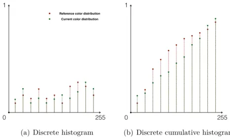
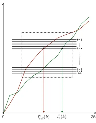
4.1 An example of the computation of the discrete cumulative his-tograms to present the color distributions in two images. . . 56

4.2 An example of the matching between different data sets in discrete and interpolated cumulative histograms . . . 56

4.3 lc ref vs. lct.. . . 58

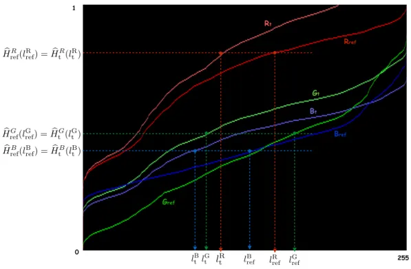
4.4 The choice of data sets samples from the central part of histograms. 59 4.5 The normalized cumulative histograms representing the color dis-tribution of three color channels in the reference and target frames f(⋅, t_ref) and f(⋅, t). . . . 61

4.6 Falcon sequence with global artificial flicker . . . 62

4.7 Falcon sequence with local artificial flicker . . . 63

(16)

List of Figures xv

4.9 Real flickering sequence 1 . . . 64

4.10 Real flickering sequence 2 . . . 64

4.11 Scale space construction: Gaussian pyramid . . . 70

4.12 DoG pyramid . . . 71

4.13 Vertical vs. horizontal translations of matched keypoints . . . 73

4.14 Vertical vs. horizontal translations of matched keypoints with Euclidean distance . . . 74

4.15 Random sampling on the image . . . 75

4.16 Image sequence with periodic flicker from studio lighting. . . 77

4.17 Global color correction using image registration based method . . 77

4.18 A comparison between luminosity average before and after flicker correction using image registration based method . . . 78

4.19 Sequence with global motion and artificial flicker. . . 79

4.20 Artificial flicker: similarity measures . . . 80

5.1 An illustration of flicker effects in different regions of a single sequence. Luminosity variations vary significantly between regions, and so cannot be corrected in the same way everywhere. . . 82

5.2 Illustration of MM algorithm for the minimization of a function g∶ RN →]−∞, +∞]. At iteration k ∈ N, we use a majorant function q(⋅ ∣ uk) of g at a point uk, and then we define uk+1 as a minimizer of q(⋅ ∣ uk). . . 86

5.3 Block matching scheme . . . 90

5.4 The convergence of our iterative algorithm depends of the param-eters initialization. This test was performed on an image for the Bird sequence. . . 92

5.5 Huber norm: The PSNR of the processed image for the Bird sequence while increasing ε. . . . 93

5.6 Similarity comparison: PSNR average of the processed sequence using different cost functions. The sequence is acquired with large local motion and a periodic artificial flicker has been added. . . . 96

(17)

xvi List of Figures

5.8 Blue curve shows the brightness variation of images in a flicker affected sequence. In black, we display the intensity averages of the corrected frames using a single reference image by flicker period (causal approach). The red curve shows the desired solution that better aligns brightness levels using two reference frames through a non-causal approach. . . 100

5.9 Two reference sources tracking method . . . 102

5.10 Multi resolution scheme with the most reduced scale is SN =1₄. . . 105

5.11 An illustration of a block Bk in the current image. . . 106

5.12 The choice of displacement search grid in pyramidal approach. . . 107

5.13 Luminosity fluctuation and restoration in some real sequences with different acquisition properties: complex motions, different lighting conditions and acquisition frame rates. . . 111

5.14 Video 1: Acquired at 1000 fps, illuminated by three light sources, it includes complex motions, saturation effects, noise at the back-ground and some outliers. . . 111

5.15 Video 2: Acquired at 240 fps, and so we have rapid illumina-tion/ chromatic changes. It includes focusing/defocusing effects accompanied by translation motions and scale changes. . . 112

5.16 Video 3: Acquired at 240 fps, it presents high contrast variations between image regions. Different light sources are illuminating the scene with different flicker properties.. . . 112

5.17 Video 4: Acquired at 240 fps under multiple light sources, it includes very fast rotations. . . 113

5.18 Videos 5-6: Comparison between causal and non-causal approaches for color correction on synthetic flicker sequences produced from a flicker-free, naturally lit video. . . 114

5.19 Sequence with large local motion and periodic artificial flicker. . . 115

5.20 Artificial flicker: similarity measures . . . 116

5.21 Luminosity average vs. images sequence for the causal and non-causal approaches, on a non-periodic flicker affected video. . . 117

(18)

List of Figures xvii

5.22 PSNR measure for the pyramidal approach and the causal approach using Huber solution on the bird sequence. . . 118

6.1 The computation of the semi-variogram and its best fit exponential model. . . 126

6.2 Centers initialization for the reference frame segmentation.. . . 130

6.3 Centers initialization for a subsequent frame segmentation: It depends on the centers grid already estimated for the previous segmented frame. . . 130

6.4 Example of some good and bad matches between segmented refer-ence and target frames. . . 131

6.5 Pixel wise matching for similar superpixels. . . 132

6.6 Superpixel based method for color correction: In (c) only super-pixels with succesfull tracking are processed, other supersuper-pixels are ignored. In (d) interpolation of the correction matrix provides a solution for the whole image.. . . 133

6.7 Video 2: Superpixel-based method for flicker removal. . . 134

6.8 Video 6: Superpixel-based method for flicker removal on synthetic flicker sequence.. . . 135

6.9 Luminosity variation of Video 2: Test of performance of superpixel based method . . . 136

6.10 PSNR similarity measure on Video 6: Test of performance of superpixel based method on synthetic flicker sequence. . . 136

7.1 Video 1: including complex motions at 1000 fps . . . 140

7.2 Video 2: Acquired at 240 fps, and so we have rapid illumination/ chromatic changes. . . 141

7.3 Video 3: Acquired at 240 fps, it presents high contrast variations. 141

7.4 Video 4: Acquired at 240 fps with multiple sources, including fast rotations. . . 142

7.5 Video 5: The building sequence, acquired at 300 fps, including global motion . . . 143

(19)

xviii List of Figures

(20)

Chapter 1 Introduction

1 Context

Image acquisition technology has improved significantly over the last few years, both at the scientific and industrial levels. These improvements had considerable impact on the consumer market.

First, over the last two decades, the entire pipeline of video production from acquisition to playback via editing has moved from analog to digital tools, allowing perfect replay and archiving.

Secondly, both spatial and temporal resolutions have increased tremendously from the old PAL/NTSC standards of the 20th century, where VGA resolution and 25 frames per second (fps) were the norm.

As a consequence, it is possible now to acquire videos at 4k resolution (3840× 2160) and 1000 fps.

While increased spatial resolution induces few drawbacks besides necessitating significant computing power to process: increased temporal resolution may pro-duce artifact, particularly when using artificial lighting, and when the camera frame rate approaches or exceeds the power frequency of the AC current. In this case, the illumination artifacts and chrominance changes may become visible over the whole frame. These variations are commonly termed “periodic flicker”. Indeed, when the motion in the sequence is complex and the scene is illuminated from several light sources with potentially different properties (incandescent,

(21)

2 Chapter 1. Introduction fluorescent, etc..), or itself contains lighting appliances, avoiding or correcting these artefacts can be a difficult problem.

This problem is likely to become more prevalent with the recent advent of consumer-level high speed video acquisition devices, for instance in newer smart-phone generations or with sports/action cameras providing high speed acquisition options.

The aim of the present manuscript, is to contribute to a better understanding of the flickering problem and properties in general, and to suggest new meth-ods for the periodic and aperiodic flicker removal in high speed videos in particular.

The first strategy for flicker removal considers a global, frame-based correction, especially if the lighting conditions and motion are not very complex, i.e. it consists of processing all the pixels of an image in a uniform manner. We propose a method based on histogram matching for color correction, and another global method based on the image registration using key points detection. These methods are promising in terms of real time constraints. This strategy will be examined in chapter 4.

The second strategy, is local, able to deal with multiple light sources illuminating the scene and in the presence of complex motions. We propose a first local approach for color correction, based on a block matching algorithm that is able to include the constraints of illumination and chroma variations. A second approach is suggested, which is based on superpixels tracking for motion estimation and color correction. This local strategy will be studied in chapters 5 and 6.

2 Collaboration

The presented work in this manuscript was carried out at Laboratoire d’Informatique Gaspard Monge of the University of Paris-Est Marne-la-Vallée, in collaboration with Sublab production, a service provider company based in France and Spain, that offers support for the most complex technical aspects of audiovisual projects. Sublab provides high speed imaging equipment, a packshot studio, and solutions for lighting, underwater shooting, post-production workflow, moving shots, etc.

(22)

3. Organization of the manuscript 3

Thanks to the technical team in Sublab, this collaboration led me to under-stand the techniques of high-speed video acquisition and to create our database of image sequences on which our different algorithms have been tested.

3 Organization of the manuscript

Chapter 2: Generalities on color acquisition devices, and introduction to the flicker removal problem

Chapter 2 will be divided into four main sections. First, a quick reminder about the color acquisition devices for computer vision applications will be presented in order to familiarize the reader with some useful basics such as color perception, optical sensors. The second section will describe the history of high speed acquisition and its applications. The third section will describe and interprete flicker problems for multiple applications, and then specifically in high speed videos. In the last part of this chapter, we will propose a general strategy for video color correction and flicker removal for periodic and pseudo-periodic flicker in high speed videos.

Chapter 3: State of the art - Preliminaries

Chapter 3 will present an overview of existing motion estimation and color correction techniques for images in different contexts.

In this chapter, we will first briefly describe the classical set of methods for motion estimation. We will turn to methods adapted to the presence of illumination variations. We will then describe some color correction approaches, in particular the model-based and non-parametric based techniques.

Chapter 4: Global methods for color correction

In chapter 4, periodic flicker in high speed videos will be considered. A reasonable approach considering a global frame-based correction will be proposed, which is applicable when the lighting conditions and motions are not very complex. Two global flicker removal methods will be described. The first method is based on histogram matching for color correction. The second method is based on the image registration using keypoint detection.

(23)

4 Chapter 1. Introduction

Chapter 5: Block matching-based colorimetric correction

In chapter5, we will propose a flexible local color correction technique to remove flickering artifact, qualified as periodic/non-periodic, suitable for correcting high-speed color video taken under artificial lighting, with more complex motions and lighting conditions.

We will describe a causal (with single reference frame) and non-causal (with multiple reference frames) tracking methods involving per block color correction matrix estimation, and followed by a per-pixel post-processing / block artifact removal approach.

Finally, we will introduce a pyramidal strategy based on the causal approach, to estimate tracking and correction parameters at reduced scales. This principle will be useful to reduce the method computational time both for real time implementations and for offline applications.

Chapter 6: Local method based on superpixels and spatial interpola-tion

In chapter 6, we will propose new avenues for video color correction, and typically for flicker removal applications. We will take the viewpoint that it is not always necessary to track and model the color correction for all image regions in a video for local color correction.

We will suggest another local method based on superpixels segmentation, that is able to track objects with undefined and complex shapes, and find the corresponding local color correction. We will also describe one dimensional and two dimensional spatial interpolation methods in order to use one of them in the post-processing step.

Chapter 7: A comparative chapter

In chapter7, a comparison between all proposed methods will be made in order to present the advantages and disadvantages of each method. We will compare our three proposed approaches. The global image registration based method (in chapter 4), the local block-based colorimetric correction method (in chapter5) and the local superpixel tracking based flicker removal approach (in chapter 6). We will test these methods on four real, studio-lit videos affected with periodic

(24)

4. Publications 5

flicker and featuring multiple light sources and global/local complex motions and also on three synthetic periodic flicker sequences produced from a flicker-free, naturally lit video, in order to quantitatively compare the processing results in terms of signal to noise ratio, and to prove the efficiency of each method against different colorimetric, illumination, motion and acquisition conditions.

Chapter 8: Conclusion and openings

In chapter 8, a general conclusion will be drawn and the potential future enhancements will be listed.

4 Publications

Published conference papers:

• A. Kanj, H. Talbot, and R. Rodriguez Luparello. Global image

reg-istration and video color correction in presence of illumination variations. IEEE Fifth International Conference on Digital Information

and Communication Technology and its Applications, pages 92-95, Beirut,

Lebanon, 29 April - 1 May 2015.

• A. Kanj, H. Talbot, J-C. Pesquet, and R. Rodriguez Luparello. Color

deflickering for high-speed video in the presence of artificial light-ing. IEEE International Conference on Image Processing, pages 976-980,

Quebec city, Canada, 27-30 September 2015.

• A. Kanj, H. Talbot, J-C. Pesquet, and R. Rodriguez Luparello. Correction

des variations colorimétriques pseudo-périodiques en vidéo haute vitesse. XXVème colloque GRETSI, Ecole Normale Supérieure de Lyon,

Lyon, 8-11 September 2015.

Accepted conference papers:

• A. Kanj, H. Talbot and R. Rodriguez Luparello. Flicker removal and

(25)

In-6 Chapter 1. Introduction

ternational Conference on Image Processing, Beijing, China, 17-20

Septem-ber 2017.

Patent:

• A. Kanj, H. Talbot, J-C. Pesquet, and R. Rodriguez Luparello. Method for

correcting flicker in an image sequence. United Kingdom Intellectual

Property Office, 1615349.6, 9 Sep 2016, United Kingdom.

Journal paper:

• A. Kanj, H. Talbot, J-C. Pesquet, and R. Rodriguez Luparello. A

varia-tional method for flicker removal in high speed video sequences,

(26)

Chapter 2 Generalities on color acquisition

devices, and introduction to the

flicker removal problem

1 Color cameras

The principal element of a camera is the image sensor. It is constituted of a set of photoreceptors which convert the received light rays into electrical output information to provide signals to the digitization system. These photoreceptors are arranged on a plane (matrix camera). Thus, the obtained image is constituted of a set of points called pixels that correspond to the photoreceptors.

In this work, we only consider color sequences, which have become standard for a long time.

Color is a very complex concept because it involves on the one hand human physiology and psychology, and physical phenomena on the other hand. Various theories and studies have been proposed in order to model this rich and complex information. They provided many color representation systems, in which any color can be represented by its digital coordinates.

(27)

8 Chapter 2. Generalities on color acquisition devices, andintroduction to the flicker removal problem

1.1 Color representation systems

Most humans (at least 90% of the population) have three types of color sensors in the eye, each with a different spectral response, suggesting a representation of three stimuli. Thus, one can indeed reproduce most colors seen in nature from one to three monochromatic sources with different wavelengths.

The first color representation systems (psychological systems) were inspired by the study of human psycho properties to develop color classifications such as CIE (Commission Internationale de l’Eclairage), NCS (Natural Color System), OSA (Optical Society of America) and DIN (Deutsches Institut für Normung). These representations are rarely used for the analysis of color images.

In the acquired image, the color information is defined numerically. Thus, in the image analysis process, colorimetric systems are used in order to distinguish between different colors.

These colorimetric systems could be grouped into four categories: primary systems, luminance-chrominance systems, perceptual system and independent axis systems. We describe below some of the most used color systems.

1.1.1 Standard CIE RGB

In 1931, the International Commission on Illumination (CIE) conducted color matching experiments with 3 monochromatic sources: red (645.2nm), green (526.31nm) and blue (444.4nm) to yield the CIE RGB system. With this system,

it is possible to reproduce most of natural colors. However reproducing some natural colors, such as produced by some monochromatic wavelength sources, requires negative weights.

1.1.2 Standard CIE XYZ

To avoid the negative weights, the CIE has developed a tri-stimulus based system, called XY Z, which is derived from RGB system, independent of any physical source, in which all weights are nonnegative. This system is a superset of all

(28)

1. Color cameras 9 visible colours: ⎡⎢ ⎢⎢ ⎢⎢ ⎢⎢ ⎣ X Y Z ⎤⎥ ⎥⎥ ⎥⎥ ⎥⎥ ⎦ = ⎡⎢ ⎢⎢ ⎢⎢ ⎢⎢ ⎣ 2, 769 1, 7518 1, 13 1 4, 5907 0, 0601 0 0, 0565 5, 5943 ⎤⎥ ⎥⎥ ⎥⎥ ⎥⎥ ⎦ ⎡⎢ ⎢⎢ ⎢⎢ ⎢⎢ ⎣ R G B ⎤⎥ ⎥⎥ ⎥⎥ ⎥⎥ ⎦ (2.1) This improvement of RGB system was the first step to a color description system consistent with the human vision. Independently to color, XY Z system introduces the concept of luminance (brightness intensity), yielding directly the Y component. It uses two other positive variables X and Z, to describe visible colors. This opened the way for CIE the xzY system, which purposefully separates the luminance Y and chrominance xz notions.

1.1.3 Standard CIE L*a*b*

In 1976, the CIE showed that in the color space XY Z, the visual difference is more or less important depending on the examined hues. Our eye has greater sensitivity in the blue and can distinguish slight hue variations. Conversely our eye has a low sensitivity in the green and yellow. Therefore, CIE proposed a widely used uniform color space, which is the L∗_a∗_b∗ _{space defined from XY Z}

system: L∗ = 116 (Y Yn) 1 3 − 16 (2.2) a∗ = 500⎡⎢⎢⎢ ⎢⎣( X Xn) 1 3 − (Y Yn) 1 3⎤⎥ ⎥⎥ ⎥⎦ (2.3) b∗ = 200⎡⎢⎢⎢ ⎢⎣( Y Yn) 1 3 − (_ZZ n) 1 3⎤⎥ ⎥⎥ ⎥⎦ (2.4)

where (Xn, Yn, Zn) are the coordinates of a white reference point. 1.1.4 System CIE Lu*v*

CIE L∗_u∗_v∗ _{is a color space based on the CIE color space U}′_V′_W′ _{(1976), itself}

based on the CIE XY Z color space. It belongs to the family of uniform color systems: it is derived from a non-linear transformation providing a more uniform

(29)

10 Chapter 2. Generalities on color acquisition devices, andintroduction to the flicker removal problem color distribution with respect to human perception.

To compute L, u∗ _{and v}∗ _{we must first go through u}′_v′ _{space, which are}

derived from XY Z:

(u′_{, v}′_{) = (} 4X X+ 15Y + 3Z,

9Y

X+ 15Y + 3Z ) (2.5)

The non-linear relations for L∗, u∗, and v∗ are given below:

L∗ = ⎧⎪⎪⎪⎪⎪⎨ ⎪⎪⎪⎪⎪ ⎩ (29_{3 )}3 _YY n , if Y Yn ≤ ( 6 29) 3 116(Y Yn) 1 3 − 16, if Y Yn > ( 6 29) 3 (2.6) u∗ = 13L∗(u′− u′_n) (2.7) v∗ = 13L∗(v′− v′_n) (2.8) 1.1.5 System YUV

Y U V system was invented for the transition from black-and-white television

to color. This system avoids the color/illumination representation limits in the

RGB space. It allows to send the same analog video signal for black-and-white

and color televisions.

Y is derived from XY Z system and represents the luminance intensity, and

can be directly displayed on a black and white station. U and V represent the chrominance values.

The Y UV system is computed from RGB system as follows: ⎡⎢ ⎢⎢ ⎢⎢ ⎢⎢ ⎣ Y U V ⎤⎥ ⎥⎥ ⎥⎥ ⎥⎥ ⎦ = ⎡⎢ ⎢⎢ ⎢⎢ ⎢⎢ ⎣ 0, 299 0, 587 0, 114 −0, 14713 −0, 28886 0, 436 0, 615 −0, 51499 −0, 10001 ⎤⎥ ⎥⎥ ⎥⎥ ⎥⎥ ⎦ ⎡⎢ ⎢⎢ ⎢⎢ ⎢⎢ ⎣ R G B ⎤⎥ ⎥⎥ ⎥⎥ ⎥⎥ ⎦ (2.9)

(30)

1. Color cameras 11

1.2 Acquisition systems

The main element of a camera is the image sensor. It is a photosensitive electronic component for converting electromagnetic radiation (UV, visible or IR) into an analog electrical signal. This signal is then amplified and digitized by an analog-digital converter and then processed to obtain a analog-digital image. The most known sensors are described below.

1.2.1 The FOVEON sensor

Using the capacity of light absorption of silicon, this sensor consists of three photodiodes layers, each at a given depth and corresponding to one of RGB channels.

The Foveon sensor captures the colors vertically, registering the hue, value and chroma for each pixel in the final image. Unlike other conventional sensors that are equipped with RGB demosaicing filters and capture color information in the horizontal plane.

In the Foveon sensor, image data for each pixel are complete and do not require any interpolation.

1.2.2 CCD sensor

The first purely digital technology for image sensors is the CCD (Charge Coupled Device) whose photoreceptors produce an electrical potential proportional to the received light intensity. The color information is sampled using three filters that are sensitive to red, green and blue wavelengths analogously to the human perception system.

CCD sensors have been used very early in the areas of high performance image quality, such as astronomy, photography, scientific and industrial applications. Nowadays, it is very common in cameras, scanners...

There are two main types of CCD color camera:

• Mono-CCD camera: They are equipped with a single CCD sensor over-laid with a mosaic of color filters. Thus, photoreceptors that are located at different sites are associated with red, green and blue filters, which are

(31)

12 Chapter 2. Generalities on color acquisition devices, andintroduction to the flicker removal problem typically arranged in a regular structure. The color information obtained by these several photoreceptors is incomplete, and requires an interpolation for restoring missing color information.

• Tri-CCD camera: It is equipped with three registered CCD sensors that are mounted on an optical system of prisms. Each of the three sensors receives respectively the red, green and blue components. Pixel color is given by the response of three photoreceptors, which potentially can offer better resolution and image quality compared with the Mono-CCD sensor cameras. However as resolution increases, it becomes increasingly diffcult to register the 3 sensors to benefit from the extra hardware.

1.2.3 CMOS sensor

CMOS sensor (Complementary Metal Oxide Semiconductors) are micro circuits on a silicon basis. The manufacturing of CMOS sensors is much less expensive than producing CCD sensors. In addition, CMOS consumes much less power than the CCD sencors and can be more reactive. The principle of CMOS is based on the active pixel concept. It combines in each pixel, a photoreceptor, a reading diode and an amplifier circuit. A switching matrix distributed over the entire chip provides access to each pixel independently which is not the case with the CCD sensors. A major difference between CCD and CMOS sensor is in the way images are acquired. CCD cameras typically work with a full frame shutter, meaning that a frame is exposed at once in its entirety. In low lights or high movement, this can result in blur artifacts. Conversely, a CMOS sensor is exposed with a so-called "rolling shutter", meaning that a small and changing area of the image is read while the remainder is continuously exposed, improving light sensitivity. This can result in image distortion rather than blur.

Next, we will describe the color filter array which is placed over the pixel sensors, it is needed because the typical photoreceptors in cameras only detect light intensity, and therefore cannot separate color information.

(32)

2. High speed acquisition 13

1.3 Color filter array

The photosites of camera sensors do feature a response spectrum, which is not necessarily flat, but is identical from photosite to photosite. Indeed this response can be thought as a brightness response. To reproduce colors in single-sensor systems, a filter system is used (CFA filter: Color Filter Array) on the sensor surface.

There exists a large variety of CFA setups, but the most commonly used filter is the Bayer from 1976. The Bayer matrix consists of 50% green, 25% red and 25% blue filters. It is often justified by some arguments of resemblance to the human eye physiology, but its main virtues are its simplicity and the fact that it is no longer protected by patents. It is not very efficient however, since it throws away 2/3rd of the incoming light power.

Figure 2.1. Bayer filter

2 High speed acquisition

High-speed acquisition is used to capture fast motion in order to play back recordings in slow motion. It can record phenomena that are too fast to be perceived with the naked eye. This technique is used in several areas: defense, industrial product development, manufacturing, automotive, scientific research, bio-medical applications and entertainment.

(33)

2.1 Brief history

Chronophotography is the first high-speed acquisition technique; invented by Eadweard Muybridge in 1878; it consists of taking a rapid succession of pho-tographs to chronologically decompose successive phases of a movement or a physical phenomenon, that is too short to be observed by the naked eye. Today chronophotography is still used, both in science and in advertising or art photog-raphy.

Figure 2.2. Chronophotography: First high speed sequence

The first high-speed cameras used recording film. This recording technique is now considered obsolete, all recent cameras use CCD and CMOS sensors, able to record at high frame rates up to and exceeding 2500 fps, and record them to a digital memory.

Previously, the sampling frequencies of materials, limited by the analog/digital conversion speed, physically restricted the volume of data acquired. In recent years, hardware manufacturers have increased the speed of data collection and allowed engineers and scientists to cross new boundaries in terms of speed and resolution.

(34)

2. High speed acquisition 15

2.2 Applications

2.2.1 Scientific research

A large number of scientific studies have been conducted using high-speed imaging techniques. These facilitate understanding and allow a better analysis of many key problems in several fields. It is often used in medical imaging applications, for example to study human and animal blood flow, for retinal imaging, for tracking cells in human body or for studying the living being anatomy.

In addition, high speed imaging is of great interest for military and defense research, because it is able to record explosions, bullets trajectories, guns action, etc. It is also known in underwater researches, for example, to study drops and

(a) Bullet trajectory (b) Bubble motion

Figure 2.3. High speed imaging examples

bubbles, or to track underwater projectiles.

High speed imaging is increasingly frequently used in a large variety of research, because analysing and tracking motion can be an interesting pathway to resolve or better understand the problem under study.

2.2.2 Sport events

High speed acquisition has been involved for a long time in all sports broadcastings, it allows to play back interesting actions in slow motion, and sometimes helps the referee to make some decisions (in Tennis, Rugby, ...), so it has become essential to most television watchers.

(35)

Figure 2.4. Rugby action in slow motion.

2.2.3 Advertising and media

Advertising is a form of mass communication, which aims to fix the attention of a target audience (consumer, user, etc.) for encouraging people to adopt a desired behavior such as buying a product. To help in this regard, the use of slow motion may be able to ensure acceptance and the attraction to the product.

Figure 2.5. The use of high speed imaging in advertising photography

Next, we shall describe the flicker problem for multiple applications in the state of the art, and specifically in high speed videos.

(36)

3. The flicker problem 17

3 The flicker problem

Flicker in video processing is generally defined as a measurable and undesirable brightness fluctuation in a video sequence. It can happen at any acquisition frequency and can be due to a wide variety of phenomena such as sensor artifacts, sudden illumination changes, video transmission problems, and more. It can be transient or periodic, it may affect the whole frame or just a small portion of it. The general problem of flicker removal is highly challenging since it is linked to an objective brightness change in a sequence, which is not sufficient to identify it. Illumination can change in a sequence for desirable reasons.

3.1 State of the art

Methods for video luminosity stabilization have been studied in the literature, for instance in underwater image sensing, surveillance systems, camcorder videos, archived videos, image-video compression and time lapse videos. However, modes for the flicker effect differ from one application to another.

3.1.1 Underwater image sensing

Sunflicker effect, which is a challenge in underwater image sensing, is non-periodic, it is created from refracted sunlight casting fast moving patterns on the seafloor.

Shihavuddin et al. (2012) proposed a sunflicker removal method which considers sunflicker effect as a dynamic texture. They proposed to warp the previous illumination field to the current frame, then to predict the current illumination field, by finding the homography between previous and current frames, and finally removing sunflicker patterns from images. It can be considered as a local flicker effect in images.

3.1.2 Video surveillance

Flicker is also annoying in the indoor smart surveillance cameras in presence of fluorescent lamps, which makes tracking persons more complicated, Ozer and Wolf (2014) proposed to eliminate background which contains reflective surfaces and shadows, and track the regions of interest only.

(37)

3.1.3 Camcorded videos

Camcorded videos are flicker affected when scrolling stripes are observed with the video. This problem is due the fact that the higher frequency backlight of the screen is sampled at a lower rate by the camcorder. In this case, flicker is periodic and it is defined as a rectangular signal. Baudry et al. (2015) used the temporal discrete Fourier transform (DFT) to estimate flicker parameters.

3.1.4 Archived films

Fuh and Maragos(1991) developed a model allowing for affine shape and intensity transformations. They proposed a method for motion estimation in image sequences, which is robust to affine transformations at motion or light intensity levels. They implemented a block matching algorithm taking into account brightness variations between two images. This method can predict motion and illumination variation parameters between two grayscale images, i.e. the rotation angle, two translation components and a brightness amplitude factor. A pixel-recursive model was developed by Hampson and Pesquet(2000) to estimate simultaneously motion and illumination variation parameters.

We can classify existing methods for flicker removal in archived videos into two categories depending on whether they use a linear or a non-linear model.

Decencière (1997) proposed a linear model linking the observed image to the original image. Van Roosmalen et al. (1999) used also an affine model taking into account spatial dependency. Yang and Chong(2000) andVan Roosmalen et al. (1999) estimated flicker parameters by interpolation, and Rosmalen and Yang suggested to resolve block mismatching problems caused by occlusions or blotches, but their methods may fail to detect outliers. Ohuchi et al. (2000) used the same affine model together with an M-estimator to find flicker parameters. They considered objects in motion as outliers, which may lead to failures in the presence of large objects. Kokaram et al.(2003) proposed a model to reduce the accumulating error taking the previous restored frame as reference. They used also a linear model with a robust regression together with registration. Zhang et al.(2011) offer a method to generate reference images followed by a proposal to correct flicker using a linear model involving an M-estimator. Non-linear models

(38)

have also been studied. Among them, Naranjo and Albiol (2000) and Delon

(2006) find flicker parameters by optimizing a non-linear model using histogram matching. Pitié et al.(2004) used Naranjo’s model, taking spatial variations into account. Pitié et al. (2006) expanded these works by developing a method for finding parameters on a pixel-wise basis, allowing for non-linear flicker distortions. Separately, Vlachos (2004), Forbin et al. (2006) and Forbin and Vlachos(2008) computed differences of grey-scale histograms between degraded and reference images.

3.1.5 Video coding

In image sequence coding, flicker may appear when similar regions between two images are incoherently encoded. Ren et al. (2013) proposed a block-matching, adaptive multiscale motion method. This method may encounter problems in pres-ence of thin objects or outliers and tends to smooth image details. Jimenez Moreno et al. (2014) used a low pass filtering approach to compensate flicker. Unfortu-nately, most of these works consider grey-level sequences and none specifically deals with periodic flicker.

3.1.6 High speed videos

The flicker problem is relatively recent in high speed acquisition. In this specific context relatively little research has been conducted, except for a few patents published in the last few years. For instance, Sorkine Hornung and Schelker

(2015) provide techniques for stabilizing coloration in high speed videos based on reference points. The coloration adjustment component applies a per frame color mapping based on sparse color samples tracked through all frames of the video. It identifies reference frame, and computes color histograms for the reference and subsequent frames. From the reference histogram, they select a number of colors and consider them as reference colors for the remaining frames in the video. This performs a kind of image registration by tracking locations of the selected reference points in the reference frame through the sequence of frames. In their work, the moving foreground object is ignored supposing that the camera

(39)

20 Chapter 2. Generalities on color acquisition devices, andintroduction to the flicker removal problem motion is very small in high speed videos and outlier reference points are out of consideration.

In another patent application by Asano and Matsusaka (2007), moving averages of accumulative histograms are calculated for each frame on image data. Then, gamma tables for correcting the image data of a frame in the plurality of frames are built so that the accumulative histograms after corrected with the gamma tables match with the moving averages of the accumulative histograms. Then, the image data of the frame in the plurality of frames is corrected with the gamma tables. In some cases, each frame is divided into areas, and the flicker correction is performed for each area if necessary. In summary, this patent ignores colorimetric variations, does not take local motions into account and performs intra-channel histogram matching providing some brightness artifacts.

3.2 Flicker in high speed acquisition under artificial

light-ing

In all video shootings, sufficient lighting is essential to achieve a successful recording, to illuminate the scene first, and then to adjust brightness and contrast in images.

3.2.1 Natural light

Sunlight is neither constant nor uniform. The height of the sun, clouds, pollution etc. are all factors that affect this natural light source and cause endless variations. Moreover, the sun color temperature also varies depending on the time of day. It is therefore possible to achieve different visual appearances with respect to the shooting time. These variations are clearly perceptible in time lapse videos, that are created from a large amount of images taken for the same place and at a specific time interval. However, the natural light can be considered uniform for small periods.

(40)

3.2.2 Artificial light

We use artificial light sources when the light level is no longer sufficient. This occurs while shooting indoor or at night, and sometimes when a more controlled lighting is needed. The common types of artificial light sources existing today are: incandescent, fluorescent, LED, and studio strobe.

Most lighting devices do not emit a regular light flux. The induced lighting variation is generally called periodic flicker. If a lamp is turned on and off at a very fast rate, there comes a threshold where we feel that the light stays on without interruption. This phenomenon is due to the persistence of the image on the retina. For most people, the illusion starts when the frequency of the lighting intensity variation is above 60 Hz.

The electrical current supplied by a standard European socket (230V / 50Hz) is called "alternating current AC" because the flow of electrical charge inside periodically reverses direction, whereas in direct current (DC), the flow of electrical charge is constant in one direction. If an incandescent lamp is operated on a low-frequency current, the filament cools on each half-cycle of the alternating current, leading to perceptible change in brightness and flicker of the lamps; the effect is more pronounced with arc lamps, and fluorescent lamps.

In high speed video acquisition, camera can record with very high frame rates, at any speed from 64 frames-per-second (fps), which allows to capture all lower frequencies, especially those which may not be noticeable to the human eye (around 25 fps).

3.3 Flicker analysis

Flicker analysis differs from one application to the next. With respect to archived movies, flicker is defined as unnatural temporal fluctuations in perceived im-age intensity that do not originate from the original scene, and it is due to variations in shutter time. This artifact presents global, sudden and random variations of luminance and contrast between consecutive frames of a sequence (See Figure2.6(a)).

Time-lapse acquisitions are very slow and sometime irregular sequence acqui-sitions, that are used in animations, advertisement or documentary films. They

(41)

22 Chapter 2. Generalities on color acquisition devices, andintroduction to the flicker removal problem 20 40 60 80 Images index 105 110 115 120 125 130 135 140 Luminosity average

(a) Flicker in archived videos

20 40 60 80 Images index 90 95 100 105 110 115 120 125 130 135 Luminosity average

(b) Flicker in time-lapse videos

20 40 60 80 Images index 88 90 92 94 96 98 100 Luminosity average

(c) Flicker in high speed imaging videos

Figure 2.6. Comparison between several types of flicker

are typically used to accelerate rates of changes, for instance to show how a plant grows. Flicker may occurs when luminosity is varying depending on the time of day under natural lighting, or because of artificial lighting if the recording takes place at night and also according to the weather. This kind of flicker is defined as a random luminosity variation (see Figure 2.6(b)), and usually it is compensated in a causal manner refering to a past frame in each sequence portion which induces some luminosity distortions in the corrected sequence.

(42)

3.3.1 Brightness variations

In high speed video acquisition, flicker corresponds to an undesirable periodic intensity and chroma variations due to the interaction between the lighting and acquisition frequencies (See Figure 2.6(c)). Assuming negligible motion and a simple camera model, at the acquisition speed, each pixel value on a frame corresponds to the integration of a lighting function. Standard light sources such as incandescent or fluorescent lamps powered by an alternating current are subject to power variations at a frequency ν of about 100 or 120Hz. At usual video rates (25 frames per second), these variations are integrated over a long enough period. Assuming approximately sinusoidal variations, we have at a given pixel s and time t:

f(s, t) = f0(s, t) T ˆ t+T t (1 + ∆(s) cos(2πντ + ϕ))dτ = f0(s, t)(1 + ∆(s)sin(2πν(t + T) + ϕ) − sin(2πνt + ϕ)_2πνT ) ∼ f0(s, t) (2.10)

where T ≫ 1/ν is the exposure time, ϕ ∈ [0, 2π[ is a phase shift, f0(s, t) is the

field intensity in the absence of illumination variations, and ∆(s) is the magnitude of these variations. Therefore, the intensity / chroma variations are usually not perceptible.

In contrast, at high acquisition frame rates, the integration of the lighting function is performed over a very short interval T ≪ 1/ν. Then, we get

f(s, t) ∼ f₀(s, t)(1 + ∆(s)( cos(2πνt + ϕ) − πνT sin(2πνt + ϕ))) (2.11)

and the intensity variations are no longer negligible.

3.3.2 Chromatic variations

In the lighting field, the color temperature provides information on the general hue of the emitted light: from the "warm" hues - where the red is dominating - like sunrise or sunset colors, to the "cold" hues where the blue color is dominating

(43)

-24 Chapter 2. Generalities on color acquisition devices, andintroduction to the flicker removal problem like in the intense midday sun colors, or over a snow field. The color temperature is given usually in Kelvin degrees (○_K_{), as the color temperature increases, so does}

the proportion of blue in light. These temperatures are those of the equivalent black body radiation that would be producing the perceived color.

Figure 2.7. Chroma alterations with light temperature variations

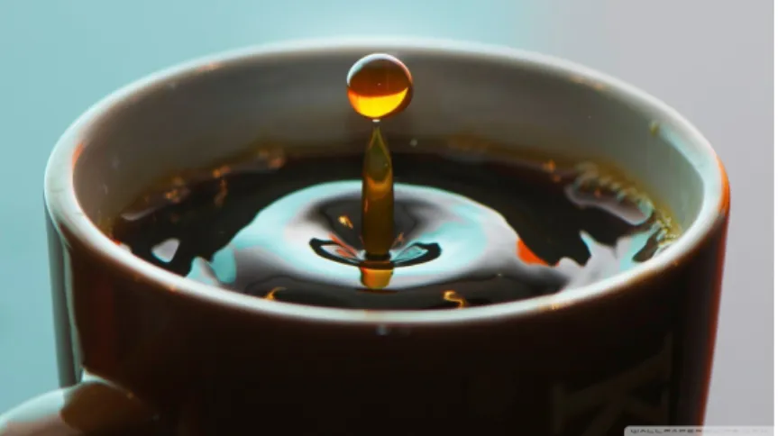
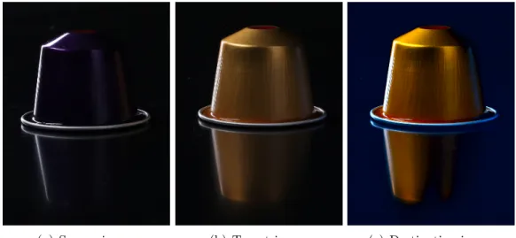
With most light sources, power variations are accompanied with changes in lighting temperature, inducing visible chroma alterations. For example, while using the classical incandescent lamps (see Figure 2.8), the lamp filament tem-perature is proportionately varying to the power alterations, so with each AC period, the light color becomes first red and gradually transforms into blue.

(44)

4. General strategy for video correction 25

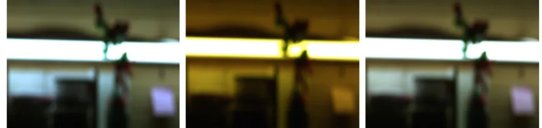
In contrast, fluorescent and LED light sources do not use a filament to produce lights, so the excitation of the chemical substances containing phosphorus, allows the perception of the emitted visible light (see an example is Figure 3.7).

Figure 2.9. Illumination / chromatic changes in a high-speed video sequence under fluorescent lighting.

4 General strategy for video correction

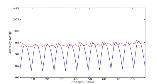
To address this periodic illumination and color variations problem, we assume that we know the acquisition frame rate and the local mains AC frequency. We therefore can estimate the period of the flickering effect. We also assume that general intensity variation integrated over few flickering periods is slow. Given this, it is easy to find the peak illumination intensity in the local period. In Figure 2.10, the acquisition frame rate is 1000 images/second and the AC mains power frequency is 100Hz. As expected, the period of the flicker is 10 frames long.

4.1 Selecting reference frames

In theory, any frame in a flicker period could serve as a reference, but we expect the reference frame to be the richest in information. However, it is easier to detect peak illumination in a period, and use the last maximum intensity frame in a period, at time tref, as a reference image. This frame may be considered as a

good choice in terms of signal-to-acquisition noise ratio.

In this goal, we computed the average of pixel intensities in each image along the sequence, so a selected reference frame in such a flicker period should be the

(45)

Figure 2.10. The blue curve shows the luminosity variation in an affected image sequence. In red we show the intensity variation in the absence of periodic flicker.

one having the highest average in this period.

As seen in Figure 2.10, changes in global illumination not related to flicker may induce low frequency variations in the luminosity of the scene.

4.2 Cross-channel correlation study

In order to check our assumption regarding the influence of periodic flicker on illumination, we acquired a sequence affected with periodic flicker due to a single source and no motion. In Figure 2.11, we plotted the cross-channel correlations between a pixel in a manually selected reference image and a subsequent frame in the same period. We observe that the vast majority of pixel colors transform linearly from the flicker-affected frame to the reference image, except at the extremal range values, due to sensor saturation effects. In the remainder, we thus assume a linear color transformation model between a reference and flicker-affected frame.

4.3 Flicker correction model

We model the color illumination transform by a 3×3 matrix Ms,t between two

(46)

4. General strategy for video correction 27

R1 G1 B1

R2

G2

B2

Figure 2.11. Cross-channel correlation between a flicker-affected frame and a reference image. respectively: Ms,t= ⎡⎢ ⎢⎢ ⎢⎢ ⎢⎢ ⎣ r₁(s, t) g₁(s, t) b₁(s, t) r₂(s, t) g₂(s, t) b₂(s, t) r₃(s, t) g₃(s, t) b₃(s, t) ⎤⎥ ⎥⎥ ⎥⎥ ⎥⎥ ⎦ . (2.12)

Using this matrix, we have

f(s′, t_ref) = Ms,tf(s, t) (2.13)

where f(s, t) ∈ R3 _{is the vector of chrominance values of pixel s at time t. This}

vector model will play a prominent role in the approaches developed in the remainder of the thesis.

(47)

(48)

Chapter 3 A short overview of

state-of-the-art techniques

In this manuscript, we are studying the problem of video color correction in the presence of complex motions. In this chapter, we first briefly describe the classical set of methods for motion estimation. We then turn to methods for dealing with illumination variations.

1 Motion estimation

The motion estimation in temporal sequences of two-dimensional images is a fundamental problem in image processing. Application areas are numerous and include image compression using motion information, robotics, meteorology with tracking cloud masses, motion tracking in medical imaging (e.g. of the heart or lungs), tracking in surveillance video systems, etc. The images are typically the projection of 3D real scenes. For this reason, we can identify three types of motion: the real motion, the apparent motion and the estimated motion. The apparent motion is often very different from the real motion and generally represents the projection of the real movement in the image plane. For example the Barber’s pole illusion, the apparent and real motion fields of a rotational motion are different.

(49)

30 Chapter 3. A short overview of state-of-the-art techniques To obtain the estimated motion, several types of methods exist. We have classified them in this chapter into four categories: feature based methods, frequency based methods, differential methods and block matching based methods.

1.1 Feature based methods

Feature based methods for object tracking is performed in two steps: the detection of features in the acquired image sequence, the matching of the detected features. The matching step should be accurate and invariant to several parameters such as the illumination variation or the occlusion of the object in order to detect efficiently the object motion.

Many approaches considering object tracking and motion detection were studied in the literature. A classification of these methods is presented byYilmaz et al. (2006). The authors distinguished 3 categories: keypoints based tracking

Serby et al. (2004), template based tracking Veenman et al.(2001); Birchfield

(1998) and shape based tracking Yilmaz et al. (2004).

Points of interest (called keypoints) in an image correspond to discontinuities of the intensity function. These can be caused, by discontinuities of the reflectance function or by depth discontinuities. They can be for example: the corners, the junctions in T or the points of strong variations of texture. A major advantage of the tracking methods based on keypoints detection is that these keypoints are in general invariant to multiple factors. Several examples of tracking based on feature points detection were proposed by Moravec (1977),Harris and Stephens

(1988) and Schmid et al.(2000).

An obvious approach for tracking an object is based on the use of a template. Indeed, if the object to be followed is of known shape (such as a car, face, etc), it is relatively simple to find the part of the image most similar to the template considered. To do this, a search is carried out exhaustively on all or part of the image. The information used can simply be intensity or color. The major disad-vantages of this method are the slowness of exhaustive search and its sensitivity to brightness variations.

(50)

1. Motion estimation 31

The representation of an object by a simple form such as a rectangle or an ellipse may be unsuitable if the target object is of a very complex shape (e.g. hand, human body, animal, tree, etc.). The representation of such an object by a corresponding shape allows to precisely take into account the shape of the object. The goal of shape based tracking methods is to estimate the shape of the objects of interest for each image of the video. This approach is related to image segmentation.

1.2 Frequency based methods

1.2.1 Fourier shift based method

This method uses the Fourier transform properties to compute the global motion between two images. It does not allow to measure the image displacement directly, but it searches in the image Fourier transform the traces of motion in order to compute the corresponding parameters. The used Fourier transform to model the problem is the continuous Fourier transform in two dimensions.

The Fourier transform preserves the rotations, and transforms a translation into a frequency shift. To calculate the translation between two images, it is sufficient to observe the phase shift between their two respective transforms.

Let F the Fourier operator, f(x, y) is an image and F(u, v) is its Fourier transformation:

F(u, v) = F[f(x, y)]. (3.1)

Let g the translation of f with a translation vector ⃗t= (δx, δy), its Fourier transform is given by

G(u, v) =F[g(x, y)]

=F[f(x + δx, y + δy)]

=e−2iπ(uδx+vδy)_F_{(u, v).} _(3.2)

(51)

32 Chapter 3. A short overview of state-of-the-art techniques A more appropriate method can be used, the phase correlation approach, as explained in the next section.

1.2.2 Phase correlation method

The phase correlation method is based on the Fourier Shift theorem (Yang et al.

(2004)) and was originally proposed for the registration of translated images. It is used for estimating the difference between two similar images or other relative translational datasets. It is commonly used in image registration and relies on a representation of data in the frequency domain, it is generally implemented by using the fast Fourier transform. The term is applied to a particular subset of cross-correlation techniques that separate the phase information from the Fourier representation space of the cross-correlogram defined below.

Definition 1. The cross-correlogram, called also cross-power spectrum is the

resulting image of cross-correlation statistics:

F(f)F(g)∗

∣ F(f) ∣∣ F(g) ∣ =e2iπ(uδx+vδy),

where ∗ indicates the complex conjugate.

In practice, we compute the two dimensional discrete Fourier transform (DFT) for both images and we can apply a Hamming window on the DFT result of both images to reduce boundary effects. A one dimensional Hamming function is being applied on all rows and columns separately.

Definition 2. The Hamming windowing, also called weighting window, is a

clas-sical technique used to focus on a section of measured signal, in order to minimize the distortions that cause a spectral leakage of the Fast Fourier Transform. The associated one-dimensional window is given by

h(t) =⎧⎪⎪⎪⎨⎪⎪⎪

⎩

0.54− 0.46 cos 2πt

T, if t∈ [0, T]

(52)

1. Motion estimation 33

The normalized cross correlation between the two transforms is then calculated. The best phase shift is the one that minimizes the cross correlation function.

Figure 3.1. Phase correlation exampleZitova and Flusser(2003): the graph on the left depicts red-red channel matching and the right one demonstrates red-blue channel matching. The peaks correpond to the matching positions.

De Castro and Morandi (1987) extended the phase correlation method to include the rotation transformation. An affine image registration is performed using phase correlation and log-polar mapping based on a log-polar coordinates system (where a point is identified by two numbers, one for the logarithm of the distance to a certain point, and one for an angle) by Wolberg and Zokai

(2000). Foroosh et al. (2002) have introduced a phase correlation extension for sub-pixel registration by means of the analytical expression of phase correlation on downsampled images.

The phase correlation technique is relatively robust because all frequencies contribute to the calculation of correlation coefficients, and it is relatively fast thanks to the fast Fourier transform, but it is practically limited to global, translation-only transforms on the whole image.

Flicker Removal and Color Correction for High Speed Videos

HAL Id: tel-01744714

https://pastel.archives-ouvertes.fr/tel-01744714

Flicker Removal and Color Correction for High Speed

Videos

Ali Kanj

To cite this version:

Docteur en Traitement du Signal et des Images

Flicker Removal and Color Correction for High

Speed Videos

Ali KANJ

Acknowledgements

Contents

List of Figures

Chapter 1

Introduction

1

Context

2

Collaboration

3

Organization of the manuscript

4

Publications

Chapter 2

Generalities on color acquisition

devices, and introduction to the

flicker removal problem

1

Color cameras

1.1

Color representation systems

1.2

Acquisition systems

1.3

Color filter array

2

High speed acquisition

2.1

Brief history

2.2

Applications

3

The flicker problem

3.1

State of the art

3.2

Flicker in high speed acquisition under artificial

light-ing

3.3

Flicker analysis

4

General strategy for video correction

4.1

Selecting reference frames

4.2

Cross-channel correlation study

4.3

Flicker correction model

Chapter 3

A short overview of

state-of-the-art techniques

1

Motion estimation

1.1

Feature based methods

1.2

Frequency based methods