HAL Id: tel-02296952
https://pastel.archives-ouvertes.fr/tel-02296952
Submitted on 25 Sep 2019HAL is a multi-disciplinary open access archive for the deposit and dissemination of sci-entific research documents, whether they are pub-lished or not. The documents may come from teaching and research institutions in France or abroad, or from public or private research centers.
L’archive ouverte pluridisciplinaire HAL, est destinée au dépôt et à la diffusion de documents scientifiques de niveau recherche, publiés ou non, émanant des établissements d’enseignement et de recherche français ou étrangers, des laboratoires publics ou privés.
Photon-pair generation in hollow-core photonic-crystal
fiber
Martin Cordier
To cite this version:
Martin Cordier. Photon-pair generation in hollow-core photonic-crystal fiber. Optics / Photonic. Université Paris Saclay (COmUE), 2019. English. �NNT : 2019SACLT024�. �tel-02296952�
Photon-pair generation in
hollow-core photonic-crystal fiber
Thèse de doctorat de l'Université Paris-Saclay
préparée à Télécom ParisTech
École doctorale n°572 Ondes et Matière (EDOM)
Spécialité de doctorat: PhysiqueThèse présentée et soutenue à Paris, le 17 mai 2019, par
Martin CORDIER
Composition du Jury : Mme. Virginia D’AURIA
Maître de conférences, Université Nice Sophia Antipolis Rapporteur
M. Nicolas TREPS
Professeur, Laboratoire Kastler Brossel Rapporteur
Mme. Catherine LEPERS
Professeur, Télécom SudParis Président du Jury
M. Michael RAYMER
Professeur, University of Oregon Examinateur
Mme. Eleni DIAMANTI
Chargée de Recherche, LIP6 Invitée
M. Fetah BENABID
Directeur de recherche, XLIM Invité
Mme. Isabelle ZAQUINE
Professeur, LTCI, Télécom ParisTech Directeur de thèse
M. Philippe DELAYE
NNT
:
2
0
1
9
S
A
CL
T0
2
4
Contents i
INTRODUCTION 7
A Spontaneous four-wave mixing for photon-pair generation 13
A1 Spontaneous Four-Wave Mixing in Optical Fiber 16
1.1 Dielectric Polarization . . . 16
1.2 Electromagnetic fields . . . 20
1.3 Deriving the Hamiltonian . . . 22
A2 Joint Spectral/Temporal Amplitude 31 2.1 Joint Spectral Amplitude . . . 31
2.2 Schmidt decomposition . . . 37
2.3 Group velocity matching . . . 43
2.4 Joint Temporal Amplitude and Phase Correlation . . . 46
2.5 The spectral density map . . . 49
A3 Avoiding Raman scattering 52 3.1 Description of Raman scattering . . . 52
3.2 Possible Solutions . . . 56
B Liquid-filled PBG Fiber: Toward Telecom Raman-free photon pair source 59 B1 Design of the Liquid-filled PBG-HCPCF 62 1.1 Guidance mechanism of Photonic Bandgap Fiber (PBG) . . . 62
1.2 Finding the right Fiber/Liquid combination . . . 65
1.3 Experimental Linear Characterization . . . 71
1.4 Experimental Nonlinear Characterization . . . 75
Contents
B2 Toward Raman-free four-wave mixing 82
2.1 Computed Spectral Density Map . . . 82
2.2 Experimental setup and filtering . . . 86
C Raman-free photon-pair generation and spectral correlations engineering in Gas-filled IC fiber 93 C1 Spectral correlation engineering and fiber design 96 1.1 Introduction to spectral-correlation engineering . . . 96
1.2 Comparison between PBG and IC . . . 100
1.3 IC fiber analytical model . . . 108
1.4 Multiband FWM - Spectral correlation engineering . . . 114
1.5 Design of the gas-filled source . . . 116
1.6 Chosen design . . . 120
C2 Joint Spectral Intensity tomography 124 2.1 JSA characterization techniques . . . 124
2.2 Experimental tomography setup . . . 126
2.3 Experimental JSI (Phase Matching Engineering) . . . 128
2.4 Pulse shaping . . . 132
2.5 Experimental JSI (Pump spectrum Engineering) . . . 135
C3 Raman-free photon-pair generation 144 3.1 Experimental setup . . . 144
3.2 Count measurements . . . 146
3.3 Coincidence measurements . . . 150
3.4 Spectral tunability through gas-pressure . . . 158
CONCLUSION & PERSPECTIVES 159 Appendix 166 I SDM calculation . . . 167
II Spectral phase correlation . . . 168
III Articles . . . 169
Comme chacun le sait, la recherche est un travail au long cours avec des issues souvent incertaines. C’est ce qui la rend à la fois très difficile et incroyablement satisfaisante. J’ai passé de nombreuses heures dans l’obscurité la plus totale, fixant un écran d’ordinateur rougi pour les verres colorés des lunettes de protections laser, à « chercher des paires de photons ». Et pourtant, derrière cette scène un peu absurde du quotidien d’un physicien expérimentaliste, il y avait là, l’aboutissement de ma thèse. En effet, un nouveau record été battu sous mes yeux, preuve ultime de la démonstration d’une idée que nous avions eu deux ans auparavant. En prenant du recul sur ces trois ans et demi de thèse, ce qui me marque le plus, c’est la confiance sans faille qui m’a été accordée. Dans ces quelques lignes, je voudrais remercier toutes les personnes qui l’ont exprimée.
En premier lieu, je voudrais remercier Isabelle Zaquine pour son encadrement de tous les instants lors de cette thèse et du stage qui a précédé. C’est grâce à son dévouement et sa combativité que j’ai pu obtenir une bourse de thèse. Tout en m’offrant une grande liberté d’action sur l’orientation que je voulais donner à ces recherches, sa présence au quotidien a donné un cadre idéal à ce travail de thèse. Sa grande écoute et ses conseils avisés m’ont permis de prendre du recul et ont été une grande source d’encouragement.
Je souhaiterais également remercier Philippe Delaye qui a co-encadré cette thèse. Je ne pourrais compter le nombre de fois où sa fine connaissance d’optique non linéaire est venue éclairer mes interrogations. Tant j’ai pu y apprendre, ces longues discussions ont été l’un des pivots de ma thèse et une grande source d’enrichissement personnel. J’ai eu également la grande chance de passer du temps dans son équipe à l’Institut d’Optique et de travailler avec mon ami Thibault Harlé qui effectuait une thèse en parallèle de la mienne.
Un grand merci également à Fetah Benabid qui m’a accueilli dans son équipe à Limoges pendant plus d’un an et qui a tout mis en œuvre pour que cette collaboration soit fructueuse. L’enthousiasme et la passion qu’il avait pour mon travail m’ont grandement inspiré et encour-agé. Cette collaboration a aussi été rendue possible grâce à Frédéric Gérome et Benoit Debord qui m’ont régulièrement prodigué de précieux conseils sur les fibres. Bien sûr ces journées à Limoges n’auraient pas été les mêmes sans la Dream Team du GPPMM: Foued, Matthieu,
Contents
Martin, David, P’tit Fred, Aymeric, Jonas, Mustafa, Thomas, Maxime, Ali ainsi que celle de GLO : Alex, Ando, Grand Ben’. C’était un plaisir quotidien de travailler avec vous tous!
Merci à tous mes collègues de Télécom, Eleni Diamanti pour ses précieux conseils, sa bonne humeur et son humour ! Je remercie Adeline Orieux à qui ce travail doit beaucoup tant elle m’a aidé. Merci à Julien et Mathieu pour la bonne ambiance au labo et d’avoir partagé leur passion pour la musique et à Eliseu pour toutes les passionnantes discussions philosophiques que nous avons eues. Merci aux permanents du groupe Romain Alléaume, Filippo Miatto et à Renaud Gabet pour avoir pris le temps de m’introduire à l’OLCI. Merci aussi à Ravi pour ses nombreux conseils !
Mes remerciements vont également à mes deux rapporteurs, Virginia D’Auria et Nicolas Treps et aux examinateurs Catherine Lepers et Michael Raymer d’avoir porté intérêt et con-sidérations à mes travaux. Merci à l’ensemble du jury pour leurs remarques, questions et échanges lors de la soutenance.
Je souhaiterais aussi adresser mes remerciements aux professeurs qui ont éveillé en moi une passion pour la physique. En particulier, Arnaud Devos, dont les cours de physique quantique ont été une vraie claque et dont le stage que j’ai effectué avec lui a été une expéri-ence passionnante, fondatrice de mon parcours de recherche. Un grand merci également à Bruno Grandidier, Christophe Delerue et Agnès Maitre qui m’ont permis de faire un master de physique fondamentale en parallèle de mes études d’ingénieur.
Merci à mes parents et à mes deux sœurs qui m’ont toujours soutenu et encouragé à suivre ma propre voie. Enfin, un immense merci, Daga, pour le bonheur et l’amour que tu apportes à ma vie.
Abstract [En]
The thesis reports on the design of photon-pair sources based on fluid-filled hollow-core photonic crystal fiber (FF-HCPCF). It combines two important properties: (1) Raman-free gen-eration thanks to the use of a fluid and to a minute overlap with silica within the hollow-core ; (2) a high versatility in the phase-matching conditions thanks to the fiber microstructuration and choice of fluid.
In order to design a versatile Raman-free photon-pair source, we explored two approaches that entails different waveguiding designs and fluid-filling processes.
On the one hand, we investigate the use of a liquid-filled photonic bandgap HCPCF. We demonstrate that there exists Raman-free spectral range at telecom wavelength compatible with photon-pair generation. On the other hand, we develop, to our knowledge, the first photon-pair source in a gas-filled inhibited-coupling HCPCF which goes along with the first demonstation of Raman-free photon-pair generation in a fiber medium. The source was designed to operate at convenient wavelengths for heralded single photon source; the idler wavelength lies in the telecom wavelength range, while the signal wavelength is in the range of atomic transitions and Silicon single photon detectors. Moreover, we demonstrate experimentally a passive and active control over the generated photon spectral properties. In particular, spectral correlations can be tailored, allowing spectrally entangled and factorable states to be obtained within the same device. More specifically, a gallery of different joint spectral intensity, including exotic shape, is measured by tuning various parameters: gas pressure, pump spectral width, spectral chirp and pump spectral envelope. Furthermore, this photon-pair state is generated over a tunable frequency-range that spans well over tens of THz.
Thus, the present thesis presents both theoretical and experimental results demonstrating the capability of hollow-core photonic crystal fibers to generate Raman-free photon-pair with controllable spectral properties.
Contents
Abstract [Fr]
Cette thèse porte sur la conception de fibres à cristaux photoniques à coeur creux remplies de fluide (FF-HCPCF) pour la génération de paires de photons. Ces sources combinent deux propriétés importantes: (1) l’absence de bruit Raman grâce à l’utilisation de fluides et d’un recouvrement optique très limité avec la silice au sein de la fibre; (2) une grande polyvalence dans les conditions d’accord de phase grâce à la microstructuration de la fibre et au choix du fluide.
Dans l’objectif de concevoir une source de paires de photons sans bruit Raman, nous avons exploré deux approches impliquant à la fois des mécanismes de guidages et des types de fluides de remplissages différents.
D’une part, nous avons étudié l’utilisation de fibres à coeur creux à bande interdite photonique, remplies de liquide. Nous démontrons qu’il existe une gamme spectrale aux longueurs d’ondes télécom sans bruit Raman compatible avec la génération de paires de photons. D’autre part, nous avons également développé la première source de photons dans une fibre HCPCF à couplage inhibé remplie de gaz qui a permis la première démonstration de génération de paires de photon sans Raman dans un milieu fibré. La conception de la fibre a été choisie pour fonctionner à des longueurs d’ondes utiles aux sources de photons annoncées ; la longueur d’onde idler se situe dans le domaine télécom, tandis que la longueur d’onde signal est dans la gamme visible des détecteurs de photon unique silicium. De plus, nous démon-trons expérimentalement un contrôle actif et passif des propriétés spectrales des photons générés. En particulier, les corrélations spectrales peuvent être modifiées afin d’obtenir un état spectrallement factorisable ou corrélé au sein du même dispositif. Plus précisément, une variété d’intensités spectrales jointes (JSI) de formes différentes, dont certaines exotiques, ont été mesurées en faisant varier différents paramètres : la pression du gaz, la largeur spectrale de la pompe, le chirp ainsi que l’enveloppe spectrale de la pompe. Enfin, la paire de photons est générée sur une plage de fréquence accordable qui s’étend sur des dizaines de THz.
Ainsi, la présente thèse expose des résultats théoriques et expérimentaux démontrant la génération de paires de photons sans diffusion Raman et avec des propriétés spectrales con-trôlables.
AOPDF: acousto-optic programmable dispersive filter Ar: argon
BS: beam splitter
BSMF: birefringent single mode fiber CAR: coincidences to accidental ratio CW: continuous wave
DC: dark count DM: dichroic mirror
DSF: dispersion shifted fiber DUT: device under test
FDFD: finite difference frequency domain FT: Fourier transformation
FWHM: full width at half maximum FWM: four-wave mixing
GF: gas-filled
GVD: group-velocity dispersion GVM: group-velocity matching
HCPCF: hollow-core photonic crystal fiber HWP: half-wave plate
IC: inhibited-coupling
JSA/JSI: joint spectral amplitude/intensity JTA/JTI: joint temporal amplitude/intensity LF: liquid-filled
OLCI: optical low coherence interferometry OSA: optical spectrum analyser
PBG: photonic bandgap PBS: polarising beam splitter PCF: photonic-crystal fiber RS: Raman-scattering
Contents
SDM: spectral density map
SEM:scanning electron microscope SET: stimulated emission tomography Si: silica
SLM: spatial light modulator SM: surface mode
SMF: single mode fiber SNR: signal to noise ratio SPD: single photon detector
S-SPD: superconducting single photon detector SPDC: spontaneous parametric down conversion TIR: total internal reflection
TM: temporal mode
WDM/CWDM/DWDM: wavelength division multiplexer / coarse WDM / dense WDM Xe: xenon
Based on the laws of quantum mechanics, quantum information science has the potential for significantly improving our modern technologies. More specifically, it paves the way to an im-provement in terms of computational power (quantum computing) and communication secu-rity (quantum communication). The conjoint ability to encode, manipulate and communicate quantum mechanical objects are the sine qua non condition on the roadmap toward the devel-opment of quantum technologies. In this fast-growing field, the capability to distribute quan-tum bits (qubits) to remote locations is highly desirable and photons provide the ideal flying
qubits - the quantum information carrier for large distance communication [1].
In this context, non-classical states of light, encompassing single photons, entangled photon-pair states and squeezed states are one of the central element of quantum information. The development of non-classical light source at telecom wavelength is the focus of this work.
Photon pair sources
One of the most widespread sources of non-classical states of light are photon-pair sources, also called heralded single photon sources. The photon generation process is based on nonlin-ear effects allowing to probabilistically annihilate photons from an intense pump and simul-taneously generate two photons at different frequencies (called signal and idler). In general, these effects are either spontaneous parametric down conversion (SPDC) or four-wave mixing (FWM) depending on whether the medium has aχ(2)orχ(3)nonlinearity.
Fig. 1: Schematic describing a photon-pair source. The filled dots corresponds to photons whereas
the empty dots corresponds to a non-generation (probabilistic process).
been historically the workhorse for photon pair generation due to the relative ease in terms of experimental setup, their cost and their availability. Today, KDP (potassium dideuterium phosphate), BBO (beta barium borate), LiNbO3 (lithium niobate) and LiIO3 (lithium iodate) are typically chosen for the strength of theirχ(2)nonlinearity, which is directly linked to the photon pair generation efficiency. As far as the use of cristals is concerned, the pioneering work of Kwiat et al. [2] should be mentioned.
Although generally less nonlinear, χ(3) media, and in particular waveguides and optical fibers have gained much attention in the recent years, offering new prospects in terms of scal-ability and integrscal-ability. For instance, more than 550 photonic components have been recently integrated on a single silicon chip, including 16 identical four-wave mixing photon-pair sources [3]. Alternatively, fiber-based photon-pair sources have many advantages; they are easily man-ufacturable, cost effective, robust, alignment-free and compatible with fiber optical network since the photon pairs are directly emitted in the fundamental transverse mode of a fiber.
Fiber architectures
As far as fibers are concerned, photon-pairs have been produced in many different ar-chitectures encompassing single-mode fiber (SMF) [4, 5], dispersion-shifted fiber (DSF) [6, 7, 8, 9], birefringent single-mode fiber (BSMF) [10, 11] and photonic crystal fiber (PCF) [12, 13, 14, 15, 16, 17, 18]. However, the performances of these photon-pair sources are most often plagued by a concomitant nonlinear effect, Raman-scattering (RS). Indeed, in addition to the four-wave mixing which leads to photon-pair generation, an interaction between the pump and phonons in the medium results in the generation of scattered photons. Due to the amorphous nature of silica (i.e. the fiber core material), the Raman gain is broadband [19], thus generating a large amount of scattered photons around the pump frequency. In fact, whatever the photon-pair frequencies, some Raman-scattered photons will also be generated at the same frequencies, that cannot be filtered. For this reason, Raman-scattering degrades the achievable signal to noise ratio. Raman-scattering can be reduced by cooling down the fiber to cryogenic temperature with nitrogen (T = 77 K) [4, 8, 9] or even helium (T = 4 K) [7], however it cannot be completely suppressed and it adds a layer of experimental difficulty making it much less practical for applications and limited in terms of integration.
An ideal solution consists in changing the propagation medium (silica) to one without a broadband Raman gain. Unfortunately, any other glass (chalcogenide, tellurite, fluoride, etc.) does not solve this issue since all amorphous materials exhibit broad Raman gain spectra [20, 21]. In contrast, there is a particular kind of fiber which allows to guide light with a negligible overlap with the glass: hollow-core photonic crystal fiber (HCPCF).
Hollow-core photonic crystal fiber
Since their first developments 20 years ago, hollow-core photonic crystal fibers (also called hollow-core fiber) have attracted huge interest by virtue of their optical properties that are non-existent in conventional fibers. The empty core can be filled (with a gas, liquid, cold atoms, biological compunds, etc.) allowing to microconfine light and matter over lengths up to kilometers. For these reason, HCPCF have become a remarkably useful tool in many fields such as: atom optics, nonlinear optics, metrology as well as high optical field physics and plasma (see [22, 23] for reviews). More specifically, HCPCF can be subdivided into two families denominated by their guidance mechanisms, namely, photonic bandgap (PBG) and inhibited
coupling (IC) HCPCF. As we will detail later on, they exhibit very different optical properties
(e.g. transmission bandwidth, loss, dispersion, etc) and geometrical designs (see Fig. 3).
Our strategy is to fill HCPCFs with a fluid with either discrete Raman lines (liquid) or non-existent (noble gas) in order to avoid the overlap between Raman-scattered photons and photon-pairs. By eliminating the Raman-scattering issue, the principal motivation behind this work is to design photon pair sources with a high signal to noise ratio while keeping a fiber based architecture and its advantages (room temperature, alignment-free, robustness, etc.). In the past, HCPCFs have already demonstrated the ability to explore Raman-free nonlinear op-tics [24] but only few works have investigated quantum information applications. Barbier et al. [25] use a Liquid-filled PBG-HCPCF to obtain what is to our knowledge the first and, apart from the work presented in this manuscript, only demonstration of photon pairs in such media. In [25], the authors have shown that Raman-scattering is reduced by three orders of magnitude compared to a silica-core fiber. In another regime, Finger et al. [26, 27] report a Raman-free squeezed-vacuum bright twin-beam source based on IC-HCPCF filled with a noble gas (argon).
Fig. 2: Comparison between Raman scattering in silica core fibers (SMF, DSF, BSMF, PCF) and in a
hollow-core fiber (HCPCF) filled with a noble gas. In silica, the Raman process generates noise at lower (Stokes) and higher (Anti-Stokes) frequencies than the pump whereas in a monoatomic noble gas, no Raman-scattering occur because of the absence of molecules. Relative intensities are arbitrary.
Objectives of the thesis
The main objective of the thesis was to design photon-pair sources based on hollow-core fibers.
Initially, I have undertaken to extend the work of Barbier et al. in order to have a hollow-core photon-pair source at telecom wavelengths (rather than in the near infrared). Starting from scratch, at the beginning of the thesis the first step has been to find a good architecture of fiber and liquid. In this regard, I have developed simulation tools to infer the optical properties of these fibers depending on their geometrical design and of the filling medium and I have per-formed experimental linear and nonlinear characterizations. Once the fiber architecture was found, I built an experimental setup to characterize its performance in the photon-pair regime.
In parallel to this work, I have also investigated how to adapt hollow-core fiber designs in order to explore spectral correlation engineering. A control of the photon-pairs spectral prop-erties is of utmost importance in most quantum information applications. I showed that it can be realized by tailoring the dispersion properties of the fiber using a control of the fiber mi-costructure. As a result from this study, I discovered how a specific type of hollow-core fiber (the inhibited-coupling fiber) exhibits all the requirements in that regard. More specifically, I have identified that the multiband dispersion profile of such fibers can be used to tailor the phase-matching conditions and to control the degree of time-frequency entanglement. I took the opportunity of an on-going collaboration with the GPPM group of XLIM, which detains state of the art hollow-core fabrication facility, to test this hypothesis experimentally. I identified a new fiber design, here based on a gas-filling (xenon) and demonstrate the first photon-pair generation in such a medium. Emphasis was placed onto designing the photon-pair source for heralded-single photon source. Signal and idler are created at benchmark wavelengths (tele-com and visible range) and the photon-pair spectral properties are tailored (into factorable state). Moreover, as I will detail, the gas-filling allows reaching unprecedented signal to noise ratio compared to other fiber architectures.
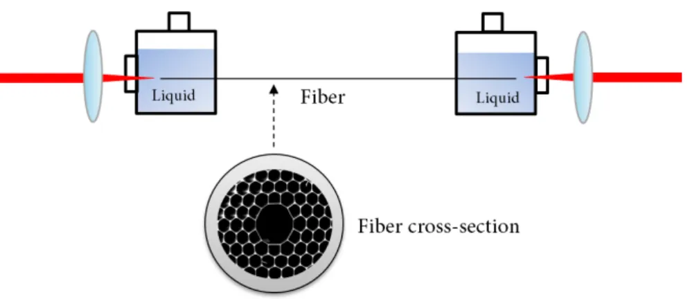
Fig. 3: Cross section of a. the liquid-filled photonic bandgap HCPCF used in Part B b. the gas-filled
inhibited coupling HCPCF used in Part C. The white areas correspond to silica and the black areas are filled with either the liquid or gas. c. Photo showing the sealed gas cells and fiber from Part C.
Outline of the thesis
The manuscript is composed of three parts.
- Part A provides the theoretical framework. The first chapter A1 describes FWM photon-pair generation in an optical fiber. The second chapter A2 introduces useful tools to de-scribe the spectral properties of the photon-pair: the Joint Spectral Amplitude (JSA) and the Schmidt decomposition. In particular, the notion of spectral correlation/spectral en-tanglement and its consequences are discussed. Finally, the Raman scattering process and its characteristics depending of the medium (diatomic, silica, liquid, gas, etc.) are described in chapter A3.
- Part B presents a Liquid-filled PBG-HCPCF based on a commercial HCPCF. While the first demonstration of photon-pair in this medium was in the infrared wavelength range [25], herein we design a source toward the generation of photon-pairs at telecom wavelength. In the first chapter, several combinations of liquids and fibers are investigated through experimental characterizations and simulations. The second chapter describes how the Raman-scattering noise can be avoided in such liquid-filled fibers and our experimental setup.
- Part C describes the Gas-filled IC-HCPCF. We demonstrate for the first time to our knowl-edge a photon-pair source in such media and its Raman-free property. The first chapter introduces the concept of spectral correlations manipulation and why it is important in view of quantum information applications. Moreover, after describing the inhibited coupling guidance mechanism, we show theoretically how the IC fibers design offer a huge versatility in tailoring the photon-pair spectral properties (including spectral cor-relations). We demonstrate experimentally this versatility in the second chapter by per-forming a spectral tomography of the generated biphoton state. Finally, the third chapter presents the characterisation of the source in the photon-pair regime.
Spontaneous four-wave mixing for
photon-pair generation
following of the manuscript. In the first chapter, a model is given to describe spontaneous four-wave mixing nonlinear process and to derive the photon-pair state as a function of both medium and pump parameters. The second chapter introduces key-concepts: (i) the joint-spectral ampli-tude function and (ii) the spectral density map which describe the photon-pair time-frequency properties. The last chapter describes another nonlinear effect of importance in this manuscript, Raman-Scattering, and why it is generally detrimental for photon-pair generation.
Chapter A1: Spontaneous Four-Wave Mixing in Optical Fiber Chapter A2: Joint Spectral/Temporal Amplitude
Chapter A1
Spontaneous Four-Wave Mixing in
Optical Fiber
1.1 Dielectric Polarization . . . 16 1.2 Electromagnetic fields . . . 20 1.3 Deriving the Hamiltonian . . . 22
In this chapter, we derive a semi-quantum description to detail the spontaneous four-wave mixing nonlinear effect. In this approach, the electromagnetic fields describing individual pho-tons are quantized whereas the pump and the medium are considered classical. Starting from the Schrödinger equation, the nonlinear Hamiltonian and the photon pair wavefunction are derived.
The development is inspired by the thesis manuscripts of Warren Paul Grice [28] and Mar-gaux Barbier [29] who both derived a semi-classical and a quantum model for describing the generation of photon pair through four-wave mixing.
1.1 Dielectric Polarization
a) Linear regimeIn the linear regime, the propagation of an electromagnetic wave in matter is influenced by the dielectric polarization induced by the electric field of the wave. The dielectric susceptibilityχ(1) relates the dielectric polarization to the electric field [30]:
ˆ Pi(r, t ) = ²0 X j χ(1) i j(ω)ˆEj(r, t ) (A1.1)
where²0is the vacuum permittivity,χ(1)is a rank 2 tensor, expressed in the form of a 3x3 matrix, and the indices i and j take the values of the Cartesian coordinates (x,y,z).
b) Nonlinear regime
In a regime of strong electromagnetic field, the dielectric response to the electromagnetic field is no longer linear and Eq. (A1.1) is no longer valid. Then, the polarization of a transparent media is given by [30]: ˆ Pi= ²0 X j χ(1) i jEˆj | {z } linear + ²0 X j X k χ(2) i j kEˆjEˆk+ ²0 X j X k X l χ(3) i j klEˆjEˆkEˆl+ ... | {z } non linear (A1.2)
where each [χ(k)] is a real k+1 rank tensor composed of (k + 1)k+1components such thatχ(1)i j = ei.[χ(1)]ej,χ(2)i j k= ei.[χ(2)]ejekandχ(3)i j kl= ei.[χ(3)]ejekel, with eiis the unit vector of axis i.
In the following, we will consider only isotropic media (invariance along three spatial di-rections). In that case the dielectric polarization and the electric field are parallel, such that the equation simplifies to:
ˆ
P(r, t ) = ²0χ(1)E(r, t ) + ²ˆ 0χ(2)E(r, t ) ˆˆ E(r, t ) + ²0χ(3)E(r, t ) ˆˆ E(r, t ) ˆE(r, t ) + ... (A1.3) We define:
ˆ
PL= ²0χ(1)E(r, t )ˆ (A1.4)
ˆ
PNL= ²0χ(2)E(r, t ) ˆˆ E(r, t ) + ²0χ(3)E(r, t ) ˆˆ E(r, t ) ˆE(r, t ) + ... (A1.5) The dielectric polarization is an electronic response from the medium. Hence it is expected that the nonlinear terms become non-negligible when the amplitude of the applied field is of the order of the characteristic atomic electric field strength Eat = e/a20, where e is the charge
of the electron and a0= ħ2/me2the Bohr radius [30]. Sinceχ(1)is of the order of unity, we can expect thatχ(2)is of the order of 1/Eat and thusχ(k)≈ χ(k−1)/Eat = 1/Ek−1at . Since the
suscep-tibilities quickly decrease for an increasing k order, only nonlinear effects of the second order χ(2)and third orderχ(3) susceptibilities are generally accessible with a standard laser. Hence, the higher order terms are neglected.
Let us illustrate the role of the nonlinear dielectric polarization with examples. First, we consider the case where medium is pumped by an electromagnetic field consisting of a plane wave E(t ) = ²1e−i ω1t+c.c.. The term ˆPLis the linear response of the medium. It consists of part of the electromagnetic field oscillating at the same frequencyω1. The nonlinear term ˆPNL con-tains components of the form E2and E3and therefore bears terms oscillating as twice the fre-quency (second harmonic) or three times the frefre-quency and more. The situation becomes even
1.1. Dielectric Polarization
more diverse when considering an electromagnetic field in a superposition of fields with dif-ferent central frequencies. Table A1.1 sums up all the possible difdif-ferent frequency components that can arise from a nonlinear interaction when considering a monochromatic field (first row) and a field which is a sum of two plane waves (second row). Note that the number of frequency components increases rapidly with the number of input wavelengths.
Tab. A1.1: Frequency components of the dielectric polarization induced by a plane wave. SHG: second harmonic generation, OR: optical rectification, SPM: self-phase modulation, THG: third harmonic generation, SFG: sum frequency generation, DFG: difference frequency generation
Input Field χ(1) χ(2) χ(3) E(t ) = ²1e−i ω1t ω1 2ω1(SHG) 3ω1(THG) + c.c. 0 (OR) ω1(SPM) ω1 2ω1(SHG) 3ω1(THG) ω2 2ω2(SHG) 3ω2(THG) E(t ) = ²1e−i ω1t ω1+ ω2(SFG) 2ω1+ ω2 +²2e−i ω2t+ c.c. ω1− ω2(DFG) 2ω1− ω2 0 (OR) ω1+ 2ω2 ω1− 2ω2 c) Derivation
In practice, nonlinear media often exhibit symmetries such that many components of the non-linear susceptibility tensor vanish. In the case of centrosymmetry (invariance under inversion through the origin) for instance, it can be easily shown [30] that all the even nonlinear suscep-tibilities vanish (χ(2)= 0, χ(4)= 0, etc.).
Optical fibers, whether composed of a silica core or of a hollow-core filled with a liquid or gas are centrosymmetric. Thus, the smallest nonlinear susceptibility order we consider is the third order. Discarding higher order odd terms, the dielectric polarization becomes:
ˆ
PNL(r, t ) = ²0χ(3)E(r, t ) ˆˆ E(r, t ) ˆE(r, t ) (A1.6) Let us assume that the electromagnetic field E is composed of four distinctive fields designated as pump1, pump2, signal and idler oscillating atωp1,ωp2,ωsandωi. Since we are considering
a fiber media, it is justified to restrict ourselves to electromagnetic fields propagating in the z direction, in the fundamental transverse mode of the fiber. We also consider that all four fields share the same linear polarization along e which greatly simplifies the notations.
ˆ
All the fields may be expressed in terms of their positive and negative frequency parts: ˆ
Ek(z, t ) = ˆE(+)k (z, t ) + ˆE(−)k (z, t ) (A1.8)
Distributing the different terms of the product, the nonlinear dielectric polarization is com-posed of:
ˆ
PNL(z, t ) = ²0χ(3)³Eˆp1(z, t )3+ ˆEp2(z, t )3+ ˆEs(z, t )3+ ˆEi(z, t )3 (A1.9)
+ 3 ˆEp1(z, t )2Eˆp2(z, t ) + 3 ˆEp1(z, t )2Es(z, t ) + 3 ˆEp1(z, t )2Eˆi(z, t )
+ 3 ˆEp2(z, t )2Eˆp1(z, t ) + 3 ˆEp2(z, t )2Eˆs(z, t ) + 3 ˆEp2(z, t )2Eˆi(z, t )
+ 3 ˆEs(z, t )2Eˆp1(z, t ) + 3 ˆEs(z, t )2Eˆi(z, t ) + 3 ˆEs(z, t )2Eˆp2(z, t )
+ 3 ˆEi(z, t )2Eˆp1(z, t ) + 3 ˆEi(z, t )2Eˆs(z, t ) + 3 ˆEi(z, t )2Eˆp2(z, t )
+ 6 ˆEp1(z, t ) ˆEs(z, t ) ˆEi(z, t ) + 6 ˆEp2(z, t ) ˆEs(z, t ) ˆEi(z, t )
+ 6 ˆEp1(z, t ) ˆEp2(z, t ) ˆEs(z, t ) + 6 ˆEp1(z, t ) ˆEp2(z, t ) ˆEi(z, t )
´
Such general expression describes the collection of allχ(3)nonlinear effects which comprises the possible third harmonic generation, four-wave mixing, self phase modulation and cross phase modulation. In total, it contains 40 different frequency components around:
h 3ωp1, 3ωp2, 3ωs, 3ωi,ωp,ωs,ωi, 2ωp1± ωp2, 2ωp1± ωs, 2ωp1± ωi 2ωp2± ωp1, 2ωp2± ωs, 2ωp2± ωi, 2ωs± ωp1, 2ωs± ωp2, 2ωs± ωi 2ωi± ωp1, 2ωi± ωp2, 2ωi± ωs,ωp1± ωp2± ωs,ωp1± ωp2± ωi ωp1± ωs± ωi,ωp2± ωs± ωi i
Typically, no more than one of these frequency components will be generated in the medium. In addition to energy conservation, the process must fulfil a certain phase-matching condition which ensures that the waves radiated by the nonlinear polarization in the whole crystal inter-feres constructively through the propagation. In the following, only the parametric four-wave mixing terms fulfillingωp1+ ωp2− ωs− ωi = 0 are kept. All other effects are considered not
phase-matched and are therefore discarded. We are left with four terms: ˆ PNL(z, t ) = ²0χ(3) ³ 6 ˆE(+)p1(z, t ) ˆE(−)s (z, t ) ˆE(−)i (z, t ) + 6 ˆE(+)p2(z, t ) ˆE(−)s (z, t ) ˆE(−)i (z, t ) (A1.10) + 6 ˆE(+)p1(z, t ) ˆE(+)p2(z, t ) ˆE(−)s (z, t ) + 6 ˆE(+)p1(z, t ) ˆE(+)p2(z, t ) ˆE(−)i (z, t ) ´ + h.c
In fact, the different terms of Eq. (A1.10) lead to the same nonlinear effect of the form χ(3)Eˆ(+)
p1Eˆ (+) p2Eˆ
(−)
s Eˆ(−)i as we will see later when deriving the Hamiltonian (see section A.1.3). This
degeneracy is known as the Kleinman’s symmetry1which is valid whenever we consider fre-quencies far from resonances of the medium.
1.2. Electromagnetic fields
Fig. A1.1: Illustration of different possibleχ(3)nonlinear interactions leading to a dielectric polariza-tion at some given new frequency. The black arrows are the interacting input fields and the nonlinear polarization frequency is represented by a gray arrow.
1.2 Electromagnetic fields
a) Signal and idler fields
Assuming that the spectrum of each mode in the fiber is concentrated around a central fre-quencyωj, the quantized electromagnetic field is given by [28]:
ˆ E(z, t ) =X kj i s ħωj 2VQ²0n2(ωj) ˆ akje i (β(ωj)z−ωjt )+ h.c (A1.11)
where VQis the quantization volume, n(ωj) is the frequency dependent index of refraction and
ˆ
akj is the annihilation operator for the mode characterized by wave vector k = β(ωj)ez. Note that, we use the notation convention of the fiber optic community where the z-component of the wavevector kz is commonly denominated asβ.
It is convenient to convert the finite summations into integrals [31, 29]: X kj → Z LQ dkj 2π → Z LQβ1(ωj) dωj 2π (A1.12) ˆ akj → ˆ a(kj) pLQ → a(ˆ ωj) qβ1(ωj)LQ (A1.13)
Such that: ˆ E(z, t ) = Aj Z dωja(ˆ ωj)ei (β(ωj)z−ωjt )+ h.c (A1.14) where Aj =2iπ r ħωjβ1(ωj) 2Aeff²0n2(ωj), withβ1= dk dω and Aeff= VQ
LQ taken as the fiber transverse effective area with LQthe quantization length.
We use the slowly varying envelope approximation, i.e. the bandwidth of the considered electric field is small compared to its central frequency. This allows us to extract the Aj from
the integral. Such approximation is justified since we only consider narrow spectrum electric fields.
The creation and annihilation operators satisfy the usual commutation relations:
[ ˆa(ω), ˆa†(ω0)] = δ(ω − ω0) (A1.15a)
[ ˆa(ω), ˆa(ω0)] = 0 (A1.15b)
In the end, signal and idler field are described by: ˆ Es(z, t ) = As Z dωsa(ˆωs)ei [β(ωs)z−ωst ]+ h.c (A1.16a) ˆ Ei(z, t ) = Ai Z dωia(ˆ ωi)ei [β(ωi)z−ωit ]+ h.c (A1.16b) b) Pump fields
The pump fields are much stronger than the signal and idler fields and are assumed to be un-depleted as they propagate through the fiber. Accordingly, the pump fields may be replaced by classical fields of the form:
ˆ
Ep1(z, t ) ≈ Ep1(z, t ) = Ep1(t )eiβ(ωp1)z+ c.c (A1.17a)
ˆ
Ep2(z, t ) ≈ Ep2(z, t ) = Ep2(t )eiβ(ωp2)z+ c.c (A1.17b)
And their Fourier decompositions are given by: Ep1(z, t ) = Z +∞ −∞ dωp1 ˜ Ep1(ωp1)ei (β(ωp1)z−ωp1t ) (A1.18a) Ep2(z, t ) = Z +∞ −∞ dωp2E˜p2(ωp2)ei (β(ωp2)z−ωp2t ) (A1.18b)
Where ˜Epis the Fourier transform of the temporal envelope of the field. Note that, no
1.3. Deriving the Hamiltonian
Having defined the non-linear polarisation and the fields, we can derive the non-linear Hamiltonian to describe the four-wave mixing process.
1.3 Deriving the Hamiltonian
In quantum physics, there exist distinct representations among which the three most com-monly used: (i) the Schrödinger, (ii) the Heisenberg and (iii) the Interaction pictures (the later being also called Dirac picture). While mathematically equivalent, they differ from each other in the role that the wavefunction and the operators bear. In the Schrödinger picture, the wave-function is time-dependent as opposed to operators which remain fully time-independent. The Heisenberg picture it is the exact opposite. Finally, the Interaction picture lies halfway, with both the wavefunction and operators bearing a certain time-dependence. When an in-tense pulse of light propagates through the medium, the Hamiltonian describing the system can be decomposed into a linear part ˆHL and a non-linear part ˆHNL, the latter being consid-ered a perturbation ( ˆH = ˆHL+ ˆHNL).
Schrödinger Heisenberg Interaction
i ħd dt ¯ ¯ψS(t )® = ˆH¯¯ψS(t )® d dt ¯ ¯ψH(t )® = 0 i ħ d dt ¯ ¯ψI(t )® = ˆHNL¯¯ψI(t )® d ˆOS dt = 0 i ħ d ˆOH dt = h ˆ OH; ˆH i d ˆOI dt = h ˆ OI; ˆHL i
In our case, we adopt the Interaction picture which has the advantage of allowing to focus on the nonlinear contribution only. Indeed, the state is determined by solving a Schrödinger equation of the form:
i ħd dt ¯ ¯ψ(t)® = ˆHNL(t ) ¯ ¯ψ(t)® (A1.19)
From which we deduce:
¯
¯ψ(t + dt)® = e− i
hHˆNL(t ) dt¯
¯ψ(t)® (A1.20)
Before the pump pulse interacts with the medium (t < 0), the signal and idler are void of any photon. The initial state at t = t0is then |0s, 0i〉 such that we can write:
¯ ¯ψ(t0)® = e− i ħ Rt 0 t0HˆNL(t ) dt |0s, 0i〉 (A1.21)
the exponential [32]: ¯ ¯ψ(t0)® ≈ h 1+−i ħ Z t0 t0 dt ˆHNL(t ) (A1.22) +(−i ) 2 ħ2 Z t0 t0 dt Z t00 t0 dt00HˆNL(t ) ˆHNL(t00) + ... i |0s, 0i〉
A derivation will show later that ˆHNL(t ) contains the photon pair creation and annihilation operator ˆa(ωs)/ ˆa†(ωs) and ˆa(ωi)/ ˆa†(ωi). Thus, qualitatively, the kthorder of the Taylor
expan-sion, corresponds to the parametric generation of k-photons pair.
The term (ÎHˆNL(t ) ˆHNL(t00) dt dt00) contains terms corresponding to double pair generation within the same interaction2. Experimentally, these terms correspond to processes that gen-erally cannot be used as it is not possible to separate pairs deterministically. It is even detri-mental as it decreases the signal to noise ratio [33]. In the following, we only consider a regime where the pump power is weak enough so that double-pair generation occurs with a negligible probability. With this assumption we can limit the mathematical treatment to the first order expansion: ¯ ¯ψ(t0) ® ≈ ³ 1−i ħ Z t0 t0 ˆ HNL(t ) dt ´ |0s, 0i〉 (A1.23a) = |0s, 0i〉 − i ħ Z t0 t0 ˆ HNL(t ) dt |0s, 0i〉 (A1.23b)
Usually, in order to simplify the notation, the vacuum contribution is discarded so that we de-fine the photon pair wavefunction (also called biphoton state) as:
¯ ¯ψpai r(t0)® = − i ħ Z t0 t0 ˆ HNL(t ) dt |0s, 0i〉 (A1.24a)
It is noteworthy that discarding the vacuum is only a notation simplification such that ¯
¯ψp ai r(t0)® is not normalised vector, it is ¯
¯ψ(t0)® which is normalised.
The interaction Hamiltonian is related to the nonlinear polarization according to [30]: ˆ HNL(t ) = 1 4 Z dV ˆE(r, t ) ˆPNL(r, t ) (A1.25) =A 4 Z dz ˆE(z, t ) ˆPNL(z, t ) (A1.26)
where A is the result of the spatial integrations of the fields along the transverse dimensions.
1.3. Deriving the Hamiltonian
We recall that ˆE(z, t ) = Ep1(z, t ) + Ep2(z, t ) + ˆEs(z, t ) + ˆEi(z, t ). Injecting Eq. (A1.10), we obtain:
ˆ
HNL(t ) = 6²0χ(3)A Z
dzE(+)p1(z, t )E(+)p2(z, t ) ˆE(−)s (z, t ) ˆE(−)i (z, t ) + h.c. (A1.27)
First let us replace the signal ˆE(−)s and idler ˆE(−)i field by their respective expressions:
ˆ HNL(t ) = κ Z dz Ï dωsdωiE(+)p1(z, t )E(+)p2(z, t ) (A1.28) × ˆa†(ωs)e−i [β(ωs)z−ωst ]aˆ†(ωi)e−i [β(ωi)z−ωit ]+ h.c.
where all constant factors are grouped together in the constantκ, along with the functions As
and Ai.
Therefore, the biphoton state is given by: ¯ ¯ψp ai r(t0)® = κ Z dt Z dz Ï dωsdωiE(+)p1(z, t )E(+)p2(z, t ) (A1.29a) × ˆa†(ωs)e−i [β(ωs)z−ωst ]× ˆa†(ωi)e−i [β(ωi)z−ωit ]|0s, 0i〉 = κ Z dt Z dz Ï dωsdωiE(+)p1(z, t )E(+)p2(z, t ) (A1.29b) ×e−i [β(ωs)z−ωst ] × e−i [β(ωi)z−ωit ]|ω s,ωi〉
where¯¯ωj® corresponds to a one photon Fock state atωj. Note that the hermitian conjugate has disappeared since ˆas,i¯¯0s,i® = 0.
The term |ωs,ωi〉 describes a photon pair. The integral over time and space will impose
con-straints on the signal and idler frequencies that may or may not be generated.
The order of the time, space and frequency integrals can be modified in such a way that: ¯ ¯ψpai r(t0)® = κ Ï ∞ 0 dωsdωi Z L 0 dz³ Z t0 t0 dt E(+)p1(z, t )E(+)p2(z, t )e−i (ωs+ωi)t´ (A1.30) e−i (β(ωs)+β(ωi))z´|ω s,ωi〉
The time dependent part E(+)p1(z, t )E(+)p2(z, t )e−i (ωs+ωi)t vanishes whenever one of the two fields reaches zero. Therefore, as we consider pulsed fields, this product is non-zero only for a short period of time when the two pump pulses are inside the medium. Obviously, the interaction cannot take place before they enter the medium or after they exit it. Thus, the time integration
can be extended to infinity, making the calculation easier to handle. ¯ ¯ψpai r(t0)® = κ Ï ∞ 0 dωsdωi Z L 0 dz³ Z ∞ −∞ dt E(+)p1(z, t )E(+)p2(z, t )e−i (ωs+ωi)t´ (A1.31) × e−i (β(ωs)+β(ωi))z|ω s,ωi〉
Moreover, to perform the different integrations it is useful to replace the classical fields by their Fourier decompositions (Eq. A1.18b):
= κ Z Z Z Z ∞ 0 dωsdωidωp1dωp2E˜(+)p1(ωp1) ˜E(+)p2(ωp2) ³Z ∞ −∞ dt e−i (ωp1+ωp2−ωs−ωi)t´ (A1.32) × ³Z L 0 dz ei (β(ωp1)+β(ωp2)−β(ωs)−β(ωi))z´|ω s,ωi〉 a) Time Integral
Let us first consider the term in parenthesis corresponding to time integration: Itime=
Z ∞
−∞
dt e−i (ωp1+ωp2−ωs−ωi)t (A1.33a)
= 2π δ(ωs+ ωi− ωp1− ωp2) (A1.33b)
One can already notice that the result of the time integral gives the energy conservation of the four-wave mixing process.
b) Space Integral
This term is the integration over the fiber length in the propagation direction. The transverse integral is already included inκ. To simplify the notation we define:
∆β(ωp1,ωp2,ωs,ωi) = β(ωp1) + β(ωp2) − β(ωs) − β(ωi) (A1.34)
Ispace= Z L
0
dz ei∆β(ωp1,ωp2,ωs,ωi)z (A1.35)
This integral can be easily performed by noticing that A1.35 can be written as the spatial Fourier transform of a gate function which is a sinus cardinal function.
Ispace= Z ∞ −∞ dzΠ(z)ei∆β(ωp1,ωp2,ωs,ωi)z (A1.36a) = L sinc³∆β(ωp1,ωp2,ωs,ωi) L 2 ´ ei∆β(ωp1,ωp2,ωs,ωi)L2 (A1.36b)
1.3. Deriving the Hamiltonian
WhereΠ(z) is a gate function corresponding to the fiber length:
Π(z) = (
1 if 0 < z < L,
0 otherwise
Using the integral of the square function gives the intuitive interpretation that the sinc function comes from the finite boundaries of the fiber3. Such consideration will be important later while discussing the defects resulting from the rebounds of the sinc function.
c) Spectral integral overωp2
Injecting the result of the time and space integrals, we obtain: ¯ ¯ψpai r® = κ Z Z Z Z ∞ 0 dωsdωidωp1dωp2E˜(+)p1(ωp1) ˜E(+)p2(ωp2)δ(ωs+ ωi− ωp1− ωp2) (A1.37) ×sinc ³ ∆β(ωp1,ωp2,ωs,ωi) L 2 ´ ei∆β(ωp1,ωp2,ωs,ωi)L2|ω s,ωi〉
Before developing the calculation further, one can already notice that Eq. (A1.37) bears two constraints on the signal and idler photons that can be generated. Firstly, ˜
E(+)p1(ωp1) ˜E(+)p2(ωp2)δ(ωs + ωi − ωp1− ωp2) relates the frequencies of the pumps signal and
idler. Secondly, the sinc term which is maximum whenβ(ωp1) +β(ωp2) −β(ωs) −β(ωi) = 0 adds
a constraint on the momentum of the signal and idler photons. These two relations will bear the energy and momentum conservation discussed in section A.2.1.
We can simplify the Eq. (A1.37) by recognizing a function of the type: Z
dωp2X(ωp2)δ(ωx− ωp2) = X(ωx) (A1.38)
whereωx= ωs+ωi−ωp1, and X(ωp2) = ˜E(+)p2(ωp2)sinc
³
∆β(ωp1,ωp2,ωs,ωi)L2
´
ei∆β(ωp1,ωp2,ωs,ωi)L2.
Using the relation in Eq. (A1.38), the equation simplifies to: ¯ ¯ψpai r(t0)® = κ Ñ ∞ 0 dωsdωidωp1E˜(+)p1(ωp1) ˜E(+)p2(ωs+ ωi− ωp1) (A1.39) sinc³∆β(ωp1,ωs,ωi) L 2 ´ ei∆β(ωp1,ωs,ωi)L2|ωs,ωi〉 where∆β(ωp1,ωs,ωi) = β(ωp1) + β(ωs+ ωi− ωp1) − β(ωs) − β(ωi).
Finally we can rewrite the photon-pair state in the following way: ¯ ¯ψpai r(t0)® = κ Ï dωsdωiF(ωs,ωi) |ωs,ωi〉 (A1.40) With: F(ωs,ωi) = Z dωp1E˜(+)p1(ωp1) ˜E(+)p2(ωs+ ωi− ωp1) × sinc(∆β(ωp1,ωs,ωi) L 2)e i∆β(ωp1,ωs,ωi)L2 (A1.41)
where we denominate F as the joint spectral amplitude function (JSA).
This JSA describes all the spectral properties of the generated photon pair [34, 35]. It is noteworthy that Eq. (A1.41) is completely general as no assumption on the pump field shape
was made so far4. This is the equation used in the rest of the manuscript when studying the
spectral properties of a given photon pair source.
Furthermore, in the case of degenerated pumps ( ˜E(+)p2 = ˜E(+)p1), it is common to introduce
a simplified expression of the JSA in closed analytical form. By using a linear
approxima-tion for the phase mismatch∆β over frequency, the remaining integral over ωp1can be
per-formed.
d) Linearised Joint Spectral Amplitude with degenerate pump
Restricting the computation to the case of degenerate pumps, which corresponds to our exper-imental scheme, we obtainωp1= ωp2= ωpand ˜E(+)p1= ˜E(+)p2 = ˜E(+)p . We recall that in the general
case:
∆β(ωp,ωs,ωi) = β(ωp) + β(ωs+ ωi− ωp) − β(ωs) − β(ωi) (A1.42)
The linearization consists of using a first-order Taylor expansion series of eachβ(ωk) around
the frequenciesω0kfor which perfect phase-matching (∆β0= β(ω0p) + β(ω0s+ ω0i− ω0p) − β(ω0s) −
β(ω0
i) = 0) is attained (where k = p, s, i):
β(ωk) ≈ β(ω0k) + (ωk− ω0k) dβ dω ¯ ¯ ¯ω0 k (A1.43) This is equivalent to neglecting the group-velocity dispersion (second order term of the Taylor series) and higher order dispersion effects. Intuitively, this approximation allows to get rid of the terms which couple the propagation of the temporal pulses and the medium. For instance, if the medium exhibits a non negligible group-velocity dispersion, then the temporal shape of
1.3. Deriving the Hamiltonian
the pulses may broaden while propagating in the medium. Opposingly, if group-velocity dis-persion is negligible, the temporal shape is unchanged through the propagation and is there-fore decoupled from the medium.
Applying this first order expansion with respect toω to the terms of ∆β, we obtain linear phase mismatch∆βlin: ∆βlin(ωp,ωs,ωi) = ∆β0+ (ωp− ω0p) dβ dω ¯ ¯ ¯ω0 p + (ωs+ ωi− ωp− ω0s− ω0i+ ω 0 p) dβ dω ¯ ¯ ¯ω0 p (A1.44) − (ωs− ω0s) dβ dω ¯ ¯ ¯ω0 s − (ωi− ω0i) dβ dω ¯ ¯ ¯ω0 i
It can be noted that all the terms inωpvanish so that we are left with:
∆βlin(ωs,ωi) = (ωs+ ωi− ω0s− ω0i)β1p− (ωs− ω0s)β1s− (ωi− ω0i)β1i (A1.45) Where we used the notationβ1k= ddωβ
¯ ¯ ¯ω0
k
∆βlin(ωs,ωi) = (ωs− ω0s)(β1p− β1s) + (ωi− ω0i)(β1p− β1i) (A1.46) With the linearized∆β(ωp,ωs,ωi) → ∆βl i n(ωs,ωi) the phase matching function can be
ex-tracted from the integral: Flin(ωs,ωi) = Z dωpE˜(+)p (ωp) ˜E(+)p (ωs+ ωi− ωp)sinc(∆βlin(ωs,ωi) L 2)e i∆βlin(ωs,ωi)L2 = sinc(∆βlin(ωs,ωi) L 2)e i∆βlin(ωs,ωi)L2 Z dωpE˜(+)p (ωp) ˜E(+)p (ωs+ ωi− ωp) = sinc(∆βlin(ωs,ωi) L 2)e i∆βlin(ωs,ωi)L2 | {z } φ(ωs,ωi) ×hE˜(+)p ∗ ˜E(+)p i (ωs+ ωi) | {z } α(ωs,ωi) (A1.47) wherehE˜(+)p ∗ ˜E(+)p i
(ωs+ ωi) is the autocorrelation of the pump envelope amplitude.
Thus, thanks to the linearisation, we obtain a simplified analytical expression for the joint spectral amplitude:
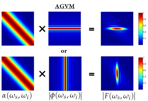
Flin(ωs,ωi) = α(ωs,ωi) × φ(ωs,ωi) (A1.48)
It is the product of two functions:
The energy conservation functionα(ωs,ωi):
α(ωs,ωi) = h ˜ E(+)p ∗ ˜E(+)p i (ωs+ ωi) (A1.49)
The phase-matching functionφ(ωs,ωi): φ(ωs,ωi) = sinc h ∆βlin(ωs,ωi) L 2 i × exp h i∆βlin(ωs,ωi) L 2 i (A1.50)
The obtained linearised JSA expression has the advantage of being more intuitive as it decorre-lates the pump contribution from the one of the medium.
e) Note on the non-degenerate pump scenario
In the case of non-degenerate pumps, an analytical solution of the JSA can also be found with the additional assumption of considering ˜E(+)p1 and ˜E(+)p2 as gaussian pulses of widthσ1andσ2, respectively. In the degenerate pump scenario we did not use any assumptions on the pump spectral shape. As we will not use the non-degenerate regime in this work, we will not derive the calculation but only give the final expression [34].
α(ωs,ωi) = e −(ωs −ωs0+ωi −ωi0)2σ2 1+σ22 (A1.51) φ(ωs,ωi) = MBe−B 2(β linL)2herf( 1
2B− i BβlinL) + erf(i BβlinL) i
(A1.52) where M is a normalization coefficient, erf is the error function and B is defined as B =
p σ2
1+σ22 σ1σ2L(β1p1−β1p2).
In such a configuration, one would have to consider the group velocity difference between the two pumps (β1p1− β1p2 6= 0), which limits the interaction length to the effective distance where they overlap. This is the so-called group-velocity walk-off (contained in the term B).
Conclusion
In this chapter, the analytical expression of the photon pair wavefunction in the degenerated pump regime has been derived. We have shown that it can be written as a product of: (i) a phase matching function (in the form of a cardinal sine function) resulting from the spatial integration over the fiber length and (ii) an energy conservation function (in the form of an autocorrelation of the pump spectrum) resulting from the temporal integration over the total duration of interaction.
1.3. Deriving the Hamiltonian
predicted from the knowledge of fiber parameters (length, dispersion, n2) and the pump pa-rameters (temporal/spectral shape).
We recall however that such derivation is valid only under the assumptions of a weak pump regime so that we can approximate the hamiltonian to its first order Taylor series and neglect the multipair contributions.
The next chapter is devoted to the study of the joint spectral amplitude function which de-scribes the spectral correlations.
Joint Spectral/Temporal Amplitude
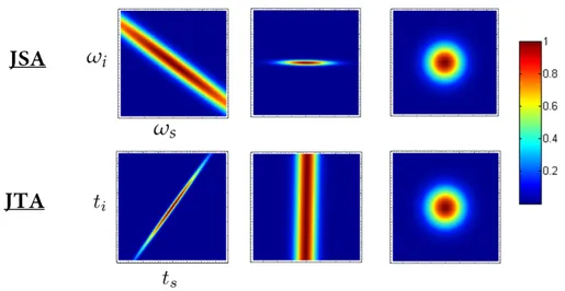
2.1 Joint Spectral Amplitude . . . 31 2.2 Schmidt decomposition . . . 37 2.3 Group velocity matching . . . 43 2.4 Joint Temporal Amplitude and Phase Correlation . . . 46 2.5 The spectral density map . . . 49
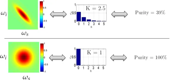
This chapter describes the physical interpretation of the joint spectral amplitude function. It is a powerful tool to describe the joint effects of the pump and the medium. Moreover, a link between this function and the spectral properties of the photon-pairs is discussed. In particu-lar, we will see how this function is related to the time-frequency correlations (= entanglement between the photons of the pairs) and the purity of individual signal and idler photons. In a second section, the Schmidt decomposition is introduced to give a quantitative characteriza-tion of the spectral entanglement and strategies to control the amount of spectral correlacharacteriza-tions are described in the third and fourth sections. The last section presents the spectral density map which is a useful tool to describe the phase-matching as a function of pump wavelength.
2.1 Joint Spectral Amplitude
As described in the last chapter, the state produced by spontaneous four-wave mixing in an optical fiber of length L is given by:
¯
¯ψ® = |0,0〉 + κ Ï
dωsdωiF(ωs,ωi) |ωs,ωi〉 (A2.1)
Where we recall that the quantityκ is a constant corresponding to the generation efficiency, and F(ωs,ωi) is the complex-valued joint spectral amplitude function (JSA), normalised to
2.1. Joint Spectral Amplitude
Î dωsdωi|F(ωs,ωi)|2= 1. Moreover, the JSA can be approximated as the product of the
en-ergy conservation functionα(ωs,ωi) and the phase matching functionφ(ωs,ωi):
F(ωs,ωi) ≈ α(ωs,ωi)φ(ωs,ωi) (A2.2)
Let us discuss in more details the physics contained in each terms of this approximated analytical expression1of the photon pair state:
a) The generation efficiency densityκ
The efficiency of photon-pair generation is related to [29]:
|κ|2≈³n2ωp
c Aeff L Ppτp
´2
(A2.3)
with n2the medium non-linearity, Aeffthe fiber transverse effective area, L the fiber length, Pp
the peak power andτpthe pulse duration of the pump.
The probability to generate a signal photon in the range [ωs0− dωs/2,ωs0+ dωs/2] and an
idler photon in the range [ωi 0− dωi/2,ωi 0+ dωi/2] is given by:
Proba(ωs,ωi) = |ωs,ωi¯¯ψpair® |2dωsdωi (A2.4a)
= |κ|2F(ωs,ωi)2dωsdωi (A2.4b)
F being a normalized function, it is |κ|2that bears the quantitative part of the generation effi-ciency. The quadratic dependence of the generation rate with respect to the pump intensity Pp
favours the use of pump with high peak power2.
In practice, fiber based photon pair sources usually exhibit efficiency in the order of 10−5 to 10−2pairs/pulse for a length in the meter range and a few mW of average pump power with picosecond pulses.
b) Energy conservation functionα(ωs,ωi)
α(ωs,ωi) =
h ˜
E(+)p1∗ ˜E(+)p1i(ωs+ ωi) (A2.5)
This term bears the energy conservation condition, imposing that the energy of the created photons ħωsand ħωicorresponds to the energy of the two annihilated photons around 2ħωp0.
Indeed, since ˜Ep1(ω) is a function of ω − ωp0, it follows thatα(ωs,ωi) is centered aroundωs+ 1please refer to Eq. (A1.41) for the exact expression
2as opposed to SPDC where the brightness increases only linearly with pump power such that both continuous
ωi−2ωp0. The fact that this function embodies the energy conservation function is an expected
result since it is derived from the time integral of the interacting fields and it is well known that energy conservation is related to time invariance. The longer the pulse (= higher time invari-ance), the less the energy conservation is relaxed. In other words, since we consider a pulsed pump, ˜E(+)p1 has a spectral widthσ centered on ωp0. The narrowerσ, the stricter the energy
conservation condition. In the limit of a monochromatic pump3, it can be easily demonstrated thatα(ωs,ωi) tends toδ(2ωp0− ωs− ωi).
Fig. A2.1: Schematics of the energy conservation. Representation on the right shows a more realistic
scheme where, due to the spectral width of the pump, the energy conservation is slightly relaxed.
Let us consider a Gaussian pump amplitude, E(ωp) = E0e− (ω−ωp0)2
2σ2 . Such assumption legiti-mately describes the usual spectrum exhibited by a standard pulsed laser. The autocorrelation of the Gaussian spectrum also gives a Gaussian of the form:
α(ωs,ωi) = E20e−
(ωs +ωi −2ωp0)2
4σ2 (A2.6)
For a Gaussian spectrum the functionα is fully described by two parameters:
• its width∆α related to the spectral width σ of the pump amplitude (∆α =p2σ). • its position in the 2D plane related to the central frequencyωp0of the pump laser
This function can be displayed graphically in the 2D plane (ωs,ωi) to get a better insight of its
physical meaning, as for instance in Fig. A2.2. It is noteworthy thatα function always exhibits a slope of −45°, regardless of the shape of the pump spectrum (Gaussian or not). It comes from the equation: 2ωp0− ωs− ωi = 0. This slope is a signature of the anti-correlation between
signal and idler frequencies, due to the energy conservation.
Moreover, because the FWM comes from the interaction of two pump photons, the energy conservation functionα is the autocorrelation of the pump spectrum. This is different from SPDC where, as only one pump photon is converted,α is directly proportional to the pump
2.1. Joint Spectral Amplitude
Fig. A2.2: Computed functionα(ω,ωi) when considering different parameters of the Gaussian pump
amplitude. The first row shows different spectral widths∆ω for a fixed pump wavelength (λp= 1030
nm) whereas the second row different central wavelengthλp0 for a fixed spectral width (∆ω = 0.12 THz).
spectrum. When considering a standard gaussian pump spectrum, the difference between SPDC and FWM is not really remarkable as the autocorrelation of a gaussian is also a gaus-sian. However notable differences occur when considering non-gaussian pulses. Figure A2.3 shows such an example when considering a square pump spectrum.
Fig. A2.3: Example illustrating the difference between the energy conservation function for SPDC and
for FWM when pumped with a square spectrum pump. The spectra in the right hand side correspond to a projection ofα(ωs,ωi) along the signal axis.
c) The phase matching functionφ(ωs,ωi) φ(ωs,ωi) = sinc h ∆βlin(ωs,ωi) L 2 i × exphi∆βlin(ωs,ωi) L 2 i (A2.7) This third term is the phase matching function which expresses the momentum conser-vation. Indeed the term is maximal when the argument of the cardinal sine function cancels, which happens when 2β(ωp) = β(ωs) + β(ωi). As described, it derives from the spatial integral
of the fields over the fiber length (Eq. A1.35). Once again, this is not surprising considering the well-known link between space invariance and momentum conservation4. Besides, due to the finite fiber length, the momentum conservation is relaxed. The longer the fiber, the sharper the momentum conservation and, in the limiting case where L → ∞, the function would become a delta functionL1δ(2β(ωp) − β(ωs) − β(ωi)).
Fig. A2.4: Illustration of the momentum conservation requirement. In the fiber, the different
momen-tum vectors are parallel to the direction of propagation.
For a given pump energy, an infinite number of frequency pair combination of (ωs,ωi)
fulfil the energy conservation. The medium dispersion determines the likelihood of each of these possibilities through the phase matching condition. In others words, the pump brings the amount of energy available and the medium dictates how this energy is converted.
More quantitatively, if we zoom around a certain coupleω0s andω0i, the main lobe of the sinc can be approximated by a Gaussian of the form5[36]:
¯ ¯ ¯sinc h ∆βlin(ωs,ωi) L 2 i¯ ¯ ¯ ≈ e −γL2¡∆β lin(ωs,ωi) ¢2 (A2.8a) = e−γL2 ¡ (ωs−ω0s).(β1p−β1s)+(ωi−ω0i).(β1p−β1i) ¢2 (A2.8b) withγ = 0.04822.
4an another way to see this is to consider the gain-bandwidth trade-off. For a longer fiber, the gain increases but
then, the bandwidth decreases.
2.1. Joint Spectral Amplitude
Which corresponds to a Gaussian in the (ωs,ωi) plane of width∆φ, making an angle θ
rel-atively to theωsaxis with:
∆φ ≈ 1 L q 2γ¡(β1p− β1s)2+ (β1p− β1i)2 ¢ θ = −arctan(β1p− β1s β1p− β1i ) (A2.9a) (A2.9b)
Importantly, the width∆φ is inversely proportional to the length of the medium L whereas the angleθ is only related to the inverse group velocities β1(ω) =vg1(ω) in the medium. Figure A2.5 shows examples of different values of these two parameters.
Fig. A2.5: Computed |φ(ωs,ωi)| for different parameters. The first row represents modifications of
the width (inversely proportional to the fiber length) for a fixed angle (θ = −10°) and the second row modifications of the angle for a fixed length L. The rebounds are due to the sinc.
One can already observe that the differences inβ1between pump, signal, and idler are a decisive factor in determining the shape of the JSA as it governs the angleθ. Such angle will be crucial when considering the spectral correlations later on (section A2.3).
d) Joint Spectral Amplitude
Writing the JSA as the product ofα and φ nicely separates the pump influence (represented by the energy conservation function) from the medium influence (represented by the phase matching function). Such a separation is useful as we will independently shape the medium