Muscle-Based Control For Character Animation

HAL Id: hal-01317881

https://hal.inria.fr/hal-01317881

Submitted on 18 May 2016

HAL is a multi-disciplinary open access

archive for the deposit and dissemination of

sci-entific research documents, whether they are

pub-lished or not. The documents may come from

teaching and research institutions in France or

L’archive ouverte pluridisciplinaire HAL, est

destinée au dépôt et à la diffusion de documents

scientifiques de niveau recherche, publiés ou non,

émanant des établissements d’enseignement et de

recherche français ou étrangers, des laboratoires

Muscle-Based Control For Character Animation

Ana Lucia Cruz Ruiz, Charles Pontonnier, Nicolas Pronost, Georges Dumont

To cite this version:

Ana Lucia Cruz Ruiz, Charles Pontonnier, Nicolas Pronost, Georges Dumont. Muscle-Based

Con-trol For Character Animation.

Computer Graphics Forum, Wiley, 2016, 36 (6), pp.122-147.

Muscle-Based Control For Character Animation

A. L. Cruz Ruiz1,2, C. Pontonnier1,2,3, N. Pronost4, G. Dumont1,2

1_{IRISA/INRIA MimeTIC, Rennes, France}

2

ENS Rennes, Bruz, France 3

Ecoles de Saint-Cyr Coëtquidan, Guer, France

4_{Université Claude Bernard Lyon 1 - LIRIS SAARA, Lyon, France}

Abstract

Muscle-based control is transforming the field of physics-based character animation through the integration of knowledge from neuroscience, biomechanics, and robotics, which enhance motion realism. Since any physics-based animation system can be extended to a muscle actuated system, the possibilities of growth are tremendous. However, modeling muscles and their control remains a difficult challenge. We present an organized review of over a decade of research in muscle-based control for character animation, its fundamental concepts and future directions for development. The core of this review contains a classification of control methods, tables summarizing their key aspects, and popular neuromuscular functions used within these controllers, all with the purpose of providing the reader with an overview of the field.

1. Introduction

Character animation is the art of bringing virtual characters to life through the design of solutions, such as motion con-trollers, that allow the reproduction and/or synthesis of new motions. The way these solutions are designed depends on the requirements of the specific application for which the character will be used, such as the degree of realism. We de-fine realism as the visual degree of similarity between the ac-tions, motions and responses of virtual characters with those of their real counterparts, at both the dynamic and kinematic level. The desired degree of realism also varies depending on the application. For instance, in a game or simulation, a higher degree of realism is sought for the main characters as opposed to background characters.

In this review, we present a recent, but growing trend, for the production of realistic character animations: muscle-based control. This solution entails the use of more detailed character models, involving muscles and their controllers. Muscle-based models and controllers already span a variety of areas, such as: ergonomic design, rehabilitation therapies, prosthetics, medical diagnosis and even post-surgery predic-tions. In animation, their usefulness no doubt depends on the requirements described above, along with the time to setup the model, and the desired motion repertoire. Nevertheless, we will show that it is a promising direction for the field of character animation in terms of enhancing motion realism. Thus, the main objective of the review is to provide

anima-tors involved in motion control, and experts from other fields (such as robotics and biomechanics) with similar interests, with a wide overview of the field of muscle-based control for animation.

Let us first introduce muscle-based control from a his-torical point of view. Throughout the years, several solu-tions have been proposed to mimic how humans and ani-mals control their motions in order to animate virtual

char-acters [Wil87]. These solutions are split into two main

approaches: kinematic-based methods and physics-based methods. The former involves animating characters by speci-fying limb or joint trajectories. The latter involves animating characters by specifying actuator trajectories, such as joint torques or muscle signals.

One of the earliest kinematics-based methods was keyframing. In this technique the user specified a sequence of positions and their corresponding times, later a computer made an interpolation (usually a splining technique) between the specified positions to generate motion. However, this im-plicated a very low level control, where the user had to con-trol each degree of freedom of the character. Another tech-nique was the use of control functions, where the motion for each degree of freedom was specified via functions of posi-tion versus time, these funcposi-tions were generally curves com-posed of a set of control points. This technique had the ad-vantage that the changes could be more easily made on indi-vidual degree of freedoms, but the control was still very low

level. Later, with the arrival of motion capture systems, ani-mators began using recorded human kinematic data to drive

or enhance animations [PB02] [Gle98]. One major drawback

of this technique was that motion diversity and quality were limited and conditioned by a motion database. Nevertheless, some approaches have extended and diversified the number of motions beyond those of the original databases by apply-ing external forces on the characters and makapply-ing dynamic

corrections on the original motion [MKHK08] [PD07].

A different approach to animation is physics-based anima-tion. This technique is based on the development of physics simulators, which aim at replicating real environments by modeling the physical laws and conditions that define it. This has freed animators from worrying about enforcing certain motion characteristics which come implicitly with the pres-ence of physics, and has granted virtual characters with a freedom of motion, that is unrestricted but physically plausi-ble. Once these virtual environments are created, the tor should choose what character will be used for the anima-tion and a strategy for moanima-tion synthesis (the strategy for the design of a motion controller) .

The character model can exhibit different levels of de-tail in terms of skeleton, actuators and tissues etc. (as will

be explained in section 3). A common choice has been

simple skeletons actuated by ideal servo-motors, and com-manded by servo-based controllers. A very complete re-view and categorization of these controllers can be found

in [GP12]. The animation systems discussed in the

lat-ter review featured motions ranging from 2D locomotion [Hod91] [vdPF93] and forward flips [HR90], 3D

locomo-tion [RM01] [RH02] [Sim94], balance [YLvdP07] [

CB-vdP10] [CKJ∗11] [LKL10] [AdSP07] [MZS09] [WZ10],

and navigation on uneven terrain [WP10] [MdLH10].

Despite these advances, several authors from areas, such as biomechanics, have shown the importance of increasing the level of detail in such models by including muscles as actuators (in the place of servos), and performing a muscle-based control. This has triggered an evolution from servo-based control, to servo-muscle-servo-based control and finally to muscle-based control. Servo-based control assumes that the degrees of freedom (DoF) of the character are actuated by servo motors, and therefore produces torques. Servo-muscle-based control assumes that a set of degrees of freedom is ac-tuated by servos, while another set is acac-tuated by muscles, and consequently it produces a set of torques and a set mus-cle signals. Finally, musmus-cle-based control assumes that all the joints of the character are actuated by muscles and pro-duces muscle signals only.

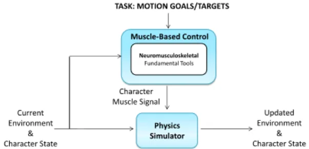
Figure1depicts how muscle-based control is integrated

in a physics-based framework. In this diagram, the physics simulator updates the state of the character and the environ-ment as a result of the external forces in the environenviron-ment and internal forces in the character. The external forces in the environment include gravity, force perturbations, and forces

due to obstacles, slopes, and changes in the friction coeffi-cient. The internal forces in the character are the muscle, lig-ament, and joint-contact forces, which are generated thanks to the muscle signals produced by the muscle-based control method. To design these control methods, knowledge in neu-romusculoskeletal simulation is vital since it provides a ba-sis on which to: model the characters, automate the motion generation process, and solve the motion redundancy prob-lem. More information on these topics will be featured in

section3.

The simulator first gathers the internal and external forces, and executes a forward dynamics simulation that helps to compute the resulting state of the character. This state com-prises several kinematic and muscle variables, such as the position and velocity of each link (or sub-body) in the char-acter, and the length and velocity of shortening or lengthen-ing of each muscle. Specifically, the simulator first computes the link accelerations. These are then fed to a numerical in-tegrator that updates the link positions and velocities, which are finally used to update the state of the muscles.

Physics Simulator Muscle-Based Control Neuromusculoskeletal Fundamental Tools Current Environment & Character State Updated Environment & Character State Character Muscle Signal

TASK: MOTION GOALS/TARGETS

Figure 1: Animation using a muscle-based control frame-work.

As previously mentioned, the main contribution of this re-view is providing the reader with an overre-view of the trends in the field of muscle-based control for animation. We be-gin by explaining our motivation in section 2. In section 3 we present an overview of the neuromusculoskeletal sim-ulation tools, used to design control laws, such as muscu-loskeletal modeling, simulated dynamics and muscle force estimation. The core of the review is section 4, where we feature a muscle-based control method classification consist-ing of two categories: controller optimization methods and trajectory optimization methods. This section also contains the main strengths and weaknesses of each method and ex-amples of controllers found in the animation domain. Next, section 5 features comments on the current and future de-velopments in the field of muscle-based animation. Finally, the review concludes with a set of appendixes including the most relevant aspects presented. Appendix 1 contains a ta-ble summarizing our classification and important control and model features. Appendix 2 contains a list of neuromuscular cost functions used by the controllers. Appendix 3 contains a short list of physics simulators and the controllers that use them.

Lastly, we would like to emphasize that the review aims at highlighting the contributions and novelties introduced by state of the art muscle-based controllers and the characters they use. Therefore, it provides brief but comprehensive de-scriptions of relevant controllers (with a special focus on their muscle-related components). It also provides a general discussion on musculoskeletal modeling, with thorough de-scriptions only of the models these controllers use. For more details on state of the art muscle modeling, the reader is

in-vited to consult [LGK∗10]. We would also like to underline

the fact that most of the frameworks perform muscle-based control, however a few perform servo-muscle-based control, meaning that they involve characters actuated with both ser-vos and muscles. In such frameworks we focus on the muscle controlled part.

2. Motivation

Several studies have shown the importance of considering internal forces when describing joint kinematics, specially in joints where complex interactions between muscle actions, soft tissues and cartilage exist (such as spinal disks,

shoul-ders and knees) [ADR11]. Considering muscles, in

partic-ular, comprises several advantages: better stability

proper-ties and more realistic passive dynamics (section2.1),

bet-ter estimates of energy cost or fatigue (section2.2), efficient

control via motion mechanics (section2.3) and an ease to

simulate musculoskeletal defects, pathologies and physical

fatigue (section2.4). These advantages are a consequence of

the non-linear properties present within the muscles, such as the force-length and force-velocity relationships (these

prop-erties are detailed in section3.1).

Moreover, muscles are at the center of important motor control theories. For instance, the spring-like behavior of muscles has been a crucial part of motor control theories

such as the variants of the equilibrium point theory [

BH-MIG92] [Fel86]. Their coordinated actions also form the ba-sis to theories such as muscle synergies (both theories will

be described in3.4).

2.1. Stability and passive dynamics

The musculoskeletal system is able of achieving

pas-sive adjustments and these adjustments are robust

across certain changes in the environment and

pertur-bations [vdKdGF∗09]. This is due to the fact that the

non-linear properties of muscles grant the body with a first

defense to counteract mechanical perturbations [HR11].

Their presence gives place to adjustments such as preflexes, which are mechanical responses that precede stretch reflexes when a muscle is activated.

The authors of [GvdBHZ98], investigated to what extent

these properties contributed to the recovery from perturba-tions during locomotion by using different models with dif-ferent actuators: servos, muscle models and models

with-out force-length and force-velocity relationships. They con-cluded that the character actuated by muscle models (with both properties) had substantially better resistance to both static and dynamic perturbations. The role of these proper-ties has also been investigated in the control of explosive

movements, such as vertical jumping [vSB93]. The authors

concluded that the force-length-velocity properties of mus-cles were responsible for a reasonable performance when small perturbations were applied.

2.2. Physiological feasibility and energy estimates The inclusion of muscles motivates physiologically

feasi-ble motions. An example of this can be found in [KSK00],

where the physiological infeasibility of interpolating user-input postures was shown, and it was later reduced based on muscle dynamics. Muscles also provide better estimates of

energy expenditure. In [WHDK12], visual, kinematic, and

dynamic comparisons evidenced that walking motions syn-thesized via energy estimates using muscles were closer to real human data than the estimates based on torques. Re-cently, comparisons have also been made between torque actuated and muscle actuated simulations of human

swim-ming [Si13]. The former yielded plausible results but high

control gains and a smaller numerical time step were neces-sary.

2.3. Control via motion mechanics

Thanks to the presence of muscles, the mechanical sys-tem of the character is granted with the ability to accom-plish control functions, not only for counteracting pertur-bations, but also for tasks such as human walking. For in-stance, instead of trying to create control models that mimic complex neural circuits (for either torque or muscle-based characters), biomechanisists have discovered that locomo-tion requires little control if certain principles of legged

mechanics are used. In [GH10], these principles were

en-coded as muscle reflexes, which were used to reproduce human walking, without any higher level controller. These reflexes were inspired in spinal reflexes, which link sen-sory information directly into muscle activations, bypassing the inputs from the central nervous system (such reflexes

will be further described in section3.4). Other authors have

demonstrated that specific mechanical behaviors observed during walking can be encoded in a single, simple muscle

re-flex [PGB97] [GSB03]. Nevertheless, more evidence of the

performance of such legged mechanics principles, in terms of walking on uneven terrain and in various directions, is still needed. This evidence is needed to show the extent to which reflexes can deal with such tasks without a higher level con-troller.

2.4. Simulation of musculoskeletal defects, pathologies and physical fatigue

Among other advantages of muscle-based control is the fact that muscles provide a natural solution to the simula-tion of musculoskeletal defects, pathologies and physical fa-tigue. By taking into account an anatomical structure (mus-culoskeletal system), it is easier to simulate phenomena that derive from this structure. For instance, fatigue and recovery muscle models can be used to simulate a motion where a

hu-man gradually gets tired [KSK00] by limiting the maximal

force that the muscle can produce with respect to the

his-tory of muscle force [GML93] [GML96]. Cost functions that

minimize the force of a specific muscle can be used to

syn-thesize motions with pain avoidance behaviors [LPKL14].

Changing muscle parameters and properties such as max-imal strength, can be used to weaken muscles, and

gen-erate well known pathologies and defects [WHDK12].

Fi-nally, injuries can also be simulated by displacing

mus-cles [KSK00].

3. Neuromusculoskeletal simulation overview

Humans are actuated by muscles controlled by the central nervous system. These muscles produce forces that actuate joints to achieve a given motion. The motion is most of the time realized under external perturbations or forces (such as a voluntary pushes, the force of gravity, and ground reaction forces), which the central nervous system should also com-pensate for.

In the biomechanics field, the neuromusculoskeletal simu-lation can either consist in finding ways to estimate the mus-cle forces from a prescribed motion or directly generating motion from computed forces. The link with physics-based animation is straightforward: by applying to a

musculoskele-tal model (section3.1), an optimal set of muscle forces

(sec-tion3.3) with regard to motion and other requirements, it

should achieve realistically a specified motion.

The following section features a general review of im-portant tools and concepts to understand in a neuromuscu-loskeletal simulation: muscuneuromuscu-loskeletal modeling, simulated dynamics, and muscle forces estimation. Most of the ref-erences cited here come from the field of biomechanics, as biomechanicians are the historical actors of development of the neuromusculoskeletal simulations. However, several openings and applications to animation are highlighted in order to show the strong link between both fields.

3.1. Musculoskeletal modeling

Simulating physics in a system means specifying the seg-ments, joints, masses, inertias and actuation capacities of these systems. Musculoskeletal modeling consists in de-scribing these different features in a convenient way in order to enable a physics simulation. This modeling is common to

different types of virtual characters, such as animals, humans and even imaginary creatures.

3.1.1. Joints and segments

The core problem of musculoskeletal modeling is the definition of anatomically realistic segments and joints. In biomechanics, the models are often anatomically

based [WSA∗02] [WvdHV∗05] and exhibit a higher level

of detail than those used in animation, as they have to be ac-curate enough to provide clinically relevant biomechanical quantities. In many cases, kinematical closed chains appear in the structure of the model and make both kinematics and

dynamics studies more complex [PSVV07] [VDH94].

In the animation field, functional degrees of freedom (i.e. the resulting motion of the anatomical ones) are often

used as a basis for the kinematical model [h-a] and

seg-ments directly link the considered articular centers. Never-theless, some approaches have begun using detailed anatom-ically based models of certain body sections such as the

neck [LT06], hand [SSB∗15], and the upper-body [Lee08].

Using complete body models still remains an area of growth, with only a handful of models presented for mo-tion synthesis purposes, from which the models presented by [Si13] [LPKL14] stand out.

3.1.2. Lengths, masses and inertias

One of the main issues in musculoskeletal modeling is the scaling of the model. As motion is generally recorded to be analyzed (using tracking or motion capture systems), the lengths of the segments are easily computed from marker

positions [LAdZR11]. However, when this information is

not available, regression laws based on cadaver

measure-ments [Dem55] can be used. Cadavers were also used to

scale masses and inertias [dL96] [DCV07]. However,

ad-vances in medical imaging, (e.g. scanner or MRI scanners) opened the door to subject-specific scaling of musculoskele-tal models and showed interesting perspectives for clinical

applications [BAGD07]. Moreover, other approaches have

emerged which rely only on exterior measurements of the body, such as 3D point clouds, to determine subject-specific

bone geometry and motion [ZHK15].

In the models used by the control methods in this review, the parameters are manually specified for every new

charac-ter. However, some exceptions exist, such as [GvdPvdS13]

and [HMOA03], which automatically computed the muscle

parameters by including them in optimization procedures. 3.1.3. Servos and muscles

Historically, as shown in figure2(left), muscles were not

represented and the simulation was mainly skeletal. Estima-tion of joint torques with servo actuated joints was the main goal, but provided no relevant information about muscle load and fatigue. Progressively, muscles were incorporated in the simulation models as non-direct actuators of the joints.

This has also been the case for animation, where charac-ters have evolved in level of detail, and muscle models are finding their way into motion control frameworks. A more straightforward inclusion of muscles began with the use of mass-spring systems. Contrary to the usual angular-spring dampers and PD-controllers, these systems (like muscles) are non-direct actuators of the joints. Meaning, they pro-duce first forces, not torques, which interact with the skeletal system to produce motion. Like muscles, these systems use force action lines, determined by their insertion or attach-ment site to the skeletal structure. Nevertheless, nowadays, more faithful muscle representations, such as biomechanical muscle models, are actively used.

Muscle actuated Servo

actuated

Figure 2: A biomechanical upper limb model. On the left, the elbow is actuated by a virtual servo. On the right, the elbow is actuated by muscles.

One popular biomechanical muscle model that has been incorporated into virtual characters for force generation is

the Hill muscle model [Hil38]. Although this model was

developed decades ago, its current usefulness is evidenced by its various adaptations and implementations within the biomechanics community. These adaptations have come to be known as Hill-type models, such as the Hill-Stroeve

model [Str96], and the widely used adaptation made in

the late eighties by [Zaj89], for numerical simulations. As

shown in figure3, the model consists of a contractile

el-ement CE (non-linear visco-elastic relationship) in parallel with a passive element PE (non-linear spring). The contrac-tile element represents the active tension, or forces, created by the contractile proteins in the muscle, while the passive element represents the passive tension or the force that re-sults from the elongation of the connective tissue compo-nents in the musculotendon unit. The tendon is represented

by a serial non-linear spring SE of length lt, α represents

the pennation angle or the orientation of the fibers with

re-gard to the tendon, lmrepresents the muscle length, and lmt

the length of musculotendon unit. The latter is computed by

adding the muscle lmand tendon ltlengths. This model has

been widely used even if the numerous parameters neces-sary to completely define its behavior are difficult to obtain

in vivo [HKVdH∗07] [IEC10].

The muscle force generation Fmof a musculotendon unit j

can be summarized as the sum of the contractile and passive forces: Fm j= [ fp(lm) + aj· fl(lm j) · fv(˙lm j)] · F0 j (1) 𝛼 𝑙𝑡 𝑙𝑚𝑡 𝐹𝑚 𝐹𝑚 SE

Figure 3: Commonly used musculotendon model for

muscu-loskeletal simulations. Inspired from [Zaj89] [EMHvdB07].

where fpis the passive force relationship, ajis the muscle

activation, fl is the force-length relationship, fvthe

force-velocity relationship, F0 jthe maximum isometric force, and

lm jthe normalized length of the muscle unit (normalization

is usually made using the resting length of the muscle).

Sev-eral models have been proposed to approximate the fl and

fvrelationships with regard to experimental data [RAPC10].

Example models are presented in figure4. The force-length

relationship documents how muscle tension varies at differ-ent muscle lengths, and it is related to the "Sliding Filamdiffer-ent Theory". At a microscopic level, muscle fibers are composed of smaller structures called actin and myosin filaments that make bindings to form muscle contractions. Peak muscle force can be generated when most of these bindings or cross-bridges are created. This event corresponds to the resting length of the muscle (usually near the middle of the range

of motion) [Knu07]. The force-velocity relationship explains

how the force of fully activated muscle varies with velocity. It states that the force the muscle can create decreases with increasing velocity of shortening (concentric actions), while the force the muscle can resist increases with increasing

ve-locity of lengthening (eccentric actions) [Knu07].

The tendon force fjt, output of the musculotendon unit, is

simply obtained by taking into account the pennation angle:

fjt= Fm j· cos αj (2)

However, in many studies the pennation angles are ne-glected.

Complete dynamics of the musculotendon unit also in-cludes the activation dynamics, meaning that there is a non-linear temporal relationship between the neural excitation

uj and the effective activation of the muscle [BLMB04].

In many works [VYN05] [VYN06] [PD09], this non-linear

1 𝑙 𝑚 0 1 0 𝑙 𝑚 1 0 Force-Velocity relationship 𝑓𝑣 Force-Length relationship 𝑓𝑙 Contractile element CE 𝑙 𝑚 0 0 Passive element PE 1 Passive force relationship 𝑓𝑝

Figure 4: Force generation capacity of muscles. Inspired

from [RAPC10] [EMHvdB07].

equation, exhibiting different time constants for activation and deactivation: ˙ ej= (uj− ej)/τne ˙ aj=    (ej− aj)/τact , e≥ a (ej− aj)/τdeact , e< a (3)

Where uj is the neural excitation, aj the muscle

acti-vation, ej an intermediate variable, τne the neural

excita-tion constant time (often neglected), and τactand τdeactthe

activation and deactivation time constants respectively. In animation, activation dynamics is sometimes modeled

us-ing equal activation and deactivation time constants [

Gvd-PvdS13] [WHDK12].

The musculotendon unit modeling remains challenging, since changes in the tendon length affect the final muscle force, and vice-versa. A proper evaluation of the muscle

length should be done [MD12]. However, such a

computa-tion is costly in terms of computacomputa-tion time and is often

sim-plified. For example, the algorithm used in [DRC∗06] just

it-erates once at each simulation time step, assuming that most of the tendon effect will be obtained with only one iteration. Besides the mechanical model presented previously, other muscle models have emerged which encompass vi-sual characteristics such as muscle deformation or both

functional and visual characteristics [LGK∗10]. The

mod-els can be grouped under three techniques: geometrically-based, physically-based and data-driven approaches. In geometrically-based approaches, muscle deformation is

de-termined by the skeleton arrangement [CHP89] [WVG97]

[TSC96]. In physically-based approaches both the

con-tractile muscle forces and the changing muscle

geome-try are represented during contraction [NTH01] [TZT09]

[TSB∗05]. Finally, data-driven approaches directly model

the skin shape that is deformed by the underlying muscle,

thanks to data captured from the surface of subjects [ACP03]

[PH06] [FLP14]. These models offer a next level of fidelity. However to this date they are not usually used for the control of virtual characters due to the fact that they would render the control computationally expensive.

3.2. Simulated dynamics

As it has been stated in [EMHvdB07], the musculoskeletal

dynamics problem can been presented as follows: let us con-sider a musculoskeletal system with n degrees of freedom, actuated by m muscles. The degrees of freedom are the joint angles gathered in a vector called q. The state of such a mus-culoskeletal model, from a dynamics point of view, can be

expressed as (q, ˙q).

The relationship between motion and forces is given by the Newton’s second law of motion, that can be expressed in

a matrix form as [Pan01]:

M(q) ¨q+ C(q, ˙q) + G(q) + R(q)Fm+ E = 0 (4)

Where M(q) is the mass matrix of the system,

gather-ing masses and inertias of all the segments (n × n), C(q, ˙q)

represents the coriolis and centrifugal effects (n × 1), G(q) represents the vector of gravity torques (n × 1), and E

rep-resents the external forces. Finally, R(q)Fm represents the

action of the muscles on the joints (muscular joint torques,

n× 1) , where R(q) is the matrix containing the muscular

moment arms (n × m) and Fmthe muscle forces (m × 1). In

a dynamics simulation, such quantities can be automatically constructed by using algorithms such as the ones developed in [KL96] [Fea14].

From equation4, two different problems can be derived.

The first one, called inverse dynamics, consists in applying a specified motion and specified external forces to a muscu-loskeletal model and then computing the forces that generate the considered motion. The equation to solve is a

reformula-tion of equareformula-tion4and can be expressed as:

R(q)Fm= −(M(q) ¨q+ C(q, ˙q) + G(q) + E) (5)

The output of equation5are the muscular joint torques

that are used to define muscle forces. This equation is most of the time solved thanks to a top-down strategy also referred

to as Newton-Euler algorithm [Win05] [Fea14] [RHWZ08],

which considers each segment separately from distal to prox-imal. However, more robust methods and methods consider-ing closed loops have also been validated to solve the

in-verse dynamics problem [Kuo98] [vdBS08]. This approach

a very common resource and can be used as a kinematical input in such problems.

The second problem is called forward dynamics and is the one that interests us the most, as it consists in generating motion from computed forces. Since no direct measurement of muscle forces is available, this approach is generally cou-pled with an optimization problem to compute a set of forces compatible with a given task. The equation to solve, issued

from equation4can be written as follows:

¨

q= M−1(q)(−C(q, ˙q) − G(q) − R(q)Fm− E) (6)

In animation, the forward dynamics problem is incorpo-rated in a physics simulation involving collision detection (that provides external forces to apply to the system) and a numerical integration (e.g. Runge-Kutta methods) to obtain

the current system state (q, ˙q) from the computed

acceler-ations ¨q. In biomechanics, the problem is generally solved

with real external force measurements (such as ground re-action forces from force plates), and it is formulated as the optimization problem presented in the next section.

3.3. Muscle forces estimation

Most musculoskeletal models exhibit actuation redundancy (m > n) that leads to an infinite number of actuation solu-tions, as there are less equations (dynamics equations) than unknowns (muscle forces). The models may also exhibit un-deractuation, which stems from the fact that a single muscle can actuate several joints simultaneously, such as bi-articular muscles.

These challenges can be solved by defining what is the op-timal actuation solution, through the modeling of known mo-tor control laws associated to a motion. Momo-tor control is the process through which humans and animals create motions by using their neuromuscular system. This process involves the computation of higher level commands by the central nervous system to achieve specific motion goals based on sensory information regarding the environment and the cur-rent body state. These commands later excite the muscular

system, creating skeletal motion [Ros91]. Several models

that mimic this process are actively studied and used in the fields of neuroscience, biomechanics, and robotics to gener-ate muscle forces.

3.3.1. Problem formulation

A popular motor control model is the minimization of a cost function ( f (X )) encoding task goals and bio-inspired objec-tives that motivate natural motion. A common formulation of this model consists in a non-linear constrained optimization problem:

Find X which minimizes f (X ) (7)

subject to, gj(X ) ≤ 0, j = 1, 2, ..., m hk(X ) = 0, k = 1, 2, ..., p Where the constraints enforce that:

• the computed forces solve the dynamic equations; • the muscles are only pulling and they have

physiological-based force limits;

• the computed forces may respect any additional set of uni-lateral (g) or biuni-lateral constraints (h).

The constraints gj(X ) and hk(X ) may be specified as hard

constraints (as in the formulation above), or as soft con-straints (as additional cost functions). The optimization can be a static or dynamic one (often an optimal control

prob-lem [ZDG∗96]). A static optimization refers to the process

of minimizing or maximizing an objective function at a time instant, while a dynamic optimization refers to the process of minimizing or maximizing an objective function over an interval of time of non-zero duration.

3.3.2. Forward, inverse and hybrid dynamics-based optimization

This model can be used both in a inverse dynamics and for-ward dynamics framework. General schemes of these

frame-works are featured in figure5and in figure6.

In the inverse dynamics-based optimization (figure 5),

motion and external forces are applied to a musculoskele-tal model. The generated joint torques are then used in an optimization procedure that computes the muscle forces that satisfy the task, motion objectives, and constraints. In biomechanics, the inverse dynamics problem is often solved by minimizing a cost function representing an

en-ergetic cost [TBB97] [Pan01] [EMHvdB07] [PD09].

Sev-eral cost functions have been tested. The sum of the squared and cubed muscle forces have been classically used for

gait [CB81] and upper arm [AKCM84] [Cha97] motions

as an image of the metabolic energy consumption, whereas

a min/max criterion [RDV01] has been widely used in

er-gonomics applications as an image of the muscle fatigue. These examples are of importance as they are influencing the cost functions that are currently used in the muscle-based animation field. A widely used commercial software exploiting such a method for musculoskeletal analysis is

AnyBody [DRC∗06]. One of the purposes of using inverse

dynamics-based optimization for animation is to provide characters with a certain degree of adaptability to perturba-tions. Computing muscle forces from motion capture data is also interesting because it allows the simulation of new motions (e.g. fatigued or injured motions), by replaying the computed muscle forces while altering muscle

param-eters [KSK00] [WHDK12] [LPKL14]. Moreover, recent

de-velopments allow the computation of these muscle forces

in real-time [vdBGEZ∗13]. Finally, it is worth noting that

the muscle-based variation of jacobian transpose control [SADM94] [GvdPvdS13], which does not use the complete inverse dynamic model, but a simpler, static equivalent. Es-sentially, it consists in finding a set of forces and torques in the task space which achieve a target pose, and converting these into individual muscle torques and excitations via the jacobian transpose.

In the forward dynamics-based optimization problem

(fig-ure 6), only initial muscle excitations and external forces

are applied to the model (no pre-recorded motion). The de-sired motion is instead directly provided to the optimization procedure to evaluate task achievement, and produce the re-quired muscle excitations. Usual cost functions are the dis-tance between computed kinematics (issued from the for-ward dynamics problem) and experimental kinematics data. A good example of a forward dynamics optimization is the Computed Muscle Control algorithm (CMC) implemented

in OpenSim [DAA∗07]. Its forward simulation uses a cost

function that can be based on the distance to experimental data, or on the distance to predefined poses issued from a planner.

Several Hybrid dynamics methods also exist, trying to use the advantages of both methods to be mechani-cally and physiologimechani-cally consistent. These methods ba-sically consist of a inverse dynamics-based optimiza-tion, with the difference that (as in the forwards dy-namics problem) initial excitations are provided for some muscles through the use of electromyographic

measure-ments [BLMB04] [AM04] [ARB10]. The advantage of such

approach is that the dimension of the original problem is re-duced by removing variables from the optimization problem. Numerous optimal control methods have also been devel-oped to obtain realistic motions from scratch through the

ac-tuation of a musculoskeletal model [Pan01] [AvdB10]. This

is also of great interest for the animation field, as optimal control theory is especially well fitted to synthesize a mo-tion between two body poses.

As previously shown, a central and important component in these frameworks is the choice of the objective function. For this reason, we have grouped the most relevant objec-tive terms used in animation according to the categorization

found in [ZW90]. In this categorization, a generalized

per-formance criterion was proposed, which included three com-ponents: task specific (tracking a given trajectory, minimiz-ing jerk), neuromuscular (minimizminimiz-ing muscle stress, neural effort), and bone joint (minimizing contact forces, avoid-ing certain ranges of motion) objectives. Appendix 2 con-tains a detailed description of each of these components and a table listing relevant cost functions. A special focus has been given to the neuromuscular objectives, which represent a novelty in muscle-based control. The reader is invited to consult the reference of each controller for more detailed de-scriptions on the remaining objective types.

To solve the optimization problem, popular algorithms

such as sequential quadratic programming (SQP) [KSK00]

[ZCCD06] [Si13] and simplex methods have been imple-mented. SQP consists in modeling the non-linear optimiza-tion problem as quadratic subproblems and to use the so-lutions of these subproblems to find better approximations

that lead to the optimum [RR09]. If the optimization is

un-constrained, other authors have opted for simpler methods

such as the simplex method [GT95] [DZS08]. This iterative

method uses a geometric shape or simplex to explore the

so-lution space and find an optimum [RR09].

Evolutionary algorithms [dG04] have also been

re-cently incorporated into the control of virtual

charac-ters [HMOA03] [WHDK12] [GvdPvdS13]. An example is

the covariance matrix adaptation (CMA) [Han06], which

uses a multi-variate normal distribution to explore the so-lution space in search of an optimum.

3.4. Motor Control Theories

The optimization itself can be used as a controller to gener-ate muscle signals, or it can be used to optimize bio-inspired control laws based on motor control findings and theories

(Section4.1) such as: hierarchical systems, central pattern

generators, equilibrium point theory, muscle reflexes and muscle synergies. The current section briefly presents these theories and some of the application cases found in both biomechanics and animation.

Hierarchical control systems, have been designed thanks

to studies [KSJ∗00] that outline how the components or

neu-ral organs of the motor system work together to generate muscle excitations for voluntary and reflexive actions. This hierarchy has inspired multiple level controllers in

anima-tion, as in [ZCCD06].

Central pattern generators (CPGs) have been proposed

for the generation of locomotion, and other kinds of be-haviors (such as respiration and swallowing). CPGs are biological neural networks that produce rhythmic patterns without relying on sensory feedback or higher control

cen-ters [Hoo01]. This neural rhythmicity is generated from

teractions between neurons or between currents within in-dividual neurons. Although these networks do not rely on sensory feedback, higher control centers use this feedback to modulate the CPG outputs. The CPG models created by [Tag98] [TYS91] for bipedal locomotion have been

popu-lar in the robotics domain [Ijs08] [AT05] [AT06] [ENMC05]

and are also beginning to be present in the world of an-imation, specifically for the synthesis of human

swim-ming [Si13] and walking [HMOA03]. Nevertheless, a

limi-tation of these generators is the fact that they only produce a limited set of motions, mainly rhythmic or periodic patterns. Using CPG-based methods alone is not enough to provide a character with a rich motion repertoire. For this reason, in applications requiring periodic and non-periodic motions, it is necessary to use an additional control strategy to handle

Updated muscle forces Joint torques Computed joint coordinates Initial muscle forces

Bone lengths, masses and inertias

Motion capture data External force data

Pre-processing Optimization loop

{X, Y, Z} {E} { , , }q q q Inverse dynamics Scaling Inverse kinematics {m} min max min ( ) Subject to ( ) ( , ) 0 ( , ) 0 m m m m m m f f F R q F F F F g F q h F q        {Fm} {Fm}

Optimized muscle forces

{Fm}

Figure 5: Inverse dynamics-based optimization. The optimization problem iterates until the cost function is minimized and the

constraints are satisfied. Adapted from [EMHvdB07] [PDZS∗14].

Computed joint coordinates

Initial muscle excitations

Updated muscle excitations Bone lengths, masses

and inertias Experimental joint

coordinates _{External force data}

Pre-processing

Muscle forces

Optimization loop

Optimized muscle excitations

exp exp exp

{q ,q ,q } {E} { , , }q q q { }em {Fm} exp min ( ) Subject to 0 1 (e , ) 0 (e , ) 0       m m m f f q q e g q h q Forward dynamics Scaling { }em { }em

Figure 6: Forward dynamics-based optimization. The optimization problem iterates until the cost function is minimized and the constraints are satisfied. Excitations are often computed instead of forces for a more straightforward inclusion of muscle dynamics within the solution (activation and force generation properties are highly influential in high performance motions).

Adapted from [EMHvdB07].

Control laws based on the equilibrium point theory [Fel66] have been also implemented by animators [NF02]. This theory argues that the nervous system controls move-ment through the specification of final equilibrium positions of the limb. The equilibrium trajectory mirrors properties of the limb and neuromuscular system, such as inertia and viscoelasticity. This trajectory is specified by virtual posi-tions corresponding to variaposi-tions in muscular activaposi-tions. The muscle activations move the limb from its real position to the virtual one.

Lower level control laws, such as muscle reflex

mod-els [GH10] have recently started to be incorporated into

character motion synthesis, as we will see in the next

sec-tion [GvdPvdS13] [WHDK12]. The models suggested that

reflex inputs (which serve as mediators between the CNS or central nervous system and mechanical environment)

dom-inate in contributions to muscle activations during locomo-tion. This supports the idea that the function of CPGs may be limited during normal locomotion. These reflexes have been included in animation as positive feedbacks of muscle fiber

length and force [GSB03] that altered muscle activation. The

effects of such reflexes was a reliance on compliant leg be-havior, joint overextension avoidance, and improved gait sta-bility.

Finally, a promising theory (somewhat close to the idea behind CPGs), that is yet to be actively applied within animation frameworks, is the theory of muscle synergies. This theory proposes that by combining a few modules, the CNS may learn new control policies fast and efficiently, for instance, to adapt to perturbations. Evidence of this modular organization has been found thanks to the low

such modules has been shown in human arm reaching

mo-tions [MBdF10], human postural responses [TOT07],

over-head throwing [CRPSD15], and frog kicks [dSB03].

All of these theories are of interest since they have in-spired many of the control methods used in animation. In

section4.1we will see how central pattern generators,

mus-cle reflexes, and the equilibrium point theory have inspired

controllers in animation. In section4.2we will show other

control methods which take more inspiration on the work done in the domain of control and robotics. Nevertheless, a handful of these methods have also been inspired by motor control theories, such as the theory of muscle synergies.

4. Muscle-based control methods

Once the character is designed using the musculoskeletal modeling and simulation dynamics concepts presented in

section3.1and section3.2, a muscle-based controller can

be constructed using the force estimation frameworks and

techniques featured in section3.3, particularly, the forward

dynamics-based optimization framework. As initially shown

in figure 1, the purpose of the muscle-based controller is

the computation of adequate muscle signals (muscle exci-tations or muscle forces) that allow the character to achieve a set of tasks and motion goals. Specifically, we are

inter-ested in defining a controller to determine the forces Fmin

equation6.

The motion goals for these controllers can consist of high-level goals, such as walking speed and direction, or task space and joint trajectories. Therefore, the specification of detailed motion data is not a necessity. In fact the purpose of designing controllers is to be as independent as possible from motion data. In the first case, one sole procedure com-putes both kinematics and muscle signals from the high-level goal. In the latter case, either a higher level controller com-putes the desired kinematics and a low-level muscle con-troller transforms it into muscle signals, or the animator pro-vides the kinematic trajectories.

We have grouped the controllers into two categories:

con-troller optimization methods (section4.1) and trajectory

op-timization methods (section4.2). In the controller

optimiza-tion methods, the optimizaoptimiza-tion seeks to determine the opti-mal control parameters that will allow a control law to pro-duce muscle signals that satisfy specific motion goals. Once these parameters are determined, the controllers convert de-sired kinematic goals into muscle signals. These control laws are based on the motor control findings and theories

dis-cussed in section3.4. In trajectory optimization methods, the

optimization directly generates the muscle signal trajectories that accomplish the desired motion goals. Both methods at-tempt to optimize motions with sometimes similar cost

func-tions (Table2), but the controller optimization methods

ac-cess the equations of motion implicitly through experience. In other words they see the character and its environment

as a "black box", while the trajectory optimization meth-ods access these equations explicitly. Furthermore, the con-troller optimization approaches have the characteristic, that (when needed) instead of computing the complete inverse dynamic model, many use a "simpler" equivalent, such as

the jacobian transpose [SADM94] (section3.3.2). Finally,

it is worth noting that to compute the muscle signals, the controller optimization methods perform the optimization offline, while the trajectory optimization methods perform it online.

A section has been devoted to each control method. Each section consists of a description of the control method, its main strengths and weaknesses, and examples from the ani-mation field. Appendix 1 resumes these characteristics for all controllers discussed in this review, and appendix 2 summa-rizes the details and formulas describing the neuromuscular cost functions used by each controller.

4.1. Controller optimization methods

Controller optimization methods seek to determine a set of control parameters that will yield the desired motion goals throughout an entire period of time. These parame-ters depend on the specific control law, but in general they can be summarized as: feedback control law gains (such as PD controller gains, force feedback gains and spring gains) and CPG unit weights. An overview of such methods

is featured in figure7. Animators specify the desired task

( ftask(t)), neuromuscular ( fneuromuscular(t)) and bone joint

objectives ( fbone, joint(t)), constraints (g(sm, q), h(sm, q)),

ex-ternal forces (E), initial control (pm) and character state (sm),

and finally an initial guess of the joint trajectories that fulfill the task. An optimization procedure continually updates the controller parameters and desired joint trajectories until the cost function is minimized. It is worth noting that the final desired joint trajectories might be specified by the animator,

or synthesized by the optimization as in figure7.

Once the control parameters and joint trajectories have been determined, the control law executes online and di-rectly generates the actuation signals that accomplish nat-ural looking motions, while satisfying task related objec-tives. Example of control laws include: antagonistic control, PD-controllers, muscle reflexes, and neural networks. The variety of motions that have been synthesized encompass

human locomotion (ex. walking, running, hopping) [

Gvd-PvdS13] [WHDK12] and postural adjustments [NF02]. 4.1.1. PD controllers and muscle reflexes

Several approaches have made use of the fact that

hu-mans minimize muscle effort during locomotion [R∗76]

within their controller optimization frameworks. Some

no-table examples are the controllers developed by [WHDK12]

and [GvdPvdS13] for synthesizing locomotion in humanoids

Optimal control parameters Optimal desired joint coordinates Updated Computed joint coordinates Muscle signal Updated Muscle forces

Offline optimization tuning loop

{ , , }q q q {Fm} , int max min ( ) ( ) ( ) ( ) Where 0 Subject to 0 1 (s , ) 0 (s , ) 0         

task neuromuscular bone jo

m m m f t f t f t f t t t s g q h q Forward dynamics Muscle control _{{s }} m {p }m {p }m {q q qd, d, d} {q q qd, d, d} {p }m {q q qd,d,d} Initial muscle

signal External force data

{E} Initial desired joint coordinates Initial control parameters Task: Goals/targets {s }m Computed joint coordinates Muscle signal Muscle forces { , , }q q q {Fm} Forward dynamics Muscle control _{{s }} m

Online control loop

Figure 7: Controller Optimization Scheme. The tuning process, which is usually made over a group of time steps [GvdPvdS13],

is iterated until the cost function is minimized or the desired motion is obtained (the tunning process may also consist of a locally

weighted regression [Si13] or manual parameter and target specification [NF02]). The optimal parameters and joint trajectories

are then used in an online closed control loop (instead of joint trajectories [WHDK12] desired muscle lengths [Si13] might also

be used).

optimization procedure to determine the optimal control pa-rameters of PD controllers (PD gains) and muscle reflexes (force and length feedback gains). The optimization had a time horizon of 10s or 20s, and was based on a mus-cle effort term called the rate of metabolic energy

expen-diture [And99], and soft constraints to track kinematic

ob-jectives and ensure stable gaits.

The PD control laws and muscle reflexes generated the muscle excitations to make the character fulfill the

locomo-tion tasks. [GvdPvdS13] used task space PD controllers on

different body segments, inspired by the jacobian transpose

control of [SADM94], while [WHDK12] employed them on

each muscle in the character.

Figure 8: Locomotion of muscle-based bipeds [GvdPvdS13]

These PD controllers worked jointly with the muscle

re-flexes designed by [GH10]. The reflexes encoded principles

of legged mechanics, such as natural joint compliance in

stance phase and dorsiflexion during the swing phase. In ad-dition to these control laws, constant excitations were also used to adjust the output of these control laws according to the gait phase, or to produce rhythmic arm and tail

move-ments. Figure8features examples of the variety of creatures

and motions synthesized by [GvdPvdS13]. Interestingly, in

this approach, the muscle routing of the creatures was also optimized such that the task was successfully achieved. 4.1.2. PD controllers and neural networks

Recently, PD controllers have also been included for synthesizing human swimming motions. The authors of [SLST14] [Si13] used a controller optimization method for periodic motions in swimming, and trajectory

optimiza-tion (consult secoptimiza-tion4.2) for non-periodic motions. The

con-troller optimization method consisted of neural networks (central pattern generators or CPGs) for specific body sec-tions and PD controllers. As opposed to the PD controllers in the previous sections, in this approach, the control gains were fixed, and the parameters in the optimization were a set of weights in CPG model.

The character’s body was divided into 10 muscle groups (ex: right leg, left leg muscles) for the CPG modeling. Each CPG was modeled as a set of non-linear differen-tial equations, that contained desirable properties such as trajectory reproduction, modulation, and external perturba-tion compensaperturba-tion. The networks produced desired

time-varying muscle lengths for specific swimming modes, and the PD controllers converted them into muscle activations. The learning process of these networks was carried out by an

Incremental Locally Weighted Regression (ILWR) [SA98].

This process sought the minimization of an error criterion based on the desired muscle lengths obtained from kinematic data of swimming.

The use of muscle groups, and a higher level controller to modulate each CPG, simplified the control task. For in-stance, turns were induced by decreasing the activation am-plitudes of the muscles on one side of the body relative to muscles on the opposite side.

4.1.3. Antagonistic control

The authors of [NF02] used this methodology, on a

con-troller based on the equilibrium point hypothesis proposed in [Fel66] and introduced in section3.3. However, an alter-native to optimization was used in order to determine the set of parameters that achieved the desired motion. In this ap-proach, each degree of freedom of a human skeleton was ac-tuated by two angular springs representing the antagonistic grouping of muscles around joints. Movement was achieved by varying the equilibrium point of each joint; the equilib-rium point was defined as the point where the sum of the forces acting on the joint equaled to zero. The variation of the equilibrium point was made by adjusting the spring pa-rameters according to desired angles specified by the anima-tor and a method that took samples of external forces and recalculated the parameters.

4.1.4. Summary

Similarly to controller optimization methods in the joint space, these controllers have generated impressive results in terms of skills (list of possible motions of the character) and robustness to external perturbations. However, because mus-cles are used instead of servos, new cost functions (such as muscle effort) have been included within the parameter opti-mization procedure, which further motivate motion realism. These improvements have been evidenced at both the

kine-matic and dynamic level by [WHDK12].

Controller optimization methods have allowed the imple-mentation of models of biomechanical mechanisms. The use

of these laws, such as muscle reflexes [GH10], have

gener-ated well-known events during walking, such as joint com-pliance in stance phase, and dorsiflexion during the swing

phase [WHDK12] [GvdPvdS13]. This represents an

impor-tant advantage, since bio-inspired control laws can directly generate desired muscle and joint behavior at specific stages during the motion.

One of its main drawbacks is computational efficiency. Computation times still need to be improved, since to syn-thesize 10 seconds of animation, the controllers yielding the most impressive results require approximately 10 hours of

tuning [WHDK12]. Nevertheless, we believe that

consider-ing and modelconsider-ing muscle groups and synergies (section3.4)

could aid in overcoming this setback, by explicitly establish-ing relationships among muscles and reducestablish-ing the number of

control parameters [ADN∗13].

Finally, another interesting aspect of some of these con-trol frameworks was the strategy used for ensuring balance

of the characters. For instance, in the case of [GvdPvdS13],

trunk stability was maintained by using feedback rules to control orientation in sagittal and coronal planes with re-spect to the center of mass velocity and a target heading. Balance was also enforced thanks to the application of a

SIMBICON-style balance correction [YLvdP07] to

deter-mine leg orientation in the sagittal and coronal plane. The

authors of [WHDK12] also made use of the SIMBICON

balance feedback laws to adjust desired hip target angles.

Lastly, the approach developed by [NF02] used automatic

balance controllers based on ideas from the balancing

simu-lations of [Woo98].

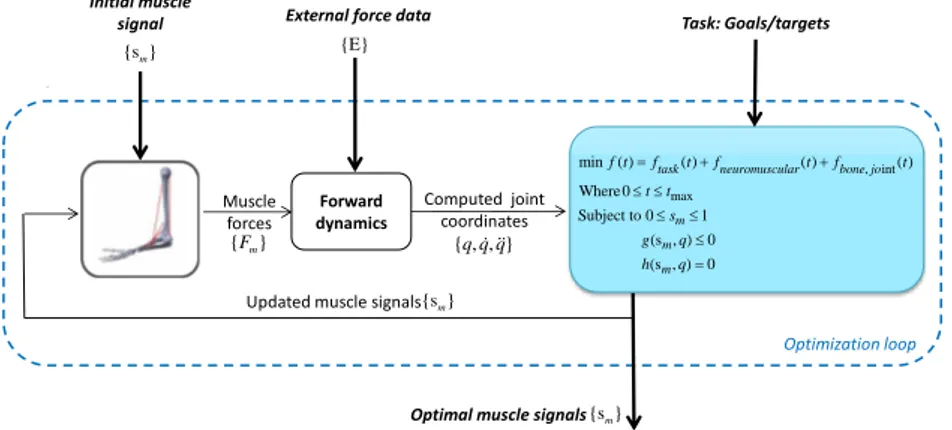
4.2. Trajectory Optimization Methods

The objective of trajectory optimization methods is to gener-ate control variable trajectories that minimize or maximize a measure of performance while also respecting a set of con-straints. Such methods are for now mostly used in robotics. In the domain of character animation, these methods remain mostly a static optimization, solving a given set of equations at each discrete step. Alternatively, they can also be referred to as "model-predictive control methods" when they are used online and with a finite time horizon.

As detailed in section3.3, these optimizations are usually

formulated as non-linear constrained optimization problems that use bio-inspired cost functions, such as muscle effort or muscle fatigue. A schematic overview of this approach

is featured in figure9. Generally, the animator specifies the

desired task ( ftask(t)), neuromuscular ( fneuromuscular(t)) and

bone joint objectives ( fbone, joint(t)), external forces (E), and

initial muscle signals (sm). The optimization iterates until the

cost function is minimized, producing the optimal muscle signals that fulfill the task.

Among the variety of motions that have been syn-thesized through this approach are, locomotion patterns [Mil88] [GT95] [GTH98] [KSK97] [MWTK13] [TTL12], and human upper body movements such as

breath-ing [ZCCD06] [DZS08], arm flexion [LST09], and hand

movements [SKP08] [AHS03].

We have distinguished two types of trajectory optimiza-tion methods: those that rely on the assumpoptimiza-tion of a specific function (periodic or polynomial functions) as a control tra-jectory, and those that don’t. The following sections explain each type and provide further insight into how these con-trollers are used in animation.

Computed joint coordinates Muscle forces { , , }q q q {Fm} Forward dynamics Task: Goals/targets External force data

{E} Initial muscle

signal

Optimization loop

Optimal muscle signals {s }m

{s }m

Updated muscle signals {s }m

, int max min ( ) ( ) ( ) ( ) Where 0 Subject to 0 1 (s , ) 0 (s , ) 0         

task neuromuscular bone jo

m m m f t f t f t f t t t s g q h q

Figure 9: Trajectory-Optimization methods. The optimization process directly computes the muscle control signals according to the minimization of a cost function and targets. These signals can be computed at each time step (static optimization) or in a defined simulation period (dynamic optimization or optimal control). Some approaches include additional components, such as

neural networks to generate the desired joint stimuli [HMOA03] [LT06].

4.2.1. Trajectory optimization based on function primitives

One of the simplest motion control strategies consists in syn-thesizing motions through the generation and tuning of peri-odic signals. These controllers are mainly used for the gen-eration of oscillatory motions, such as those seen in the loco-motion of fishes, worms, snakes and in human chest loco-motions. These signals generally drive spring-like muscles, which are gathered into muscle groups to reduce the number of con-trolled variables.

Early implementations manually tuned periodic functions

to generate the desired motions [TT94] [Mil88] [ZCCD06].

[TT94] controlled artificial fishes by converting a desired

swim speed into a spring contraction amplitude and fre-quency. This mechanism was based on the observation that the speed of most fishes can be proportional to the amplitude and frequency of the tail’s lateral oscillation.

The authors of [Mil88] used controllers that produced

sine waves to generate waves of compression, which repli-cated the elastic deformation present in the locomotion of snakes and worms. Sine waves have also been used jointly

with step functions to generate human motions. [ZCCD06]

used these functions as varying parameters to synthesize hu-man breathing. The first parameter was a contraction ratio, which was determined according to modeled and measured human muscle contraction ratios during breathing. The sec-ond parameter was a binary timing, which was defined by the desired breathing frequency. Finally, polynomial func-tion primitives, such as spline curves, have also served as

a means for human motion synthesis. [AHS03] synthesized

hand motions in real-time by specifying muscle contraction values at keyframes and interpolating them via spline func-tions.

Recent implementations have automated the generation of periodic functions by using optimization procedures. An

ex-ample is the torso controller of [DZS08] for synthesizing

hu-man breathing and laughing. In this approach, an optimiza-tion attempted to minimize the tracking error between a de-sired lung pressure, computed from an audio soundtrack, and the current pressure of the model. This process generated the parameters of a set of sine waves that were used directly as muscle activation signals.

More complex motions have also been synthesized with the use of function primitives. An example is the approach

of [MWTK13], where control trajectories were encoded

as splines, and trajectory optimization and spacetime

con-straints [WK88] were used for humanoid motion synthesis.

The optimization generated joint coordinates, muscle acti-vation signals and lengths, foot contact points, and ground reaction forces. This process was driven by a muscle

ef-fort term (metabolic energy expenditure [AP99]), and

ad-ditional objectives that enforced the equations of motion and encoded other desired muscle behaviors. Although con-tact points and ground reaction forces, which usually in-troduce discontinuities into the optimization, were included in the optimization, this approach was still able to achieve impressive computation times. The reason behind this was the use of the Contact Invariant Optimization (CIO)

frame-work [MTP12]. The framework smoothed out the

discon-tinuities in the objective function by allowing foot contact points to gradually invoke ground reaction forces at a dis-tance until a real contact was made.

Other approaches have begun incorporating motor

con-trol theories, such as muscle synergies (section3.4), coupled

with static optimization. This is the case of the

synergy-based controller for throwing motions developed by [

ex-tracted from human throwing motions and used to actu-ate the character. Next, a synergy-based forward dynamics pipeline ensured that the desired throwing motion was re-produced. The pipeline achieved this through two adapta-tion stages: the first stage consisted in determining the char-acter’s unknown muscle parameters; while the second stage consisted in modifying the time-varying part (or shape) of the synergy via a static optimization, such that the desired throw was reproduced. An interesting feature of this con-troller, was that muscle redundancy was reduced, and that the initial synergies were able to reproduce general trends in the throwing motion.

4.2.2. Trajectory optimization without function primitives

The majority of trajectory optimization methods discussed in this review do not make assumptions on the trajectory of the control signal, and rely more heavily on biomechanical and motor control concepts, such as the minimization of effort or fatigue. We will first discuss the controllers whose sole pur-pose is synthesizing rigid body motions; next we will intro-duce the controllers that also model the effect of this motion on soft tissues; and we will finish by presenting controllers designed for purely soft bodies (no skeleton).

Important contributions have been made, which focus on synthesizing the rigid body motions of musculoskeletal

sys-tems. [KSK97] developed an open-loop feedforward

con-troller for the animation of the lower limbs of muscle-based characters. This controller interpolated input postures and computed muscle forces via the inverse dynamics and

pre-diction algorithm introduced by [CB81]. The same authors

extended this approach in [KSK00], by converting input

physiologically infeasible postures into feasible ones, and simulating fatigued and injured characters. The novelty with respect to their original implementation is that once mus-cle forces were computed (based on a musmus-cle fatigue min-imization), an evaluation took place to determine if these forces respected force limits, and if the muscles had the capacity to produce the desired motion. Infeasible motions were then converted into feasible ones through an optimiza-tion based on: the minimizaoptimiza-tion of the total supplemen-tary torques needed when motion is infeasible, stability

con-trol [Vuk90], and additional muscle-related objectives which

are explained in appendix 2. Another interesting aspect is that these motions could also be easily re-targeted by chang-ing muscle parameters, such as maximum force limits, or even removing muscles.

Feedback controllers have also been developed with an adaptability to different physiological and environmental

conditions. For instance, the authors of [LPKL14]

synthe-sized biped gaits, which were adaptable to conditions such as, muscle weakness, tightness, joint dislocation, external forces, and motion objectives, such as maximization of ef-ficiency and pain reduction. The approach consisted of a

muscle optimization and a trajectory optimization. From a given reference motion, the muscle optimization (which minimized muscle effort) found the optimal coordination of muscle activation levels to control the character in a per frame basis. The purpose of the trajectory optimiza-tion was to modulate the reference mooptimiza-tion and its step

lo-cations [KH10] such that: an accurate and robust motion

re-production was achieved, or to adapt the motion to new con-ditions and requirements. The optimization was based on the minimization of an efficiency term (required) and a muscle force term to simulate a pain avoidance behavior (optional). It is also worth mentioning that this is one of the first ap-proaches in animation to compare the synthesized muscle signals with human muscle data.

Other approaches couple trajectory optimization meth-ods (as muscle-based controllers) and neuronal networks (as joint controllers). An example is the locomotion

con-troller developed by [HMOA03], which employed a

neu-ronal model and an optimization procedure. The neuneu-ronal model was composed of a central pattern generator

(sec-tion3.4) that computed the required joint stimuli based on

sensory information such as the position of the center of gravity and joint displacements. This joint stimuli was later distributed as individual muscle forces through an online static optimization procedure that sought to minimize

mus-cle fatigue [CB81]. Before running this model online, the

optimal neural parameters were found through a genetic al-gorithm and evaluative criteria. This criteria contained a mo-tion smoothness term and an energy efficiency term that con-sidered muscle power and rate of change of muscular ten-sions.

Similarly, [LT06] synthesized neck motions by using

neu-ral networks to generate musculoskeletal stimuli and adjust-ing this stimuli through a static optimization. The networks generated neck poses and stiffness signals according to de-sired head orientations. While the optimization generated desired neck muscle strain (deformation) and strain rates that ensured that the head converged to the desired orien-tations via minimal joint displacements. The outputs of the networks were combined into one feedforward signal, which was converted into muscle activations by a PD controller that was constantly monitoring the error in muscle strain and strain rate. An innovation in their design was that the networks were able to control the pose and stiffness of the neck independently, thanks to their offline training process. For both networks, this offline training process consisted in minimizing a muscle effort term. However for the network controlling stiffness, the muscle forces were constrained to lie in the null space of the moment arm matrix, and therefore they did not contribute to the joint torque or affect the pose. Once the networks were trained offline, they performed their online tasks, faster than attempting to solve the correspond-ing optimal control problem online.