ÉCOLE DE TECHNOLOGIE SUPÉRIEURE UNIVERSITÉ DU QUÉBEC
THESIS PRESENTED TO
ÉCOLE DE TECHNOLOGIE SUPÉRIEURE
IN PARTIAL FULFILLEMENT OF THE REQUIREMENTS FOR A MASTER’S DEGREE WITH THESIS IN ELECTRICAL ENGINEERING
M. A. SC.
BY
Alireza KHANIZADEH
A NOVEL APPROACH TO STATIC VOLTAGE STABILITY ANALYSIS
MONTREAL, MARCH 27, 2015
© Copyright
Reproduction, saving or sharing of the content of this document, in whole or in part, is prohibited. A reader who wishes to print this document or save it on any medium must first obtain the author’s permission.
BOARD OF EXAMINERS
THIS THESIS HAS BEEN EVALUATED BY THE FOLLOWING BOARD OF EXAMINERS
Mr. Pierre-Jean Lagacé, Thesis Supervisor
Department of Electrical Engineering at École de technologie supérieure
Mr. Maarouf Saad, Thesis Co-supervisor
Department of Electrical Engineering at École de technologie supérieure
Mr. Ambrish Chandra, Chair, Board of Examiners
Department of Electrical Engineering at École de technologie supérieure
Mr. Louis A. Dessaint,
Member of the jury
Department of Electrical Engineering at École de technologie supérieure
THIS THESIS WAS PRENSENTED AND DEFENDED
IN THE PRESENCE OF A BOARD OF EXAMINERS AND THE PUBLIC MARCH 27, 2015
ACKNOWLEDGMENTS
There are no proper words to convey my deep gratitude and respect for my thesis and research advisor, Professor Pierre-Jean Lagacé. He taught me the skills to successfully formulate and approach a research problem. I would also like to thank him for being an open person to ideas, and for encouraging and helping me to shape my interest and ideas.
I would like to express my deep gratitude and respect to Professor Maarouf Saad, my co-supervisor whose advices and insight was invaluable to me. He generously provided me constructive criticism, which helped me develop a broader perspective to my thesis.
I would like to thank my family, especially my parents and wife for always believing in me, for their continuous love and their supports in my decisions. Without them, I could not have made it here.
Thanks to my supportive friends in GRÉPCI laboratory, Hashem, Arvin, Mahdi, Hamed, Hassan, Hani, Jeffrey and others who made the lab a friendly environment for working.
UNE APPROCHE NOUVELLE D’ANALYSE DE LA STABILITÉ STATIQUE DE LA TENSION
Alireza KHANIZADEH RÉSUMÉ
Un nouvel indice pour évaluer la stabilité de tension est présenté dans cette mèmoire. L'indice proposé contient des informations utiles pour l'analyse de la stabilité de la tension comme des marges de stabilité de tension ainsi que les statuts de contrôlabilité de tension de tous les bus de charge. Un algorithme de perturbation et d'observation (P & O) est utilisé pour suivre les marges de capacité de charge maximale de tous les bus de charge. Les statuts de tension contrôlabilité de chaque bus est examinée en utilisant la sensibilité de l'amplitude de tension à l'injection de puissance réactive sur le même bus. La sensibilité puissance-tension réactif peut être extraite de l'inverse de la matrice jacobienne utilisée dans la résolution d'équations de flux de puissance par la méthode de Newton-Raphson. La thèse explique d'abord les concepts de base de la stabilité de la tension et de la capacité de charge maximale avec les définitions et les classifications de stabilité de la tension et les conditions qui conduisent à l'instabilité de tension. Une brève description de la L-indice qui est l'une des approches conventionnelles les plus largement utilisés à la tension évaluation de la stabilité est ensuite présentée avec les résultats de simulation de cette technique. La relation entre la capacité de charge maximale et Thevenin impédance est discuté suivante. Les étapes pour développer la stabilité de tension proposé et Capacité de charge (VSL) indice sont ensuite expliqués. Elle est suivie par une discussion sur les résultats de la simulation et la comparaison entre les résultats obtenus à partir de l'indice de VSL et ceux de obtenue à partir de l'approche du L-index. Depuis les cas de test comprennent des grands réseaux électriques, tous les résultats ne ont pas été présentées dans le chapitre sur les résultats de simulation. Les résultats détaillés des deux études de cas sont présentées dans les Annexes. Les résultats montrent la précision et la robustesse de l'indice de VSL sur la L-index. Les résultats confirment également que l'indice de VSL fournit une mesure précise de la tension à proximité de l'instabilité. Le dernier chapitre contient une conclusion de l'étude et des recommandations pour les travaux futurs.
Mots clés: Courbe P-V, Courbe P-Q, Impédance de Thévenin, La stabilité de la tension, Marge Capacité de charge, Matrice Jacobienne.
A NOVEL APPROACH TO STATIC VOLTAGE STABILITY ANALYSIS Alireza KHANIZADEH
ABSTRACT
A novel index to assess voltage stability is presented in this thesis. The proposed index contains useful information for voltage stability analysis such as voltage stability margins as well as the voltage controllability statuses of every load buses. A perturbation and Observation (P&O) algorithm is utilized to track the maximum loadability margins of all load buses. The voltage controllability status of each bus is examined using the sensitivity of the voltage magnitude to the injection of reactive power to the same bus. The reactive power-voltage sensitivity can be extracted from the inverse of the Jacobian matrix used in solving power flow equations by Newton-Raphson method. The thesis first explains the basic concepts of voltage stability and maximum loadability along with definitions and classifications of voltage stability and the conditions which lead to voltage instability. A brief description of L-index which is one of the most widely used conventional approaches to voltage stability assessment is then presented along with simulation results of this technique. The relationship between maximum loadability and Thevenin impedance is discussed next. The steps to develop the proposed Voltage Stability and Loadability (VSL) index are then explained. This is followed by a discussion of the simulation results and comparison between the results obtained from the VSL index and those of obtained from the L-index approach. Since the test cases consist of large power systems, all the results have not been presented in the chapter on simulation results. The detailed results of two case studies are presented in the Appendices. The results show the accuracy and robustness of the VSL index over the L-index. The results also confirm that the VSL index provides a precise measure of proximity to voltage instability. The final chapter contains a conclusion of the study and recommendations for future works.
Keywords: Jacobian matrix, Loadability margin, PV curve, QV curve, Thevenin impedance, Voltage stability.
TABLE OF CONTENTS
Page
INTRODUCTION ...1
CHAPTER 1 VOLTAGE STABILITY ...7
1.1 Voltage stability definition ...7
1.2 Mechanisms of voltage instability ...8
1.2.1 Insolvability of the power flow equations ... 8
1.2.2 Loss of Voltage Controllability ... 10
1.3 Loadability limit vs Loadability margin ...12
1.4 Classification of voltage stability ...12
1.5 Relationship between power transfer and voltage (Mahseredjian 2012) ...13
CHAPTER 2 L-INDEX ...19
2.1 Simulation Results ...20
2.1.1 Case 1: IEEE 118-Bus ... 20
2.1.2 Case 2: Hydro-Quebec network ... 21
2.1.3 Case 3: 2736-Bus system ... 22
CHAPTER 3 RELATIONSHIP BETWEEN THE MAXIMUM LOADABILITY AND THEVENIN IMPEDANCE ...23
3.1 Relationship between PV curve and load’s apparent impedance ...23
3.2 Generalization to n-bus system ...27
CHAPTER 4 PROPOSED VOLTAGE STABILITY ASSESSMENT TECHNIQUE ..31
4.1 Maximum loadability tracking ...31
4.2 Detection of Loss of the Voltage Controllability ...32
4.3 Proposed VSL index ...35
CHAPTER 5 SIMULATION RESULTS AND DISCUSSION ...37
5.1 Simulation results...37
5.1.1 Case 1: IEEE 118-Bus system ... 37
5.1.2 Case 2 Hydro-Quebec network ... 43
5.1.3 Case 3: 2736-Bus system ... 49
5.2 Comparison to L-index ...54
5.2.1 Case 1: IEEE 118-Bus system ... 54
5.2.2 Case 2: Hydro-Quebec network ... 56
5.2.3 Case 3: 2736-Bus system ... 58
CONCLUSION….. ...61
APPENDIX I RESULTS FOR IEEE 118-BUS SYSTEM AND HYDRO-
QUEBEC NETWORK ...65 LIST OF REFERENCES ...93
LIST OF TABLES
Page
Table 2.1 The three weakest buses of the IEEE 118-Bus system ...21
Table 2.2 The three strongest buses of the IEEE 118-Bus system ...21
Table 2.3 The three weakest buses of the Hydro-Quebec network ...21
Table 2.4 The three stronest buses of the Hydro-Quebec network ...22
Table 2.5 The three weakest buses of the 2736-Bus system ...22
Table 2.6 The three strongest buses of the 2736-Bus system ...22
Table 5.1 The three weakest buses of the IEEE 118-Bus system ...37
Table 5.2 The three strongest buses of the IEEE 118-Bus system ...38
Table 5.3 The three weakest buses of the Hydro-Quebec network ...43
Table 5.4 The three strongest buses of the Hydro-Quebec network ...43
Table 5.5 The three weakest buses of the 2736-Bus system ...49
Table 5.6 The three strongest buses of the 2736-Bus system ...49
Table 5.7 Loadability margin of the weakest buses of the IEEE 118-Bus system ...55
Table 5.8 Loadability margin of the weakest buses of the IEEE 118-Bus system ....55
Table 5.9 Loadability margin of the strongest buses of IEEE 118-Bus system...56
Table 5.10 Loadability margin of the strongest buses of IEEE 118-Bus system...56
Table 5.11 Loadability margin of the weakest buses of Hydro-Quebec network ...57
Table 5.12 Loadability margin of the weakest buses of Hydro-Quebec network ...57
Table 5.13 Loadability margin of the strongest buses of Hydro-Quebec network ...58
Table 5.14 Loadability margin of the strongest buses of Hydro-Quebec network ...58
Table 5.15 Loadability margin of the weakest buses of 2736-Bus system ...59
Table 5.17 Loadability margin of the strongest buses of 2736-Bus system ...60 Table 5.18 Loadability margin of the strongest buses of 2736-Bus system ...60
LIST OF FIGURES
Page
Figure 1.1 Network and load PV curves ...9
Figure 1.2 Loss of equilibrium point due to increasing the demand ...10
Figure 1.3 Voltage Controllable and Uncontrollable regions on a QV curve ...11
Figure 1.4 Loss of Voltage Controllability in a constant impedance load ...12
Figure 1.5 Simple 2-Bus system ...15
Figure 1.6 PV curves for different power factors ...17
Figure 3.1 Simple 2-Bus system ...24
Figure3.2 PV curve for bus 2 ...26
Figure 4.1 P & O algorithm to find the maximum deliverable power to bus i ...32
Figure 5.1 PV curve for bus 117 ...39
Figure 5.2 P-VSL curve for bus 117 ...39
Figure 5.3 PV curve for bus 21 ...40
Figure 5.4 P-VSL curve for bus 21 ...40
Figure 5.5 PV curve for bus 68 ...41
Figure 5.6 P-VSL curve for bus 68 ...41
Figure 5.7 PV curve for bus 81 ...42
Figure 5.8 P-VSL curve for bus 81 ...42
Figure 5.9 PV curve for bus 638 ...45
Figure 5.10 P-VSL curve for bus 638 ...45
Figure 5.11 PV curve for bus 634 ...46
Figure 5.12 P-VSL curve for bus 634 ...46
Figure 5.14 P-VSL curve for bus 141 ...47
Figure 5.15 PV curve for bus 261 ...48
Figure 5.16 P-VSL curve for bus 261 ...48
Figure 5.17 PV curve for bus 2164 ...50
Figure 5.18 P-VSL curve for bus 2164 ...50
Figure 5.19 PV curve for bus 506 ...51
Figure 5.20 P-VSL curve for bus 506 ...51
Figure 5.21 PV curve for bus 92 ...52
Figure 5.22 P-VSL curve for bus 92 ...52
Figure 5.23 PV curve for bus 90 ...53
LIST OF SYMBOLS AND UNITS OF MEASUREMENTS ∆ Active power variation in ith bus
∆ Reactive power variation in ith bus
∆ Voltage angle variation in ith bus ∆ Voltage magnitude variation in ith bus
̅
∗ Conjugate of current phasor
Short circuit current of ith bus J Jacobian matrix
L-index of ith bus P Active power
Initial delivered active power to ith bus
Active power computed at kth step Active power computed at (k-1)th step
Maximum loadability limit of ith bus Maximum of (j=1, 2,…n)
Active power in per unit pu Per unit
Q Reactive Power Reactive Power in per unit R Resistance
Equivalent resistant of the total load
Vi Voltage magnitude of ith bus
Voltage phasor of ith bus Vth Thevenin voltage
No-load voltage of ith bus X Reactance
Line reactance Y Admittance matrix Z Impedance
Thevenin impedance seen from ith bus
Diagonal element of impedance matrix corresponding to ith bus
Load’s apparent impedance Zth Thevenin impedance
INTRODUCTION
Voltage instability refers to the continuous and uncontrollable voltage drop or rise at some buses of the system. Voltage instability may occur due to a variety of reasons. The most important factor which may lead to this phenomenon is the inability of the network to meet the reactive power demand in at least one of the buses(Taylor 1994). Voltage instability might be followed by loss of load and eventually the power system coherence.
The steep rise in demand for electrical energy in recent years has compelled power systems to operate closer to their limits than in the past(Kwatny, Pasrija et al. 1986). This makes power systems more susceptible to instances of voltage instability. If voltage instability is not addressed timely, it may eventually lead to voltage collapse(Kundur 1999). Therefore, stability analysis has become one of the top priority concerns of electric utilities. Neglecting this issue may lead to adverse economic effects. The loss caused during the August 2003 blackout in United States was estimated to be between $4 billion and $6 billion(Fairley 2004). Hence, utility companies need to pay considerable attention to the problem of voltage instability and should adopt effective strategies to address this issue.
Voltage stability analysis is broadly categorized into two main methods: static analysis and dynamic analysis. Dynamic methods of analysis involve the creation of time domain simulations. These models are created for each component of the system and help to track voltage fluctuations in real-time across the system. To apply dynamic analytical methods, it is necessary to perform differential equation sets. These equations embody characteristics and relationships between different electrical components in the circuit. Compared to other methods, dynamic analytical methods offer a viable opportunity to track voltage levels in real-time and take corrective action immediately. At the same time, dynamic methods are time-consuming and place considerable demands on the computer’s processing capacity. Therefore, to study the large power systems, static analysis can be used(Gao, Morison et al. 1996).
In contrast to dynamic analytical methods, static methods of analysis track voltage performance at specific rather than continuous points in time. Static analysis involves a range of techniques which include modal analysis, sensitivity analysis, P-V and Q-V methods. Static analytical methods, assess voltage behaviour by deriving first or second order functions from power flow equations. These functions are then interpreted to determine whether or not and to what extent the power system can maintain stability. The functions are then processed with different values which represent specific rise levels of the load. Eventually, the researcher is able to determine the load level where voltage collapses and the system loses its stability. The maximum load level for which power system integrity is maintained is referred to as the maximum power point or maximum loadability limit. In this way, the static methods enable the identification of the maximum loadability limits for different system loading levels. Some researchers have developed voltage stability indices using static analysis methods. These indices vary for different loading conditions (from no-load to maximum power point) and reveal relatively to what extent the system is stable. Static methods are generally quite reliable because they mimic the actual behaviour of the electrical system.
Active power-Voltage (PV) curves are drawn to determine the stability margin of each bus in a network. Specific buses are selected and the loads of the selected buses are increased gradually. The power flow is performed at each step. This procedure is continued until the nose points of the PV curves are reached. The distance between the nose point of the PV curve and the current operating point of each bus is considered as the loadability margin of the bus(Canizares 2002). Depending on the load characteristics, further increase in the load would either render the power flow equations insolvable or would push the operating point to the lower portion of the PV curve and therefore the network would lose its controllability. In either case, the voltage will become unstable. Reactive power-Voltage (QV) curves are drawn to determine the loadability margin of a network. The / > 0 satisfies the voltage stability condition which corresponds to the right leg of the QV curve whereas / < 0 indicates the voltage instability condition which corresponds to the left leg of the QV curve(Kundur, Balu et al. 1994). Although PV and QV curves are reliable tools for voltage
stability study, generating PV and QV curves for every bus in a large network requires a long time and is hence not considered practical.
An indicator for voltage stability called L-index was proposed by (Kessel and Glavitsch 1986). The L-index is calculated for each bus on the network to identify the one with the greatest vulnerability to voltage collapse. A value of the L-index closer to unity implies that the power system is closer to the voltage instability. The L-index depicts voltage instability when the power flow equations become unsolvable. In fact, L=1 corresponds to the maximum loadibility limit. The main drawback of the L-index is that it fails to determine the instability of the power system when the voltage becomes uncontrollable. Furthermore, the matrices for L-index calculation have to be reformed each time a PV bus hits its reactive power limits and is converted to a PQ bus.
A modal analysis approach to identify unstable buses was proposed by (Gao, Morison et al. 1992). Under the modal analysis approach, the signs of the eigenvalues of the reduced Jacobian matrix indicates voltage stability. According to the proposed modal analysis, if all the eigenvalues of the reduced Jacobian matrix are positive, it can be concluded that the network is voltage stable. Conversely, if at least one of the eigenvalues of the reduced Jacobian matrix is negative, one can conclude that the system is voltage unstable. Each negative eigenvalue of the reduced Jacobian matrix corresponds to an unstable mode in the network. The bus participation factor is calculated by using the eigenvalues and their corresponding eigenvectors. The modal analysis approach has several advantages including the evaluation of participation factor of all the network buses during voltage instability. On the other hand, its main drawback is that it does not provide a rigorous measure to specify how stable or unstable a bus is. In other words, the modal analysis approach merely indicates whether there is a voltage unstable bus in the network but does not indicate the extent to which it is unstable and which specific bus is voltage unstable.
The minimum singular value of the Jacobian matrix was proposed as an alternative approach to evaluate the voltage stability condition of a power system(Thomas and Tiranuchit 1986).
The minimum singular value is based on the singularity of the Jacobian matrix at the voltage collapse point. The distance between the minimum singular value of the decomposed Jacobian matrix and zero represents the distance from the power system at the given load condition to voltage collapse. An algorithm for calculating the minimum singular value of the Jacobian matrix was proposed by (Lof, Smed et al. 1992). The sign of the determinant of the Jacobian matrix was proposed as another indicator of voltage stability (Venikov, Stroev et al. 1975). It was explained that under certain conditions the instability of the system can be determined from the sign of the determinant of the Jacobian matrix. A negative sign indicates that the system is unstable. Using this method as an indicator of power systems’ voltage stability has some uncertainty(Tamura, Mori et al. 1983). A voltage collapse proximity indicator based on the Thevenin impedance seen at each load was proposed by (Vu, Begovic et al. 1999). However, none of these studies present an approach to identify specific buses in the system that cause the power system to be voltage unstable. Nor can these methods assess the number of such buses in the network.
This thesis proposes a novel method to determine whether a network is voltage stable or unstable. In addition, a Voltage Stability and Loadability (VSL) index is proposed which provides a rigorous measure of proximity to voltage instability for stable buses. The VSL index lies between -1 and 1. The greater the value of the VSL index, the more stable the network. The sign of the VSL index is determined by considering the controllability of the voltage. The amplitude of the VSL index is obtained by calculating the distance from the initial operating point to the maximum loadability limit of each bus. Under this approach, the loss of voltage controllability—a mechanism which causes voltage instability in a power system—is detected on the basis of the sensitivity of the power system’s buses to the injection of reactive power to the same bus. In fact, a bus is said to have a stable voltage if it has positive V-Q sensitivity. On the other hand, a voltage unstable bus is identified if it has negative V-Q sensitivity. An algorithm based on Perturbation and Observation (P & O) is proposed to track the maximum loadability limit of every bus in the network. The maximum loadability limit of each bus can then be used to calculate the loadibility margin of the same bus.
Objectives
During the last decades, considerable works have been done on developing methods to identify the loadability limit, and voltage stability indices. This thesis goes further to develop a method for assessing voltage stability which can be applied to networks of any size when subjected to mid-term or long-term voltage stability. Short term voltage stability is not included in the scope of this work. The sub-tasks needed to solve the problem are:
a) computation of the maximum loadability limit under given loading condition;
b) determination of whether or not the operating point is a voltage control operating point; c) compounding the results obtained from the previous two steps to define a voltage
stability index which reveals a rigorous voltage stability measure.
Contributions
The findings of this thesis will make several important contributions to the field. The thesis will:
a) develop a new technique based on simple calculations to identify unstable buses due to loss of voltage controllability in a network in much less time compared to other techniques proposed in the literature;
b) develop a novel algorithm to reveal the loadability margin of all the load buses in a power system;
c) develop a novel voltage stability index which provides an absolute measure of proximity to voltage instability.
Case Studies
Three different case studies are used in this thesis to test the accuracy of the proposed technique and to compare the results obtained from the VSL index as opposed to those obtained from the L-index.
Case 1: IEEE 118-Bus
The IEEE 118-Bus system consists of a total of 118 buses. Among them 64 buses are load buses, and 54 buses are voltage controlled buses. The slack bus in this network is bus 69.
Case 2: Hydro-Quebec network
Hydro-Quebec network consists of a total of 783 buses. Among them, 632 buses are load buses, and 151 buses are voltage controlled buses. There are two slack buses in this network which are buses 86 and 217.
Case 3: 2736-Bus system
This test case consists of a total of 2736 buses. Among them, 2461 buses are the load buses, and 275 buses are the voltage controlled buses. Bus 28 is the slack bus.
CHAPTER 1 VOLTAGE STABILITY
This chapter presents some concepts of voltage stability to enable the reader to understand the methods suggested for voltage stability monitoring in subsequent chapters. First, the definition of voltage stability used in this thesis is presented. Next, the mechanisms which lead to voltage instability are introduced.
1.1 Voltage stability definition
Several definitions have been proposed for voltage stability. For the purpose of the present study, the definition proposed by the IEEE Committee Report is used throughout this thesis(Committee 1990): "Voltage stability is the ability of a system to maintain voltage so that when load admittance is increased, load power will increase, and so that both power and voltage are controllable.”
Several factors contribute to voltage instability. Among all other factors, the most influencing factor is the failure of power systems to meet reactive power demand in order to keep the voltage of all nodes within the viable voltage levels (Chakrabarti 2010). Nevertheless, the voltage level cannot be a reliable indicator of voltage instability (Lof, Andersson et al. 1993) because sometimes in a heavily loaded power system, it is possible that the system is in a state of voltage instability due to uncontrollability of voltage even if all the voltages lie within the normal voltage level. Generators and capacitors are the main sources of the reactive power in power systems. The inability of the power systems to meet reactive power demand may be due to limitations on production or transmission of reactive power (Abed 1999). The reactive power produced by capacitors are proportional to their voltages. Hence, low voltage levels decrease their capability to produce reactive power. On the other hand, the considerable reactive power loss on heavily loaded lines, as well as possible line failures that reduce transmission capacity, are the main limitations of reactive power transmission.
1.2 Mechanisms of voltage instability
Active and reactive power consumption of loads are both dependent on voltage magnitude and load characteristic. The load characteristic can be drawn using the static load model equations. Generally, all loads can be modelled as a combination of constant power, constant current, and constant impedance load (Tiwari and Ajjarapu 2007). The dependency of active and reactive power to the voltage magnitude and the load demand can be shown through the following equations (Cutsem and Vournas 1998):
P=P(V,z) (1.1)
Q=Q(V,z) (1.2)
Here, z is the load demand and its value increases or decreases directly in response to changes in demand. The load characteristic intersects with the network characteristic at two points. These two intersection points refer to the two possible solutions for voltage. Figure 1.1 illustrates the load and network characteristic.
Insolvability of the power flow equations and loss of voltage controllability are two mechanisms which cause voltage instability in power systems (Rodrigues, Prada et al. 2010). 1.2.1 Insolvability of the power flow equations
Insolvability of the power flow equations implies a situation under which at least one load violates the maximum loadability limit, and as a result the feasible equilibrium point is lost. This situation can be interpreted as follows: As the demand is increased, the load characteristic in Figure 1.1 is shifted toward the nose point of the network characteristic. For a specific amount of demand, the load characteristic becomes tangent to the network characteristic and therefore the two possible solutions of voltage coincide. This point is called the voltage collapse point. Any future increase in the demand behind the voltage collapse point results in a lack of solution for voltage. This mechanism is depicted in Figure1.2. In other words, since there is no intersection between the load and network PV
curves, so there is no feasible equilibrium point. This mechanism is denominated as the “insolvability of the power flow equations”. During this mechanism, the stable equilibrium point disappears due to the bifurcation. The consequence of the disappeared equilibrium point is a system transient characterized by a dynamic fall of voltage which eventually leads to voltage collapse.
Active Power
Vo
lt
ag
e
Load
characteristic
Network
characteristic
Figure 1.1 Network and load PV curves Adopted from Cutsem and Vournas (1998)
The same scenario applies to a reactive load. When at least in one bus in the network, reactive load exceeds the maximum transferable reactive power to that bus, the equilibrium point disappears due to the violation of limit in maximum reactive power transfer. The critical point – which is the point of collapse – corresponds to the minima of the QV curve. This situation can be interpreted as the inability of power systems to supply the required reactive power in at least one bus in the network. In this case, the QV curve of the load characteristic does not intersect the QV curve of the network characteristic. The most
well-known available technique in the literature to detect how far a system is from this mechanism is the L-index. Active Power Vo lt ag e P Z increase
Figure 1.2 Loss of equilibrium point due to increasing the demand
Adopted from Cutsem and Vournas (1998)
1.2.2 Loss of Voltage Controllability
All the reactive power sources (Generators, SVCs, etc) that injection of reactive power at a bus will increase that bus’s voltage magnitude. If this assumption is wrong, any voltage control action will result in an opposite corrective effect on the voltage magnitude of that bus. This situation is referred to as the loss of voltage controllability. The mechanism of loss of voltage controllability is directly related to the V-Q sensitivity of every bus in the system. The positive V-Q sensitivity corresponds to an equilibrium point at the right side of the QV curve. All the equilibrium points on the right side of the QV curve respond to the control actions as expected. That means that the injection of reactive power at those buses whose operating points are on this region results in a rise in their voltage magnitudes. Conversely,
injection of reactive power at those buses whose operating points are on the left side of the QV curve results in a fall in their voltage magnitudes. The V-Q sensitivity of these buses is negative and hence they are voltage uncontrollable. Figure 1.3 illustrates the voltage controllable and uncontrollable regions on a QV curve. It is to be noted that this type of instability occurs when at least a portion of load is of type constant impedance and/or constant current. Figure 1.4 illustrates this situation for a constant impedance load.
Voltage R eact ive P ow er Q V Voltage controllable region Voltage uncontrollable region
Figure 1.3 Voltage Controllable and Uncontrollable regions on a QV curve
Active Power Vo lt ag e P Z increase Point of Maximum loadability limit Voltage uncontrollable operating point
Figure 1.4 Loss of Voltage Controllability in a constant impedance load
1.3 Loadability limit vs Loadability margin
Loadability limit of a bus is the maximum power than can be delivered to the same bus. The active power value corresponding to the nose point of the PV curve is the loadability limit of the bus for which the PV curve is drawn.
Loadability margin is the distance from the current loading condition of a bus to its loadability limit.
1.4 Classification of voltage stability
The voltage instability in a power system is a consequence of a perturbation. The perturbations which cause voltage instability can be divided into short term and long term disturbances (Kundur, Paserba et al. 2004). The time span of the short term or transient voltage instability is a few seconds. The instability caused by rotor angle imbalance, loss of synchronism, and governor dynamics are some instances of short term voltage instability.
Dynamic analysis approaches should be employed to study the short term voltage instability phenomena.
The time span of the long term – also referred to as mid-term – voltage instability typically ranges in duration from ten seconds up to several minutes. This type of instability mostly occurs in heavily loaded power systems. When a power system is heavily loaded, voltage drops across the network. Voltage control equipment produce reactive power to keep the voltage profile of the power system within the viable level. This mechanism may lead to the violation of the maximum reactive power transfer limit and consequently may lead to loss of a feasible equilibrium point due to the insolvability of power flow equations.
Operators may be able to prevent the long term voltage instability by appropriate control actions such as load shedding. Static analysis approaches are effective methods to study long term voltage instability.
Static voltage stability analysis is an effective tool to study the slow mechanisms which cause voltage instability. These analysis techniques evaluate the feasibility of an equilibrium point under a specific load condition of the power system. A broad variety of power system conditions can be analysed by the static analysis approaches. The perturbations which cause long-term voltage instability are slow enough to be effectively analysed by using the static analysis approaches.
Dynamic analysis techniques are useful to study short term voltage instability. These techniques can be employed to study the causes and effects of a voltage collapse which have already occurred.
The scope of this work is to analyse voltage stability from the static point of view. 1.5 Relationship between power transfer and voltage (Mahseredjian 2012)
Estimating the maximum loadability limit of the power system load buses is one of the objectives of the Voltage stability assessment. The distance from the current operating point
of a bus to the maximum loadability limit of that bus is referred to as the loadability margin. The PV curve is one conventional solution to estimate the maximum loadability limit. In order to depict the PV curves, the load is increased step by step. Power flow is performed at each step and voltage magnitude and active power are recorded. This procedure is continued until the power flow diverges. The last value of the active power for which the power flow converges, is the maximum loadability limit.
Consider a simple 2-Bus system of Figure 1.5. For the sake of simplicity the line has been considered purely inductive (R=0). For the apparent power injected to bus 2 we can write:
S= ∗̅ = ∗ = [ cos − ] ∗ (1.3)
The real and imaginary part of equation (1.3) are active and reactive power equations of bus 2 respectively
= sin (1.4) = (1.5)
If the power factor of the load is , then for the voltage of bus 2 we will have:
= + ∗ = + ∗→ ∗ = + [ − ] (1.6)
Magnitude of I in terms of is obtained from the following equation:
=
( ) + ( + ) =
1 + + 2 (1.7)
= = (1.8) = = = (1 + + 2 ) (1.9)
G
jX
Z
0
Bus 2
Bus 1
-δ
V
2V
1Ī
Figure 1.5 Simple 2-Bus system Adopted from Mahseredjian (2012)
For unity power factor = 0
= ( ) (1.10)
For maximum power Z=X
Choosing P P and as equation (1.6) can be rewritten in per unit. Dividing equation (1.6) by we have ∗ = + [ ] → ∗ = + + (1.12) And = + + (1.13) Dividing equation (1.9)by equation (1.11)gives as follow: = ( ) (1.14)
The solution of equation (1.13) for different active power values and power factors is presented in Figure 1.6 (PV curves for different power factors). The QV curves can be obtained from equation (1.13). The voltage stability limits are obtained when the differential of Q against V2 becomes zero. The points on the left side of the QV curves are unstable
points. The system is stable in the region
> 0 (1.15)
The voltage stability limit is reached when the differential is zero.
There are two equations proposed in the literature for the loadability margin of a power system with n load buses as follows:
= (1.16)
Where
is the loadability margin of bus i
is the deliverable active power to bus i corresponding to the nose point on the PV curve (maximum loadability limit)
is the delivered active power to bus i at the time of computing the loadability margin.
is the maximum of ( = 1,2, … , n) Vo lt ag e 0.85 0.95 1 -0.95 -0.85 Ppu Active Power
Figure 1.6 PV curves for different power factors Adopted from Mahseredjian (2012)
The loadability margin can be expressed as a percentage. In this case, the values obtained from equation (1.16) and (1.17) should be multiplied by 100. The bus having the maximum LM is considered to be the strongest bus, and conversely the bus having the minimum LM is considered the weakest bus. The following example shows that equation 1.17 provides more accurate expression than equation 1.16 for the loadability margin:
Bus 1: = 0.1 = 1 Bus 2= = 1 = 10
= 20 According to equation 1.16: = → = 1 − 0.1 1 = 0.9 = → =10 − 1 10 = 0.9 According to equation 1.17: = → = 1 − 0.1 20 = 0.045 = → =10 − 1 20 = 0.45
The result obtained from equation 1.17 makes more sense because despite the result obtained from equation 1.16 which suggests buses 1 and 2 have the same loadability margin, bus 2 can be loaded 10 times more than bus 1 before reaching its maximum loadability limit.
In this thesis, wherever the term “loadability margin” is used, it refers to the loadability margin which is obtained from equation 1.17.
CHAPTER 2 L-INDEX
In this chapter, the L-index – which is the most well-known voltage stability index – is briefly described. This index is then applied to three different test cases and simulation results are presented. The results obtained in this chapter will be discussed and compared to the results obtained by VSL index in chapter 5.
Kessel and Glavitsch(Kessel and Glavitsch 1986) proposed an index to assess the stability status of the load buses in a power system. L-index lies between 0 and 1. An L-index equal to 0 implies a no-load condition, whereas an L-index equal to 1 implies a voltage collapse point. This index is computed for all the load buses in a network and the greatest value obtained for L is considered to be the L-index of the network. The weakest bus of the power system is the bus whose L-index is greater than the L-index of other buses. Therefore the value of 1-L can be considered as the loadability margin of the load buses.
For a power system with the number of generator buses equal to g and the number of the load buses equal to L, at a given operating condition, the L-index is computed from the following equation:
= 1 − ∑ (2.1)
Where:
j: Represents any generator bus in the system i=1,…,g. i: Represents any load bus in the system j =m+1, ..., L.
Vj: Represents the voltage as a complex value at a generator bus number j.
Vi: Represents the voltage as a complex value at a load bus number i.
Fij: Is a matrix with dimension j x i which is derived from the Y bus matrix To obtain the F matrix, one should rearrange the Y matrix as follow:
= (2.2)
Where:
, and , : represent currents and voltages at the generator and load buses .
The matrix F is obtained from the following relation:
[Fji] = − (2.3)
A maximum value of L less than one satisfies the voltage stability condition of the network. The power systems having an L-index close to 1 are prone to voltage instability. As it was pointed out in chapter 1 of the thesis, the main drawback of the L-index is that this technique fails to detect the voltage instability which occurred due to the uncontrollability of the voltage.
The results of the simulation of three different test cases are presented in this section. The results will be discussed later on, in chapter 5.
2.1 Simulation Results
L-index technique was applied to three different case studies. The test results are presented in this section.
2.1.1 Case 1: IEEE 118-Bus
L-indices of all the load buses were calculated. The three weakest buses and the three strongest buses based on their L-indices are tabulated in Table 2.1 and Table 2.2 respectively. According to the L-indices, the weakest bus of the IEEE 118-Bus system is bus 44. Buses 45 and 95 are the two next weakest buses of this system. The second and third column of all the tables of this chapter, show the active and reactive power consumption of the connected loads to the corresponding buses under the given loading condition.
Table 2.1 The three weakest buses of IEEE 118-Bus system
Bus number Active power Reactive power L-index
44 0.16 0.08 0.069
45 0.53 0.22 0.059
95 0.42 0.31 0.053
According to the L-indices, the strongest buses of the IEEE 118-Bus system are buses 68, 71, and 63. The value of the L-index for all these buses is 0 therefore they have the same level of strength.
Table 2.2 The three strongest buses of IEEE 118-Bus system Bus number Active power Reactive power L-index
68 39.472 1 0
71 12.1087 0.3068 0
63 20.5875 0.5216 0
2.1.2 Case 2: Hydro-Quebec network
L-indices of all the load buses were calculated. The three weakest buses and the three strongest buses based on their L-indices are presented in Table 2.3 and Table 2.4 respectively.
Table 2.3 The three weakest buses of Hydro-Quebec network Bus number Active power Reactive power L-index
638 0.645 0.147 0.976 634 0 0 0.959 678 1.002 0.261 0.924
L-indices of the Hydro-Quebec network suggest that the weakest bus is bus 638. Buses 634, and 678 are the two next weakest buses of this network.
Buses 64, 65 and 146 are the three buses in this network whose L-indices are 0, indicating that these three buses are commonly the strongest buses of the network.
Table 2.4 The three stronest buses of Hydro-Quebec network Bus number Active power Reactive power L-index
64 0 0 0 65 0 0 0 146 0 0 0
2.1.3 Case 3: 2736-Bus system
L-indices of all load buses were calculated. The three weakest buses and the three strongest buses based on their L-indices are presented in Table 2.5 and Table 2.6 respectively.
Table 2.5 The three weakest buses of 2736-Bus system Bus number Active power Reactive power L-index
506 3.197 1.000 0.179 260 4.795 0 0.173 250 2.664 0.500 0.165
Table 2.6 The three strongest buses of 2736-Bus system Bus number Active power Reactive power L-index
1963 0 0 0
1992 0 0 0
CHAPTER 3
RELATIONSHIP BETWEEN THE MAXIMUM LOADABILITY AND THEVENIN IMPEDANCE
The power delivered to a bus is inversely proportional to the apparent impedance of the load connected to that bus. At no-load condition (P=0), the load’s apparent impedance is infinity. As the apparent impedance decreases, the injected power is increased. Decreasing the load’s apparent impedance is identical to increasing its load. When the load’s apparent impedance and the Thevenin impedance seen from that load are identical to each other in magnitude, the maximum power is transferred to that load. This famous result is termed the Maximum Power Transfer Theorem. Depending on the load characteristic (Constant impedance, constant current, constant power, etc.) further decrease in the magnitude of the load’s apparent impedance (in other words, further increase in the load’s demand), results in either a decrease in injected power to that bus, or the disappearance of the operating point due to insolvability of the power flow equations. In both conditions, the system will undergo the voltage instability condition. In this chapter, the relationship between the power transfer and load impedance is discussed.
3.1 Relationship between PV curve and load’s apparent impedance
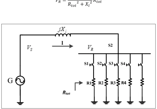
Consider a simple 2-bus system of Figure 3.1. In this figure, bus 1 is the generator bus (PV) and bus 2 is the load bus (PQ). For the sake of simplicity, the load is assumed to be purely resistive. As can be seen in the figure, several loads have been connected to bus 2 in parallel. According to Figure 3.1:
=( ) (3.1)
Where:
: phasor voltage of Bus 2 : phasor voltage of Bus 1
: line reactance
The active power delivered to Bus 2 is
= | | (3.2)
: active power delivered to Bus 2 | |: voltage magnitude of Bus 2
Substituting equation (3.1) in (3.2) gives:
= | | + (3.3) S1 S2 S3 S4 R1 R2 R3 S2 I
G
R4Figure 3.1 Simple 2-Bus system
Suppose that is controlled to remain constant. As the demand is increased by switching on S1, S2, S3, S4 and S5 consecutively, is consequently decreased. As is decreased, the delivered active power to bus 2 increases. In other words, the delivered power to bus 2 is
inversely proportional to the value of . This relationship between the delivered active power and the load impedance is as expected. So, as far as decreasing results in increasing the delivered active power, the network is operating under normal conditions. The relationship between the delivered active power to bus 2 and is not always inversely proportional – rather, there is a specific value of behind which, the relationship between those two parameters becomes directly proportional. Figure 7 illustrates PV curve of Bus 2. In this figure: = | = | || = | || || = | || || || || = | || || || = |
is the value of resistant for which maximum power is delivered to Bus 2. represents the maximum loadability limit of Bus 2. To obtain the value of , one must obtain the derivative of with respect to . A negative sign of the derivative of with respect to means that there is a positive correlation between them: a decrease in results in an increase in (higher portion of the PV curve). On the contrary, a positive sign of the derivative of with respect to means that there is a negative correlation between and : a decrease in results in a decrease of as well (lower portion of the PV curve).
= | |
+ =
| | −
+ (3.4)
For the higher portion of the PV curve:
For the lower portion of the PV curve:
> 0 → < (3.6)
For the nose point of the PV curve that corresponds to Pcr
= 0 → = = (3.7)
Figure3.2 PV curve for bus 2
When the equilibrium point of a load is at the higher portion of the PV curve (equilibrium points A, B and C), injection of reactive power would increase the voltage magnitude. On the contrary, when the equilibrium point of a load is at the lower portion of the PV curve (equilibrium points D and E), injection of reactive power would decrease the voltage magnitude (Lagace 2012). When the equilibrium point of a load is at the nose point of the PV
V P 0 dV dQ > 0 dV dQ < 1 P P2 P3 P4 Pcr
curve (equilibrium point F), injection of reactive power would not result in any variation in the voltage magnitude ( = 0). The nose point is considered to be the point of voltage collapse or the point of maximum loadability. The equilibrium points at the higher portion of the PV curve are voltage controllable, and the equilibrium points at the lower portion of the PV are voltage uncontrollable. Those equilibrium points belong to the lower portion of the PV curve, and are voltage unstable because any corrective action of the voltage control equipment has a negative corrective effect on them.
Diagnosing whether or not the system is operating under a voltage stable condition in order to adopt appropriate control strategies, is very important. The onset of a voltage instability is not always accompanied by a significant voltage drop. However, it could eventually cause a voltage collapse in the entire power system. Even if the voltages of the unstable buses (due to voltage uncontrollability) are viable, treating them the same as the stable buses would lead to worsening the condition of voltage stability of the system. This is due to the fact that injection of reactive power at unstable buses would decrease their voltages.
3.2 Generalization to n-bus system
According to the circuit theory, any arbitrary network composed of n buses can be represented by a voltage source (Vth) and an impedance (Zth). If in the two-bus system, we
replace generator of bus 1 by Vth and also replace line impedance by Zth, all the conclusions
driven for the two-bus system will remain valid. This means, for| |> | |, the equilibrium point is on the higher portion of the PV curve and thus the system is voltage stable. On the contrary, for| |< | | the equilibrium point is on the lower portion of the PV curve and thus the system is voltage unstable. Maximum active power deliverable to any specific bus can be easily calculated, provided that the magnitude of Zth is known. Calculating Zth is not
complicated for the linear networks. For the linear networks Vth of each bus is equal to the
no-load voltage of the same bus, and Zth seen from each bus is computed by dividing the
= (3.8)
Where is the no-load voltage of bus i and is the short circuit current of bus i. It is to be noted that in linear networks for all buses Vnl=Vth.
Calculating Zth for power systems with nonlinear loads and elements is complicated. In the
linear electrical circuits, Zth seen from each node is its corresponding diagonal element of Z
matrix. For example, in a 3 bus circuit the Thevenin impedance seen from the bus 3 is the last diagonal element of its Impedance matrix. It is to be noted that Zth obtained from the Z
matrix includes impedance of the bus where Zth has been obtained, thus the exact Zth seen
from bus ith is calculated as follow:
∗ + = → = + ∗ → = ∗ − (3.9) Where:
is Zth seen from bus ith
is the diagonal element of Z matrix corresponding to bus ith
is the load’s apparent impedance and is calculated from the following equation:
= ∗∗ (3.10)
Where V, ∗ and ∗ are complex numbers and represent voltage, voltage conjugate and apparent power conjugate of ith bus respectively.
Zth obtained from this method is utilized later on in this thesis to estimate maximum
deliverable active power to all the load buses of a power system. As it is mentioned earlier, this method to obtain Zth is valid for linear electrical circuits. Thus, since power systems are a
nonlinear circuit, another approach is required to calculate Zth. In this thesis, a Perturbation &
CHAPTER 4
PROPOSED VOLTAGE STABILITY ASSESSMENT TECHNIQUE
In this chapter, the proposed VSL index is presented. First, the P&O algorithm is employed to obtain the maximum loadability of each bus. The voltage controllability of each bus is then examined using a V-Q sensitivity analysis.
4.1 Maximum loadability tracking
The P&O algorithm is the most popular approach to track the maximum power point in photovoltaic systems. It operates by periodically perturbing (i.e. incrementing or decrementing) the array terminal voltage and comparing the PV output power with that of the previous perturbation cycle. If the power is increasing, the perturbation will continue in the same direction in the next cycle, otherwise the perturbation direction will be reversed (Hussein, Muta et al. 1995).
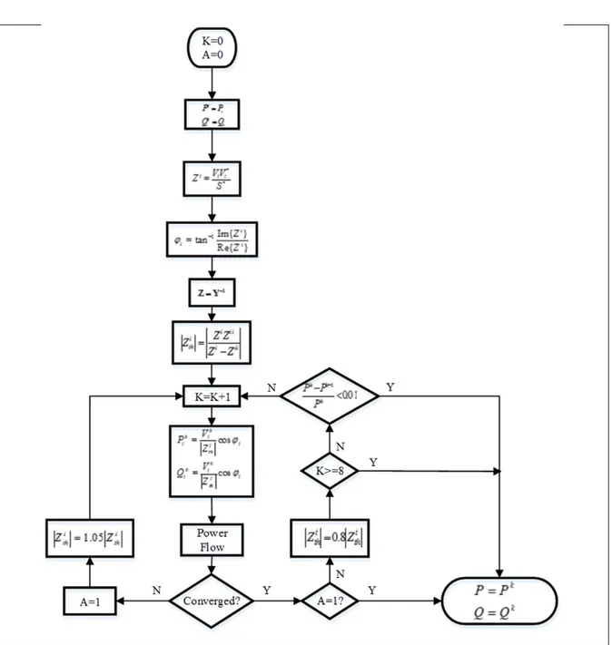
In this thesis the P & O algorithm is used to obtain maximum loadability of all the load buses in a power system. As it was discussed in chapter 3, maximum loadability of any bus is reached when the magnitude of its apparent impedance is equal to the magnitude of the Thevenin impedance seen from the same bus.
Figure 4.1 P & O algorithm to find the maximum deliverable power to bus i 4.2 Detection of Loss of the Voltage Controllability
All voltage control systems (transformer taps, SVCs, shunt capacitors, generators, etc…) assume that injection of reactive power (Q) would increase Voltage magnitude (V). If this assumption is wrong, then the control systems would behave incorrectly by having the opposite effect on the voltage magnitude. QV relationship determines the sensitivity and variation of the bus voltages with respect to the reactive power injections or absorptions. “A
system is voltage stable if Q sensitivity is positive for every bus, and voltage unstable if V-Q sensitivity is negative for at least one bus”(Gao, Morison et al. 1992). In other words, if the voltage of a bus is diminished following an injection of reactive power to that bus, one can conclude that the bus is voltage uncontrollable and hence voltage unstable. Therefore, if the voltage profile of the power system followed by an injection of reactive power to every bus, one by one, is predicted and compared with the current voltage profile of the same bus, the voltage stability condition of each bus is revealed. In order to be more clarified, suppose that a fictitious capacitor is connected to all the buses of the power system; at a moment of time all the fictitious capacitors are off except the fictitious capacitor located at the ith bus. If the voltage variation of the ith bus is positive, one can conclude that the bus is voltage stable. Otherwise, the bus is voltage unstable. Therefore, if we can predict the reaction of the voltage of each bus with respect to injection of reactive power to the bus, then we can identify whether or not the bus is voltage stable.
The Jacobian matrix is employed in Newton-Raphson method to solve power flow problems. At each iteration of the Newton-Raphson method, voltage and angle variations obtained from the previous iteration are used to calculate the active and reactive power variations. The Jacobian matrix relates the angle and voltage variations to the active and reactive power variations. Therefore, using the inverse of the Jacobian matrix, angle and voltage variations due to a slight injection of reactive power can be predicted.
The elements of the Jacobian matrix are calculated from the solved power flow. If the sign of the voltage magnitude variation of the bus corresponding to a positive reactive power variation is negative, one can conclude that the bus is operating in an unstable equilibrium point.
The relationship between the Jacobian matrix, the net injected active and reactive power variation and the voltage magnitude and angle variation is as follows:
2 2 2 2 2 2 2 2 2 2 2 2 2 2 2 2 2 2 2 2 2 n n n n n n n n n n n n m m m m n m n P P P P V V P P P P P P V V Q V Q Q Q Q V V V Q Q Q Q Q V V θ θ θ θ θ θ θ θ θ θ ∂ ∂ ∂ ∂ ∂ ∂ ∂ ∂ Δ Δ ∂ ∂ ∂ ∂ Δ ∂ ∂ ∂ ∂ Δ Δ = ∂ ∂ ∂ ∂ Δ ∂ ∂ ∂ ∂ Δ Δ ∂ ∂ ∂ ∂ ∂ ∂ ∂ ∂ (4.3) Where:
∆ ,…,∆ = variation in the ith bus active power
∆ ,…,∆ = variation in the ith bus reactive power ∆ ,… ,∆ = variation in the ith bus voltage angle
∆ ,…,∆ = variation in the ith bus voltage magnitude
=number of the network buses = number of load buses
Rewriting equation (4.3) in terms of ∆ and ∆ gives: 2 2 1 2 2 n n n m P P J Q V V Q θ θ − Δ Δ Δ Δ = Δ Δ Δ Δ (4.4) Where:
J-1 = inverse of the Jacobian matrix. Equation (4.4) can be rewritten as follow:
11 12 21 22 A A P V A A Q θ Δ Δ = Δ Δ (4.5)
From the equation (4.5), one can obviously conclude that if a particular amount of reactive power is injected at every bus of the network, the voltage of the same bus is varied along the sign of the corresponding diagonal element of A22. In other words, negative signs of the diagonal elements of A22 correspond to voltage unstable buses of the network.
4.3 Proposed VSL index
An algorithm to track maximum loadability of every bus in power systems was proposed in the second section of this chapter. Additionally, an approach to find the voltage uncontrollable buses was proposed in the third section of this chapter. Now, we use the results of the two previous sections to propose a novel index for evaluating stability condition of the power systems.
In a power system with n load bus, the VSL index of the ith bus is obtained from the following equation:
= ( ) − (4.6)
Where:
is the maximum power deliverable to bus i is the current active power of bus i
is the maximum of ( = 1,2, . . )
( ) is the sign of the iith element of the sub matrix in relationship (4.5)
The VSL indices lie between -1 and 1. The bus having a VSL index of 1 has the best stability condition and the bus having a VSL index of -1 implies the worst stability condition. As the VSL index of a specific bus decreases from 1 to 0, the corresponding bus becomes more vulnerable to voltage collapse. When the injected power to a bus is equal to its maximum deliverable power, the numerator of the equation 4.6 becomes zero. Therefore, the VSL index of 0 implies to the nose point of PV curve.
CHAPTER 5
SIMULATION RESULTS AND DISCUSSION
In this chapter, results of applying the VSL technique to the case studies are presented. The results are then compared to those of obtained from L-index.
5.1 Simulation results
5.1.1 Case 1: IEEE 118-Bus system
Maximum loadability limit of all the load buses of IEEE 118-Bus system were obtained by the P&O algorithm. It was found that bus 68 has the maximum loadability limit, and its amount is 38.576 pu (Sb=100MVA). Bus 21 has the minimum loadability limit. Its amount is
1.967 pu.
The three weakest and three strongest buses of the IEEE 118-Bus system are illustrated in tables 5.1 and 5.2 respectively.
Table 5.1 The three weakest buses of IEEE 118-Bus system
Bus number Pi (pu) Qi (pu) Pmi (pu) Qmi (pu) VSL
117 0.2 0.08 2.001 0.799 0.047
21 0.14 0.08 1.967 1.124 0.048
44 0.16 0.08 2.038 1.018 0.048
To validate the results, we chose two buses from each table and plotted the PV curves as well as the VSL index with respect to the variation in injected active power for those buses.
To validate the results, we chose two buses from each table and plotted the PV curves as well as the VSL index with respect to the variation in injected active power for those buses.
As it can be seen in Figure 5.1 as delivered active power to bus 117 is increased from 0.2 pu to about 2 pu which is the nose point of the PV curve, the VSL decreases from 0.047 to 0. It is clear that a VSL of zero corresponds to the nose point of the PV curve. As soon as the equilibrium point reaches the voltage unstable region – i.e the lower portion of the PV curve – the VSL becomes negative. As the load gets heavier, the injected active power at bus 117 decreases and at the same time, the magnitude of the VSL increases but with a negative sign (Figure 5.2). As the VSL moves from 0 to -1, the voltage stability worsens.
Figure 5.3 illustrates the PV curve for bus 21. According to Figure 5.3, increasing the active power delivered to bus 21 from 0.14 pu to 1.967 pu, results in decreasing its VSL index from 0.048 to 0. Moving the operating point from the upper portion of the PV curve to the lower portion is concurrent to changing the sign of the VSL index from positive to negative (Figure 5.4).
Table 5.2 The three strongest buses of IEEE 118-Bus system
Bus number Pi (pu) Qi (pu) Pmi (pu) Qmi (pu) VSL
68 0 0 38.376 0 1
81 0 0 31.589 0 0.824
64 0 0 27.430 0 0.715
According to the VSL indices of the load buses of the IEEE 118-Bus system, bus 68 is the strongest bus of the system. Figures 5.5 and 5.6 illustrate the PV and the VSL-Active Power curves for bus 68 respectively.
Figure 5.1 PV curve for bus 117
Figure 5.3 PV curve for bus 21
Figure 5.4 P-VSL curve for bus 21
Based on the obtained results from the proposed technique, bus 81 is the second strongest bus of the network. As the load connected to this bus gets heavier, the VSL index of bus 81 gets
smaller and becomes 0 at the nose point of the PV curve. Further increase in the demand, results in decreasing the active power delivered to bus 81 as well as decreasing the value of the VSL index. This situation is illustrated in figures 6.7 and 6.8.
Figure 5.5 PV curve for bus 68
Figure 5.7 PV curve for bus 81
Figure 5.8 P-VSL curve for bus 81
Based on the obtained results from the proposed technique, bus 81 is the second strongest bus of the network. As the bus load gets heavier, the VSL index of bus 81 gets smaller and becomes 0 at the nose point of the PV curve. Further increase in the demand, results in
decreasing the active power delivered to bus 81 as well as decreasing the value of the VSL index. This situation is illustrated in figures 5.7 and 5.8.
5.1.2 Case 2 Hydro-Quebec network
VSL indices were calculated for all the load buses. The three weakest and strongest buses of the Hydro-Quebec network are tabulated in tables 5.3 and 5.4 respectively.
Table 5.3 The three weakest buses of Hydro-Quebec network
Bus number Pi (pu) Qi (pu) Pmi (pu) Qmi (pu) VSL
638 0.646 0.148 0.952 0.218 0.011
559 0.056 0.011 0.453 0.0848 0.014
634 0 0 0.389 0 0.014
Table 5.4 The three strongest buses of Hydro-Quebec network
Bus number Pi (pu) Qi (pu) Pmi (pu) Qmi (pu) VSL
141 0 0 27.111 0 1
261 0 0 24.315 0 0.934
408 2.84 0.37 24.005 3.336 0.840
Based on the results obtained, bus 638 is the weakest bus and bus 141 is the strongest bus of the network. The active power consumption of the load located at bus 638 is 0.646 pu. According to Table 5.3, if the demand at bus 638 is increased to about 0.96 pu, the Hydro-Quebec system will become unstable because the maximum loadability limit of bus 638 is less than 0.96 pu. The PV and the VSL-Active Power Curves for bus 638 are depicted in
figures 5.9 and 5.10 respectively. The VSL index for this bus at the given load condition is 0.011. This small value for the VSL index implies a very small loadability margin for bus 638.
According to the VSL indices obtained for Hydro-Quebec network, bus 634 is the third weakest bus of the network. This bus reaches its maximum loadability limit at P=0.389 pu. Figure 5.11 illustrate the PV curve of bus 634. It can be seen from Figure 5.12 that as the operating point moves on the PV curve toward the nose point, the VSL index of this bus decreases from 0.014 to 0. The VSL index becomes negative when the operating point moves to the lower portion of the PV curve.
Based on the results obtained from the VSL indices, bus 141 is the strongest bus of the Hydro-Quebec network. The maximum loadability limit of this bus is 27.111 pu. The voltage instability phenomenon is likely to initiate from bus 141 because of this large loadability margin of this bus. The PV and VSL-Active Power Curves for bus 638 are depicted in figures 5.13 and 5.14 respectively.
Figure 5.9 PV curve for bus 638
Figure 5.10 P-VSL curve for bus 638
The second strongest bus of the Hydro-Quebec network is bus 261 whose maximum loadability limit is 24.315 pu. The PV and VSL-Active Power Curves for bus 261 are depicted in figures 5.15 and 5.16 respectively.
Figure 5.11 PV curve for bus 634
Figure 5.13 PV curve for bus 141
Figure 5.15 PV curve for bus 261
5.1.3 Case 3: 2736-Bus system
The VSL indices were computed for all the load buses. The results for three weakest and three strongest buses of this test case are tabulated in tables 5.5 and 5.6 respectively.
Table 5.5 The three weakest buses of 2736-Bus system
Bus number Pi (pu) Qi (pu) Pmi (pu) Qmi (pu) VSL
2164 0.063 0.743 0.191 23.312 0.002
506 0.032 0.010 0.561 0.172 0.006
2166 0.010 0.004 0.761 0.259 0.009
Table 5.6 The three strongest buses of 2736-Bus system
Bus number Pi (pu) Qi (pu) Pmi (pu) Qmi (pu) VSL
92 0 0 54.928 0 1
90 0 0 48.892 0 0.890
89 0 0 48.891 0 0.890
Based on the results obtained from VSL index analysis, the weakest bus of this system is bus 2164 which has the maximum loadability of 0.191 pu. Buses 506 and 2166 are the two next weakest buses of 2376-Bus system with the maximum loadabilities of 0.561 pu and 0.761 pu respectively.
Figures 5.17 and 5.18 demonstrate the PV and VSL-Active Power curves for bus 2164. It can clearly be seen that the delivered active power corresponding to the nose point of the PV
curve coincide to the point where the value of the VSL index becomes zero. The same scenario applies to bus 506 which is the second weakest bus of this system (figures 5.19 and 5.20).
Figure 5.17 PV curve for bus 2164
Figure 5.19 PV curve for bus 506
Bus 92 has the largest stability margin and therefore it is considered as the strongest bus of this system. Figures 5.21and 5.22 demonstrate the PV and VSL-Active Power curves for bus 92.
Figure 5.21 PV curve for bus 92