HAL Id: hal-01168116
https://hal.archives-ouvertes.fr/hal-01168116
Submitted on 13 Nov 2019
HAL is a multi-disciplinary open access
archive for the deposit and dissemination of
sci-entific research documents, whether they are
pub-lished or not. The documents may come from
teaching and research institutions in France or
abroad, or from public or private research centers.
L’archive ouverte pluridisciplinaire HAL, est
destinée au dépôt et à la diffusion de documents
scientifiques de niveau recherche, publiés ou non,
émanant des établissements d’enseignement et de
recherche français ou étrangers, des laboratoires
publics ou privés.
GraphBPT: An Efficient Hierarchical Data Structure for
Image Representation and Probabilistic Inference
Abdullah Al-Dujaili, François Merciol, Sébastien Lefèvre
To cite this version:
Abdullah Al-Dujaili, François Merciol, Sébastien Lefèvre. GraphBPT: An Efficient Hierarchical Data
Structure for Image Representation and Probabilistic Inference. International Symposium on
Math-ematical Morphology, 2015, Reykjavik, Iceland. pp.301-312, �10.1007/978-3-319-18720-4_26�.
�hal-01168116�
GraphBPT: An Efficient Hierarchical Data
Structure for Image Representation and
Probabilistic Inference
Abdullah Al-Dujaili1,2, Fran¸cois Merciol1, and S´ebastien Lef`evre1
1
Univ. Bretagne-Sud, IRISA, Vannes, France {francois.merciol,sebastien.lefevre}@irisa.fr
2 Nanyang Technological University, School of Computer Engineering, Singapore
Abstract. This paper presents GraphBPT, a tool for hierarchical rep-resentation of images based on binary partition trees. It relies on a new BPT construction algorithm that have interesting tuning properties. Be-sides, access to image pixels from the tree is achieved efficiently with data compression techniques, and a textual representation of BPT is also pro-vided for interoperability. Finally, we illustrate how the proposed tool takes benefit from probabilistic inference techniques by empowering the BPT with its equivalent factor graph. The relevance of GraphBPT is illustrated in the context of image segmentation.
Keywords: image processing, hierarchical segmentation, binary parti-tion tree, compression, probabilistic inference
1
Introduction
A strong interest in the recent decades has been developed towards realizing ma-chines that can perceive and understand their surroundings. However, computer vision is still facing a lot of challenges even with high-performance computing systems. One of these challenges is how to deal with the input of these machines. Typically, the input to computer vision is of images in their pixel-based rectan-gular representation, whereas the output is associated with actions or decisions. Clearly, what kind of output or performance is desired from such a system im-poses a set of constraints on the visual data representation. A representation for a storage-efficient system is not the same as for high-accuracy systems.
In these early approaches for analyzing visual data, pixels were treated inde-pendently [1]. This proved to be successful for a while but the increase in image resolution due to the advancing sensors technology created the need for a model that considers spatial relationships. This led to context-based models such as superpixels, edge-based, and segmentation-based representations, that brought up the object-based paradigm [2]. Although such models show an advantage in several applications [3], it still experienced uncertainty in defining what a con-text is due to factors like scale, concon-text inter- and intra-variance. Consequently,
the concept of hierarchical representation was adopted and it has proven useful in analyzing images [4–6]. The acyclic nature of some of these representations makes many of the growing machine-learning techniques exact and efficient. For instance, the belief propagation algorithm for probabilistic inference is exact on tree-graphical models [7].
In this paper, we focus on the binary partition trees (BPTs), a special case of hierarchical representations that allows for greater flexibility than many other morphological trees. We elaborate on this representation and introduce three complementary contributions to the state-of-the-art:
1. An efficient implementation of BPT construction algorithm. The implemen-tation offers a flexible framework to specify and control the way a BPT is built. The code is freely available3under LGPL license4.
2. A textual representation of the BPT which makes it portable across different programming environments and platforms.
3. A demonstration of empowering BPTs with probabilistic inference.
These contributions aim to support the dissemination of the BPT (and more generally hierarchical representations) to solve computer vision problems.
The paper organization is as follows. We first recall in Sec. 2 the concept of BPT and introduce in Sec. 3 an efficient algorithm for its computation. We then propose in Sec. 4 a compact and portable representation of BPTs through textual files, with efficient access to image data. Sec. 5 presents how BPT can be combined with the framework of probabilistic inference, with an illustrative application in image segmentation. The last section is dedicated to conclusion and future directions.
2
Binary Partition Tree (BPT)
There exist several hierarchical representations that come with useful properties, e.g. min- and max-trees [8], component trees [9], or trees of shapes [10] that all aim to extract regional extrema of the image. However, such regions sometimes do not correspond to objects in the scene. On the other hand, the nodes of a binary partition tree (BPT) are potential candidates for objects as BPT is able to couple image regions based on their similarities.
BPT was introduced in [11, 12] as a structured representation of the regions that can be obtained from an initial partition using binary mergings. In other words, it is an agglomerative hierarchical clustering of image pixels (see Figs. 3, 4, and 5 for an illustration with a color image, its associated tree, and the nested partitions, respectively). Image filtering, segmentation, object detection and recognition based on BPT were demonstrated e.g. in [12–16].
The basic framework of constructing a BPT is simple and straightforward: starting with the image pixels as the initial regions, a BPT is constructed by
3
http://www-obelix.irisa.fr/software
4
successively merging the most similar pairs of regions until all regions are merged into a single region [17]. The process is governed by the following factors [11]:
– Region Model defines how each region is represented based on its charac-teristics, e.g. color, shape, texture, etc.
– Merging Criterion defines a score of merging two regions. It is a function of their region model.
– Merging Order defines the rules to guide the merging process based on merging criterion.
There is no unique choice for these various parameters. However, a commonly adopted strategy is to represent each region by its average color in a given color space, and to first merge two regions that either have models similar one to each other, or similar to the model of the region built from their possible union [14]. Furthermore, Vilaplana et al. [14] also explore how to take into account edge and contrast information in the merging process through advanced merging cri-teria. Let us note that, similarly to the underlying BPT model, the methodology proposed in this paper is generic, i.e. it can be apply to various region models and merging criteria.
3
BPT Construction
Based on the strategy proposed for building a BPT in [17], Valero et al. [16] described an algorithm for constructing BPTs and presented a detailed analysis on its complexity. For an (N = m ∗ n)-pixel image and assuming 4-connectivity, the complexity can be expressed as the following:
OBP T(N ) = N ∗ Oleaf+ (4 ∗ N ) ∗ (Oedge+ Oinsert) + (N − 1) ∗ Omerge (1)
where Oleaf, Oedge, Oinsert = O(log2N ) are the complexity costs of building a
leaf node, building an edge between two nodes, inserting an edge into the priority queue, respectively. Omerge = Oparent+ a ∗ (Oedge+ Oinsert) + b ∗ Opop is the
complexity of merging two nodes; with Oparent being the cost for constructing
their parent node, and Opop being the cost of poping an edge off the priority
queue. Scale factors a and b correspond respectively to the number of parent node’s neighbors and the number of two nodes’ neighbors. Here, we describe an optimized algorithm that lowers some of the terms in Eq. (1).
3.1 Proposed Algorithm
First, the leaf nodes are computed from the image N pixels. Their edges are also built based on the 4-connectivity scheme. Each edge is built once, so the term (4 ∗ N ) becomes (2 ∗ N − m − n). Moreover, instead of inserting all the edges for a node, we insert only the most light edge (corresponding to the most similar neighboring pixels) into the queue; all other edges are irrelevant for the node of interest. Nevertheless, if it gets merged into a new node, then all of
Algorithm 1: Proposed Algorithm for BPT Construction Input : An image I of N pixels
Variables: Min-Priority Queue P Q,
A set of nodes V representing the binary partition tree nodes, A set of edges E connecting neighboring nodes
Output : Binary partition tree of the image BP T
1 foreach pixel p of the image I do
2 u ←BuildLeafNode (p)
3 BP T ← UpdateBPT (u)
4 foreach neighboring pixel q of p do
5 v ← leaf node of q 6 Euv←UpdateNeighborhoodEdges (u,v) 7 P Q.insert(Euv.smallestEdge) 8 for i ← 1 to N − 1 do 9 do 10 e ← P Q.getHighestPriority()
11 while(e.nodes() have no parents)
12 u, v ← e.nodes()
13 w ← BuildParentNode (u, v)
14 BP T ← UpdateBPT (w)
15 Ew←UpdateNeighborhoodEdges (w, neighbors of u, neighbors of v)
16 P Q.insert(Ew.smallestEdge)
17 return BP T
its neighbours are going to be considered even those whose connecting edges are not in the queue. This considerably reduces the priority queue size as only one insert per node is carried out, whilst the image support is fully considered. Consequently, the number of insertions and pops is decreased. Nodes are merged successively in N − 1 steps. In each of the merging steps, an edge is taken off the queue, one edge (the most light one) is inserted due to the new neighborhood formed; while edges of the merged nodes in the queue are invalidated. We do not bother about removing the invalidated edges from the priority queue. Instead, whenever a merging step is done, we pop edges from the priority queue and merge on the first valid popped edge. This on average, brings the factor b down to a b0. At the N − 1 step, the BPT root is computed and the BPT construction is complete. The optimized algorithm is listed in Alg. 1.
3.2 Efficiency evaluation
The new algorithm comes with the following complexity:
OBP T0(N ) = N ∗Oleaf+(2∗N −m−n)∗Oedge+N ∗Oinsert+(N −1)∗Omerge0 (2)
with
Table 1: Performance statistics for a subset of MSRA images (120, 000 pixels) Performance CPU time
statistics (in seconds) Minimum 1.499 Maximum 66.277 Standard Deviation 3.788
Mean 2.534
Mode 1.663
Let aaverage and b0average be the average estimation of a and b0, respectively.
With Opop= O(log2(N )) and Oedgebeing a constant operation, the complexity
can be approximated as:
OaverageBP T0 (N ) ≈ O(N ∗ aaverage) + O(N ∗ b0average∗ log2(N )). (4)
A close look on b0 shows that it can have an average estimation of ≈ 1 because in the beginning the priority queue has N edges and each of the N − 1 merging steps adds a single edge and pops one valid edge. Hence the average number of popped invalid edges b0averageis 2N −1N −1 − 1 ≈ 1. Similar analysis can be conducted on a, leading to an average number being a fraction of N , with a peak of 23N in the worst case (i.e. a thin elongated region).
Besides theoretical analysis, we also evaluated efficiency through runtime measurement. Previous implementations of BPT in the literature reported an execution time of 1.5 seconds for a 25, 344-pixel image on a 200 MHz processor [11] and 1.03 seconds on a 1.87 GHz processor for the same image size [14]. Alg. 1 (coded in Java) reported an execution time of 0.282 seconds on a 2.2 GHz for the same image size.
A further analysis was conducted on MSRA’s 5, 000 images [18]. We ran our code with no tuning of BPT parameters and choosing the spectral similarity as the region model. The execution time varies from 0.6 seconds for a 36, 630-pixel color image to 3.8 minutes for a 154, 400-pixel color image. Although the execu-tion time is greatly affected by the number of pixels N , it is as well affected by the image content. Indeed, image content determines the weights of nodes edges which consequently affect the performance of both priority queue operations and image regions compression. Table 1 shows the execution time statistics for 1238 color images of 120, 000 pixels using a 2.2 GHz processor. As a future work, we plan to study extensively the effects of the similarity measures and provide a benchmark for comparing various implementations of BPT.
3.3 BPT tuning
As already indicated, the BPT model is attractive due to its flexibility. We keep such property in our tool by providing a set of tunable parameters to fit the ap-plication needs (e.g. in object detection, regions of compact geometry are usually more preferred over others which might not be the case for a segmentation-based
Table 2: BPT construction parameters
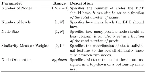
Parameter Range Description
Number of Nodes [1, 2N − 1] Specifies the number of nodes the BPT should have. It can also be set as a fraction of the total number of nodes.
Number of levels [1, N ] Specifies how many levels the BPT should have.
Node Size [1, N ] Specifies how many pixels a node should at least contain. It can also be set as a fraction of the total number of pixels.
Similarity Measure Weights [0, 1]k Specifies the contribution of the k
individ-ual features to the overall similarity mea-sure between two nodes.
Node Orientation up, down Specifies whether the nodes levels are as-signed in a top-down or a bottom-up man-ner.
application). Currently, these parameters can be set from the source files. As a future work, we intend to add a friendly interface to the tool for setting them. Table 2 lists these parameters. Some of them are related and might override each other. For instance, the number of nodes and levels for a tree are quite related (a binary tree of l levels, has at most 2l− 1 nodes). Controlling BPT’s
number of nodes, number of levels, and their sizes helps in bringing images of different scale or size to a normalized representation under their BPTs. The tree construction relies on a similarity between nodes, that is computed here as a linear combination of k similarity measures. Such measures as well as their contribution to the overall similarity measure can be tuned as well. Let us note that we consider in this paper three measures dealing respectively with color, spatial, and geometric information. As BPTs could have irregular structure (e.g. leaf nodes can have different distances from the root), we provide a parameter, node orientation, that assigns the level of each node based on its distance from either the root level (level 1) or the leaf nodes level (specified by the parameter, number of levels). In other words, each node can be assigned to a level either in a top-down or a bottom-up order.
4
BPT Indexing and Management
4.1 Textual Representation
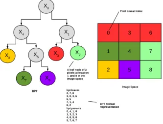
To make our BPT implementation portable and readable across different pro-gramming environments and platforms, we worked out a compact textual repre-sentation of the BPT. The labels: 0, . . . , N − 1 are assigned to the nodes of an N -BPT in a depth-first order from right to left as shown in Fig. 1.
1 4 X4 X1 X0 X3 X2 X8 X5 X7 X6 6 0 3 7 8 2 5
Pixel Linear Index
BPT Image Space bpt.leaves 2, 7, 8 3, 0, 3, 6 6, 5 7, 1, 4 8, 2 bpt.parents 0, 4, 1, 8 1, 3, 2, 3 4, 8, 5, 8 5, 7, 6, 7 A leaf node of 2 pixels at location 7, and 8 in the image space BPT Textual Representation
Fig. 1: BPT textual representation
Each leaf node l is represented with a single line of comma-separated values (csv) as the following: [Al, Bl] where Al is the node label, and Bl is the set of
node’s pixels linear indices. On the other hand, each parent node p is represented by the line: [Cp, Dp, Ep, Fp] where Cp is the node label, Dp, Ep are the children
nodes labels in a descending order, and Fpis the greatest label among descendant
nodes labels. Such a textual representation allows to build BPTs in a top-down approach directly. Besides, indexing p’s image region is nothing but the pixels union of leaf nodes whose labels Alintersect with the interval [Ep, Fp].
As each node is represented with a csv line, it is easy to add any other feature/attribute to its textual representation. For instance, the number of de-scendant nodes can be appended for each node to help in drawing the tree. Our tool automatically produces two text files named as bpt.leaves and bpt.parents which can be read readily to retrieve the BPT structure. Along with the tool, we have provided MATLAB functions for accessing these files and producing the BPT structure in a MATLAB environment.
4.2 Region Indexing
Given a node, it is sometimes needed to access the corresponding region in the image space. Usually, the leaf nodes would have the direct access to the image pixels. As a result, graph traversal is the technique commonly used to traverse from a node of interest to its descendant leaf nodes, and hence accessing the corresponding image region. To avoid traversing the tree, and provide a direct access to a node’s image region, a bounding box is created for each node that
covers all the pixels included in the corresponding image region, as well as some neighboring pixels (i.e. pixels that belong to the bounding box but do not belong to the node of interest). This provides two advantages:
1. It makes BPT more adaptable to grid/window-based computer vision models and paradigms such as kernel descriptors [19] and convolutional networks [4]. 2. It provides a constant time operation for accessing a relaxed representation
(bounding box) of a specific node.
Nevertheless, to retrieve the node’s exact image region, the bounding box can be provided with a bitmap whose bits correspond to the pixels within the bounding box. A bit is set to 1 if the corresponding pixel belongs to the node, or 0 other-wise. The additional memory storage incurred by these bitmaps can significantly be reduced by compressing them using a suitable compression technique. The tool currently uses run-length encoding (RLE) to compress the BPT’s bitmaps. This adds to the complexity of Oparent in Eq. (3) a term that is linear in the
number of pixels in newly-formed node.
5
Probabilistic Graphical Model for BPT
Some of the problems in the domain of computer vision such as object detection and recognition are naturally ill-posed in a way that it is very difficult to deter-mine with absolute certainty their exact solutions. In these settings, probabilistic graphical models become very handy in not only providing a single solution but a probability distribution over all feasible solutions [20]. Therefore, instead of the conventional methods that analyse each node as a separate entity for ex-ample in object detection and recognition problems [13], treating the BPT as an entire structure by encoding the relationships between its nodes is elegantly done using a probabilistic graphical model. Here, we focus on representing BPTs with a discrete factor graph with a conditional distribution. The reader is re-ferred to [20] for an introduction to these models. The practical interest of such a connection between morphological representations and probabilistic inference will be illustrated in the context of image segmentation.
5.1 Inducing a BPT’s factor graph
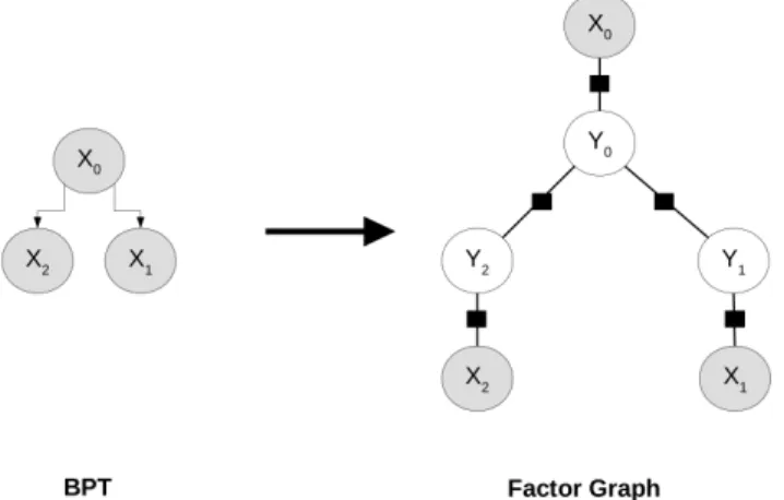
A BPT can be defined as the tuple (X, E) where X is the set of measure-ments/observations nodes (color, shape, or other features) that correspond to the BPT nodes and E is the set of edges connecting the nodes and hence X. X can be considered as the set of input variables that are always available. On the other side, an output variable is provided for each node and collectively denoted as Y . Their values represent the solution to the problem of interest. For instance, in object detection, we can have a binary variable per node to denote whether it corresponds to a sought object or not. The factor graph captures the interaction among these variables by introducing a set of factor nodes F . These factors can
be seen as potential functions that assign scores to the output variables assign-ments and are application-dependent. Let V = X ∪ Y , then the factor graph is the tuple (V, F , E ) where E ⊆ V × F . Figure 2 shows how a factor graph is induced from a BPT.
Fig. 2: Inducing a factor graph from a 3-BPT
5.2 Probabilistic Inference on BPT
Once the factor graph is built, probabilistic inference is a straightforward process. We integrated libDAI [21], a free and open source C++ library for performing probabilistic inference. As the generated factor graph is of a tree structure, inference is efficient and exact. For an output variable domain of L, the inference complexity is of O(|Y ||L|2). We recall that performing an exact inference on a general network is NP-hard [22, 23].
5.3 Application
We demonstrate here how the tool can be used for one of the most common problems in computer vision, namely image segmentation (into foreground and background). Given an image, we would like to segment out the object of interest using BPT. In other words, we are interested in labelling BPT nodes and hence image regions with either foreground and background class. As a first step, the BPT is built from the initial image. Figure 4 shows BPT built for the image in Fig. 3. As we are targeting objects of homogeneous texture, the contribution of color information to the similarity measure is set to be the highest. As already indicated, other sources of information (e.g. edge, spatial, geometric, or com-plex features) could be considered for the similarity measure depending on the application context.
Fig. 3: Input Image 0 1 2 3 4 5 7 8 9 10 6 11 12 13 14 15 16 17 18 19 20 21 22 23 24 25 26 27 28 29 30 31 32 33 35 34 36 37 38 39 40 Fig. 4: BPT
Conversely from previous approaches in analyzing BPTs, we deal with them holistically by performing probabilistic inference on their induced factor graphs. Put it mathematically, a node xi in the BPT X has a label variable yi∈ {0, 1},
and Y = {yi} is the set of X’s nodes label variables. Our goal is to find the
highest probable joint assignment of Y given X:
Y∗= arg max
Y ∈{0,1}|Y |
P (Y |X) (5)
where P (Y |X) is nothing but the normalized product of the BPT’s factor graph factors: P (Y |X) = 1 Z(F ) Y f ∈F :yf∈Y,xf∈X φf(yf; xf) (6)
with Z the normalizing function for a proper probability distribution and φf the
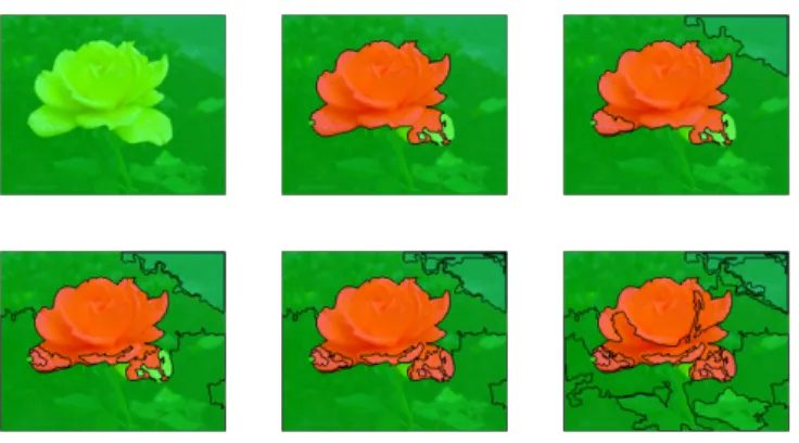
potential function for the factor node f [20]. A crucial aspect of exploiting the power of factor graphs is how carefully factors (potential functions) are designed. These factors can be either hand-crafted or learned using well-established ma-chine learning techniques to suit more complex problems. For the sake of demon-stration, we have designed the factors based on nodes color information. Figure 5 shows the labelling of BPT nodes across its six levels with transparent green assigned to background nodes and transparent red assigned to foreground ones.
6
Conclusion
This paper presented an efficient tool for building and managing binary partition trees as hierarchical representations of images. It relies on a new algorithm that allows for efficient BPT construction, while still offering several control param-eters to guide the construction process. Besides, we also introduced an indexing scheme based on compressed bit maps of the nodes regions. With an additional manageable storage cost, it avoids the recursive graph traversals that is usually needed for accessing all pixels belonging to a BPT node. Furthermore, empower-ing the BPT with probabilistic inference features is made available by inducempower-ing the corresponding factor graph of the BPT. As the induced factor graph is as
Fig. 5: BPT Nodes Labels
well acyclic, probabilistic inferences are exact and efficient. These complemen-tary contributions, gathered in a publicly available tool, support the BPT as a tunable model that can be combined with recent machine learning paradigms to solve various computer vision problems.
We have provided here only a very limited comparison with existing works [11, 14]. In order to better assess the relevance of our findings, we plan now to perform a deeper experimental evaluation of our contributions (both the compu-tational cost of the construction algorithm and the memory cost of the proposed data structure) and to compare them with more recent works, e.g. [24]. Besides, we are considering to apply the proposed probabilistic framework to various problems faced in computer vision, e.g. object recognition or image classifica-tion. To do so, we will also need to explore various similarity measures and their impact on the performance of the resulting BPT model.
References
1. Hussain, M., Chen, D., Cheng, A., Wei, H., Stanley, D.: Change detection from remotely sensed images: From pixel-based to object-based approaches. ISPRS Journal of Photogrammetry and Remote Sensing 80 (2013) 91–106
2. Blaschke, T., Lang, S., Lorup, E., Strobl, J., Zeil, P.: Object-oriented image pro-cessing in an integrated GIS/remote sensing environment and perspectives for en-vironmental applications. Enen-vironmental information for planning, politics and the public 2 (2000) 555–570
3. Walter, V.: Object-based classification of remote sensing data for change detection. ISPRS Journal of Photogrammetry and Remote Sensing 58(3–4) (2004) 225–238 4. Farabet, C., Couprie, C., Najman, L., LeCun, Y.: Learning hierarchical features for
scene labeling. IEEE Transactions on Pattern Analysis and Machine Intelligence 35(8) (2013) 1915–1929
5. Lefvre, S., Chapel, L., Merciol, F.: Hyperspectral image classification from multi-scale description with constrained connectivity and metric learning. Proceedings
of the 6th International Workshop on Hyperspectral Image and Signal Processing: Evolution in Remote Sensing (WHISPERS 2014) (2014)
6. Valero, S., Salembier, P., Chanussot, J.: Hyperspectral image representation and processing with binary partition trees. IEEE Transactions on Image Processing, 22(4) (2013) 1430–1443
7. Koller, D., Friedman, N.: Probabilistic Graphical Models: Principles and Tech-niques - Adaptive Computation and Machine Learning. The MIT Press (2009) 8. Salembier, P., Oliveras, A., Garrido, L.: Antiextensive connected operators for
image and sequence processing. IEEE Transactions on Image Processing 7(4) (1998) 555–570
9. Jones, R.: Component trees for image filtering and segmentation. In: IEEE Work-shop on Nonlinear Signal and Image Processing (NSIP). (1997)
10. Monasse, P., Guichard, F.: Scale-space from a level lines tree. Journal of Visual Communication and Image Representation 11(2) (2000) 224–236
11. Garrido, L., Salembier, P., Garcia, D.: Extensive operators in partition lattices for image sequence analysis. Signal Processing 66(2) (1998) 157–180
12. Salembier, P., Garrido, L.: Binary partition tree as an efficient representation for image processing, segmentation, and information retrieval. IEEE Transactions on Image Processing 9(4) (2000) 561–576
13. Salerno, O., Pard`as, M., Vilaplana, V., Marqu´es, F.: Object recognition based on binary partition trees. In: International Conference on Image Processing. Vol-ume 2., IEEE (2004) 929–932
14. Vilaplana, V., Marques, F., Salembier, P.: Binary partition trees for object detec-tion. IEEE Transactions on Image Processing 17(11) (2008) 2201–2216
15. Gir´o-i Nieto, X.: Part-Based Object Retrieval With Binary Partition Trees. PhD thesis, Universitat Polit`ecnica de Catalunya (UPC) (2012)
16. Valero, S., Salembier, P., Chanussot, J.: Hyperspectral image representation and processing with binary partition trees. Image Processing, IEEE Transactions on 22(4) (2013) 1430–1443
17. Garrido, L.: Hierarchical Region Based Processing of Images and Video Sequences: Application to Filtering, Segmentation and Information Retrieval. PhD thesis, Universitat Polit`ecnica de Catalunya (UPC) (2002)
18. Liu, T., Yuan, Z., Sun, J., Wang, J., Zheng, N., Tang, X., Shum, H.Y.: Learning to detect a salient object. IEEE Transactions on Pattern Analysis and Machine Intelligence 33(2) (2011) 353–367
19. Bo, L., Lai, K., Ren, X., Fox, D.: Object recognition with hierarchical kernel descriptors. In: IEEE Conference on Computer Vision and Pattern Recognition (CVPR), IEEE (2011) 1729–1736
20. Nowozin, S., Lampert, C.H.: Structured learning and prediction in computer vision. Foundations and Trends in Computer Graphics and Vision 6(3–4) (2011) 185–365 21. Mooij, J.M.: libDAI: A free and open source C++ library for discrete approximate inference in graphical models. Journal of Machine Learning Research 11 (August 2010) 2169–2173
22. McAuley, J., Campos, T.d., Csurka, G., Perronnin, F.: Hierarchical image-region labeling via structured learning. In: Proceedings of the British Machine Vision Conference, BMVA Press (2009) 49.1–49.11
23. Cooper, G.F.: The computational complexity of probabilistic inference using bayesian belief networks. Artificial intelligence 42(2) (1990) 393–405
24. Najman, L., Cousty, J., Perret, B.: Playing with kruskal: Algorithms for morpholog-ical trees in edge-weighted graphs. In: International Symposium on Mathematmorpholog-ical Morphology. (2013) 135–146