Maisonnave: Corresponding author. Université Laval, CIRPÉE and PEP network, Canada
helene.maisonnave@ecn.ulaval.ca
Mabugu: Financial and Fiscal Commission, South Africa Chitiga: Human Sciences Research Council, South Africa Robichaud: Université Laval, CIRPÉE and PEP network, Canada
Equal authorship is assigned.
Cahier de recherche/Working Paper 13-10
Analysing Job Creation Effects of Scaling Up Infrastructure Spending
in South Africa
Hélène Maisonnave Ramos Mabugu Margaret Chitiga Véronique Robichaud Mai/May 2013Abstract:
In a first for South Africa, we draw on literature on infrastructure productivity to model dynamic economywide employment impacts of infrastructure investment funded with different fiscal tools. According to the South African investment plan, the policy will affect the stock of infrastructure as well as the stock of capital of some private and public sectors. Increased government deficit financed infrastructure spending improves GDP and reduces unemployment. However, in the long term, the policy reduces investment and it is not sustainable for South Africa to let its deficit grow unabated. Increased investment spending financed by tax increases has contrasting implications on unemployment. In the long run, unemployment decreases for all types of workers under one of the scenarios. In the short run, only elementary occupation workers benefit from a decrease in unemployment; for the rest, unemployment rises. Findings have immediate policy implications in various policy modelling areas.
Keywords: Employment, dynamic CGE model, infrastructure scale up, externalities,
South Africa
2
1 Introduction
The literature on the causes of economic growth5 presents evidence that infrastructure and capital formation are important determinants of economic growth and rising per capita incomes over time. This is a lesson that has been well learned and applied in Asian economies over the last several decades where large public investments have contributed to high economic growth. According to Estache (2007), infrastructure seems to be returning to the agenda of development economists. In South Africa, investment in infrastructure in the years preceding democracy was in general very low. During the era of Growth, Employment and Redistribution (GEAR) from 1996 to 2002, public infrastructure investment fell from 8.1% to 2.6% of gross domestic product (GDP). The emphasis during that time was fiscal discipline more than expenditure increase. It was from the Accelerated and Shared Growth for South Africa (AsgiSA) plan in 2002 that a drive for infrastructure was couched explicitly in policy. Today, the main pillars of government economic policy, the New Growth Path (NGP), the Industrial Policy Action Plan and the National Development Plan (NDP), are anchored in a significant ramping up of current and capital expenditure by the state. The government and state-owned companies plan to spend about R845bn on infrastructure over the next three years, which they expect will contribute significantly to meeting the government job-creation target of 5-million jobs in 2020 (NGP) or 11 million jobs by 2030 (NDP). So much is riding on this state infrastructure spending as the solution to reducing poverty, inequality and unemployment and generating economic growth. The question whether there are economic gains from the provision of higher levels of public spending on capital is fundamental6. If a higher level of capital raises the growth path of the economy then it is justifiable on both equity and efficiency grounds. Whilst no one will argue about the equity issues involved, some will no doubt argue that additional public spending can create efficiency costs. There are a number of possible reasons for this. Firstly, whilst public capital is usually productive, this is by no means the consensus view empirically, and the literature contains a wide variety of estimates of the size of the marginal product of public capital ranging from positive to negative. Even if it is assumed that the marginal product of additional public spending is positive, critics might presumably ask further questions. First, is the effect of such spending permanent or temporary, and if temporary, of what magnitude and after what period of time can one expect positive effects? Government spending on public sector capital may have positive multiplier effects and may, therefore, raise economic activity and thus economic growth. However, once installed will these effects drop to zero? The answer here is not clear. In a Solow - type growth model the effects on growth would be expected to be transitory, positive initially, but zero in the new steady state with a higher level of output. But if public capital raises education and innovation, which might be expected in South Africa, the
5See Aghion and Howitt (2000). 6
3
effects could be permanent and indeed much of the gains could come from spillover effects raising the productivity of private sector capital and labour. Secondly, critics of public spending would presumably argue that even if public capital has a positive effect, its magnitude would need to be compared to the productivity of private sector capital, if inefficient public capital spending is crowding out efficient private sector capital the effects on the economy could be negative. Thirdly, consideration would have to be given to how the public spending is financed. Raising taxes or borrowing could both have negative effects on economic activity which might offset the gains of public sector capital spending.
This paper reflects on the current state and likely future of South African infrastructure investment policy, focusing specifically on government infrastructure spending and how alternative financing arrangements will affect employment, both in the short and longer-term. For these purposes, a recursive dynamic computable general equilibrium (CGE) model with elaborate labour market disaggregation, government budget constraints and alternative funding options for infrastructure scale up is used. The rest of the paper is structured as follows. Section 2 reviews the literature to situate the study, followed by a presentation of the model and data in section 3. Section 4 presents the simulations and implications of introducing alternative infrastructure investment in such a framework. We close the paper with concluding remarks and policy recommendations in section 5.
2 Literature Review
(Neo) classical economics generally assumes that activist fiscal policy is unnecessary to increase employment and production. Government expenditure is generally believed to be consumptive and leading to crowd out of private investment if financed with public debt. Wagner’s law assumes that public expenditure is endogenous and hence cannot be used as a policy lever. Politicians at best should pursue balanced budget strategies. Keynesian economists on the other hand believe that public expenditure is important in determining the level of income as well as its distribution. The market mechanism would not be sufficient to restore full employment. There is a substantial body of empirical literature related to the public expenditure-economic growth nexus (see Moreno-Dodson (2009) for a review of government spending and economic growth studies). An important strand of the literature of direct relevance for this study is the idea that the composition of public expenditures (capital versus current) can have differential impacts on economic growth.
There is an extensive literature, both theoretical and empirical, on the effects of public capital spending on output dating back to Arrow and Kurz (1970) and Aschauer (1989). During the 1980s and 1990s, there was strong academic interest (particularly in the United States of America), on the link between public investment in infrastructure and economic growth. From the outset, it is interesting to note the trend in which this research has followed, from the initial
4
headline estimates of a production elasticity of 0.4 in 1989 to the more modest assessments of 0.1 in 1997. The link between infrastructure investment and economic growth has been a major topic for academics since the publication of Aschauer (1989)’s seminal paper which found that public investment in infrastructure was a very important source of economic growth. Aschauer (1989) considered the relationship between aggregate output and the stock and flow of government spending variables and concluded that ‘core’ infrastructure of streets, highways, airports and mass transit systems should be given more weight when assessing the role government plays in the promotion of economic growth and productivity improvements. Aschauer (1989)’s work suggested that the elasticity of output with respect to government capital was highly positive, within a range of 0.38 to 0.56. This implies extremely high returns, with the marginal product of government capital in the region of 100 per cent per annum or more. This would imply that one unit of Government capital pays for itself in terms of higher output in a year or less. Given these results, it’s not surprising that Aschauer (1989)’s work was to initiate the ‘public infrastructure debate’ which has resulted in numerous academic studies since.
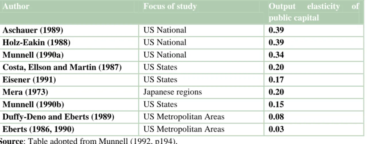
Munnell (1992) provides an excellent assessment of the early literature on the public infrastructure debate. She shows that the main problem with Aschauer (1989)’s work is that his results do not rule out the possibility that the direction of causality runs from growth to infrastructure (i.e. economic growth might lead to an increase in the need for investment and/or an increase in the availability of funding), or that the correlations that he found are spurious. Nevertheless, in response to the critics who claim that the wide range of estimates of public capital’s impact on output ‘make the empirical linkages fragile’, Munnell (1992) provides evidence to suggest these claims are misleading. As illustrated in Table 1 below, in almost all cases the impact of public capital on private output has been found to be positive and statistically significant.
Table 1: The impact of an increase in the stock of public capital on output
Author Focus of study Output elasticity of
public capital
Aschauer (1989) US National 0.39
Holz-Eakin (1988) US National 0.39
Munnell (1990a) US National 0.34
Costa, Ellson and Martin (1987) US States 0.20
Eisener (1991) US States 0.17
Mera (1973) Japanese regions 0.20
Munnell (1990b) US States 0.15
Duffy-Deno and Eberts (1989) US Metropolitan Areas 0.08 Eberts (1986, 1990) US Metropolitan Areas 0.03 Source: Table adopted from Munnell (1992, p194),
Munnell (1992) concludes that the evidence suggests that, in addition to providing an immediate demand-side economic stimulus, public infrastructure investment has a significant, positive
5
effect on output and growth. However, she stresses that in a policy making context ‘Aggregate results cannot be used to guide actual investment spending. Only cost-benefit studies can determine which projects should be implemented’ (Munnell (1992: p196)).
Gramlich (1994)’s influential paper also unpacks many of the arguments and assertions made by Aschauer (1989), along with the mass of academic literature which followed. Gramlich (1994) begins his paper by using the narrow public sector ownership definition as the stock of infrastructure capital – but highlights that a wider meaning could involve private infrastructure capital, human capital investment and research and development spending. This emphasises the importance of definition – what type of investment is being classified as infrastructure and what type is then being linked to economic growth. Gramlich (1994) notes that projects such as a new highway might provide a very high return, whereas maintenance of rural roads might provide low or even negative economic rates of return; in such areas, investment objectives may be primarily social rather than economic. He applies this by showing that only two-thirds of the capital stock analysed by Aschauer (1989) even purports to raising national output – and to varying degrees – making his claims about the major positive influence of infrastructure on economic growth less plausible.
As research in the field progressed, disputes over the direction of causality between changes in productivity and investment in infrastructure became dominant. Evans and Karras (1994) analyzed infrastructure and productivity data for seven Organisation for Economic Co-operation and Development (OECD) countries between 1963 and 1988. The study found strong correlations between the two variables, but concluded that the direction of causality was the opposite of that reported by Aschauer (1989) and Munnell (1992). That is, increased stocks of public capital were the result of increased productivity and economic growth, not the cause. In analysing the correlation between average GDP and government net capital stock, they concluded that “there is no evidence that government capital is highly productive” (Evans and Karras (1994: p278). Zegeye (2000) supports the Evans and Karras (1994) study, concluding that infrastructure is a normal good, where wealthy counties will tend to have more and poor counties less. Zegeye (2000)’s report found the output elasticity between public infrastructure and private investment was just 0.02.
Several other authors have attempted to resolve the question of causality, refining their methodologies to ensure they capture the results of infrastructure investments, and not the results of economic growth. A 2000 OECD study by Demetriades and Mamuneas, and a 2003 study by Esfahani and Ramirez handled the causality issue by introducing a “time-lag” between variables for public infrastructure and productivity. In these studies, investments were compared with the productivity data several years afterwards, allowing time for the benefits of infrastructure investments to manifest themselves in the productivity data, and reducing the chance of misrepresentation of economic growth impacts as productivity impacts. Both studies using this
6
technique found that public infrastructure does have a measurable impact on increasing productivity and economic growth, although not of the magnitude reported by Aschauer (1989). Lau and Sin (1997) published an important econometric paper on public infrastructure and economic growth. This was subsequently referred to as being ‘the most sophisticated subsequent econometric studies’ by SACTRA (1999) and commended for taking the research some way to circumventing the ‘causality’ and ‘definition’ difficulties highlighted by Munnell (1992) and Gramlich (1994)amongst others. The authors estimate the elasticity of output with respect to public capital to be 0.11. Although this would imply a much lower marginal product of public investment than that indicated by Aschauer (1989)’s original paper, it still suggests that infrastructure investment has a significant impact on output.
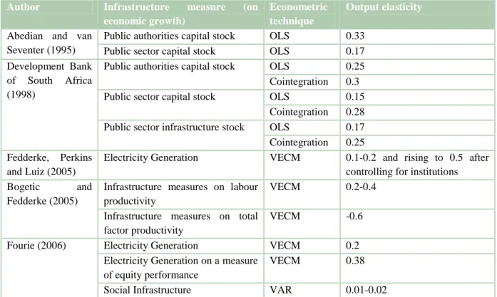
The South African literature on the impact of infrastructure investment on economic growth is still small and relatively recent. It has followed along a similar path to the trends observed for the international literature. A good account of the literature is available in Fourie (2006). Table 2 summarises all the studies that we are aware of on the topic.
Table 2: The impact of an increase in the stock of public capital on output in South Africa Author Infrastructure measure (on
economic growth)
Econometric technique
Output elasticity Abedian and van
Seventer (1995)
Public authorities capital stock OLS 0.33 Public sector capital stock OLS 0.17 Development Bank
of South Africa (1998)
Public authorities capital stock OLS 0.25 Cointegration 0.3 Public sector capital stock OLS 0.15
Cointegration 0.28 Public sector infrastructure stock OLS 0.17 Cointegration 0.25 Fedderke, Perkins
and Luiz (2005)
Electricity Generation VECM 0.1-0.2 and rising to 0.5 after controlling for institutions Bogetic and
Fedderke (2005)
Infrastructure measures on labour productivity
VECM 0.2-0.4 Infrastructure measures on total
factor productivity
VECM -0.6
Fourie (2006) Electricity Generation VECM 0.2 Electricity Generation on a measure
of equity performance
VECM 0.38
Social Infrastructure VAR 0.01-0.02 Source: Table adopted from Fourie (2006) and extended by authors.
The early studies have relied on classical econometric tools while the latter studies have used more recent techniques of Vector Error Correction Models (VECMs) and Vector Autoregressions (VARs). In spite of differences in methodology, the studies report a positive
7
output elasticity. Bogetic and Fedderke (2005) find positive effects of infrastructure on labour productivity but negative effects on total factor productivity. Their explanation for this counterintuitive result is that infrastructure only has direct effects and no indirect effects! This is grossly at odds with predictions from received theory where indirect effects are most important. In follow up work, Fedderke and Bogetic (2006) concluded that infrastructure investment had a positive impact on productivity: total factor productivity increased by 0.04% when investment in economic infrastructure increased by 1%. However, Fedderke and Garlick (2008) suggested that the AsgiSA infrastructure plan might have had unfavourable effects in South Africa. Fourie (2006) finds bi-directional causality between infrastructure and growth and also finds large positive returns to infrastructure on equity. Thus, the South African econometric studies show favourable effects of infrastructure spending on growth, irrespective of the methodology used. Some even go further to argue that infrastructure on equity has higher returns than economic infrastructure7.
Compared to the econometrics literature, the literature on CGE applications of public capital expenditures and links to economic growth is more recent and still growing. Similar to the econometrics literature just reviewed, the findings of this literature are mixed. Whilst most find that the output elasticity of public expenditure is positive, the magnitudes of the effects vary considerably. In a summary of some of the main studies on infrastructure, Kirsten and Davies (2008) show that, in general, studies that looked at various infrastructure sectors (roads, sanitation, electrification and dams) display varied results – some are beneficial for poverty reduction, others actually cause poverty. Using a static CGE model, Perrault et al. (2010) explore the impact of scaling up infrastructure in six African countries with different economic structures. They find that the different economic structures lead to differences in impact of investment funded by the same sources with the same model. The analysis shows the importance of the underlying economic structure in determining the impact of infrastructure expenditure in a country. This suggests that the structure of the economy where these policies will be applied needs to be taken into account.
Another strand of related literature concerns itself with the effects of scaling up aid to developing countries. Received wisdom based on standard analysis came to the conclusion that scaling up aid flows would generate sustained growth and improved standard of living (Adam (2005)). This view has been challenged by authors who point out that both intended and unintended consequences discussed largely under the rubric of what has come to be referred to as
7
Ayogu (2005) also surveys the theoretical literature on infrastructure and growth and then reviews the empirical evidence globally and within the African region. Overall he concludes that the question is not whether infrastructure matters but precisely how much it matters in different contexts? Ultimately, this is an empirical question that the literature has not yet resolved satisfactorily. In contrast, according to him, the crucial issue—understanding policymaking processes in infrastructure—remains little understood and largely under-researched.
8
‘absorptive capacity constraints’(see for example Burnside and Dollar (2004); Clemens and Redelet (2003); Heller (2005);Allen (2005)) make the impact of aid on economic growth indeterminate. A major concern in this respect is the so-called Dutch disease effect associated with scaling up foreign aid8. Recent evidence (including Adam and Bevan (2003); Allen (2005); Heller (2005); Bourguignon and Sundberg (2006)) has shown that the conventional Dutch disease effects may be overturned if there are productivity spillovers in both tradable and non-tradable sectors. Using Uganda as an example, Adam and Bevan (2006) construct an aggregated CGE model and demonstrate that Dutch disease type effects can be avoided if the non-tradable sectors benefit from infrastructure investment externalities. Savard (2010) extends this kind of reasoning in three ways, namely, dropping the tradable-nontradables dichotomy, allowing for a wider variety of funding options for infrastructure spending and introducing a top-down bottom up microsimulation module to allow for poverty analysis. Applying the methodology to explore the impact of scaling up infrastructure in the Philippines, Savard (2010) finds that the macro results obtained from the analysis are similar to Adam and Bevan (2006) and Estache (2008), although the Dutch disease effects disappear when they assume the presence of production externalities. There are also no major differences at the macro level when taking into account funding options to scale-up infrastructure. However, poverty analysis shows stark differences and in particular the VAT funding option yields the most favourable outcomes in terms of poverty reduction when compared to the foreign aid option and the income tax option. To improve the analysis on this front, Savard (2010) suggests that a sequentially dynamic framework would be a more appropriate tool.
A number of recent studies have sought to make contributions along this line. For instance, Jung and Thorbecke (2003) use a recursive dynamic CGE framework and showed that infrastructure spending benefited poor people in Tanzania but worsened the plight of the poor in Zambia. A fair amount of authors investigating the impacts or challenges of scaling up aid to achieve the Millennium Development Goals (MDG) (see for example Bourguignon and Sundberg (2006), Hailu (2007) and Serieuxet al.(2008)) have also used this recursive dynamic approach. The model that is typically used in these exercises is referred to as the MAMS model (for details on the MAMS model, see Lofgren and Diaz-Bonilla (2005)). This model extends static standard CGE models of the type discussed above in two key respects. First is the incorporation of recursive dynamics and second is the addition of an MDG module that endogenizes MDG outcomes. The paper by Bourguinon and Sundberg (2006) based on the MAMS model calibrated to Ethiopian data concludes among other things, that the impact of large aid inflows on the Dutch disease can be serious but strategic investments to boost productivity and address trade constraints are important in addressing the adverse effects. World Bank (2005) report a similar finding for Ethiopia based on a model that focused on aid-financed investments in human capital.
8
The term Dutch disease refers to a phenomenon where an economic boom (normally a discovery of natural resource or large inflow of foreign currency) leads to a real exchange rate appreciation that results in increased demand for non-tradables and eventually to a decline in the economic growth rate. It was coined to describe the de-industrialisation experienced in the Netherlands in the 1960s following the discovery of natural gas in the North Sea.
9
Mabugu et al (2013) use an intertemporal CGE model to investigate the consequences of an expansive fiscal policy designed to accelerate economic growth in South Africa. The model is oriented towards constraints government faces in financing its expenditures and explains why it takes into account the different sources of income of the South African government, its expenditures and its deficit as well as intertemporal dynamics. The labour market faces a lot of rigidities in South Africa that the intertemporal model does not capture.
Our paper is fundamentally similar in spirit and conception to these CGE-based simulation models just described but applied to reflect the structural features of the current South African economy. Presumably, the extent to which productivity spillovers from infrastructure investments can potentially affect the economy will depend on the particular circumstances of the country. In this respect we draw from the extensive infrastructure productivity econometrics literature discussed to postulate positive productive externalities associated with new infrastructure for South Africa. Unlike Mabugu et al (2013), labour market peculiarities of the South African economy have been included in our modelling and dynamics are modelled as recursive rather than intertemporal. This paper is intended to contribute to the discussion by providing evidence from South Africa using the economy-wide dynamic CGE model calibrated to contemporary conditions in the country.
3 Data and Methodology9
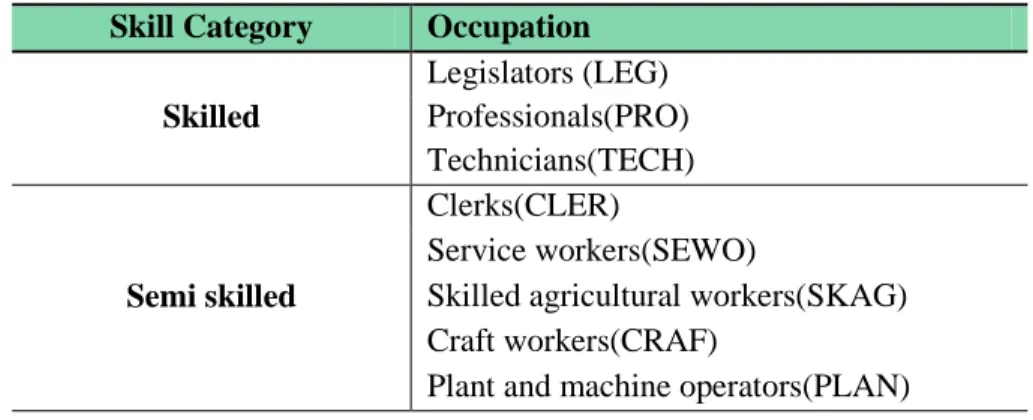
The original Social Accounting Matrix (SAM) used is from Quantec for 2005. The different occupations in the SAM are identified as skilled, semi-skilled and unskilled. For the purpose of this paper, the labour factor is disaggregated further into occupations. Integrated economic accounts from Statistics South Africa (StatsSA) for 2005, where the labour force is split according to occupation and population groups, are used after ensuring concordance with the SAM economic activities codes (Table 3)
Table 3: Correspondence between occupations and skills level
Skill Category Occupation
Skilled Legislators (LEG) Professionals(PRO) Technicians(TECH) Semi skilled Clerks(CLER) Service workers(SEWO)
Skilled agricultural workers(SKAG) Craft workers(CRAF)
Plant and machine operators(PLAN)
9
10 Unskilled
Elementary occupations(ELEM) Domestic workers(DOM) Occupation unspecified(ONS)
11
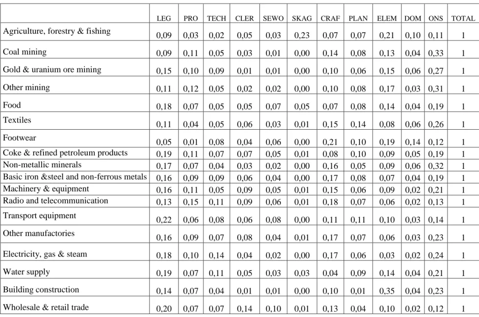
Table 4: Repartition of the labour force according to occupations and activities:
LEG PRO TECH CLER SEWO SKAG CRAF PLAN ELEM DOM ONS TOTAL
Agriculture, forestry & fishing
0,09 0,03 0,02 0,05 0,03 0,23 0,07 0,07 0,21 0,10 0,11 1
Coal mining 0,09 0,11 0,05 0,03 0,01 0,00 0,14 0,08 0,13 0,04 0,33 1
Gold & uranium ore mining 0,15 0,10 0,09 0,01 0,01 0,00 0,10 0,06 0,15 0,06 0,27 1
Other mining 0,11 0,12 0,05 0,02 0,02 0,00 0,10 0,08 0,17 0,03 0,31 1 Food 0,18 0,07 0,05 0,05 0,07 0,05 0,07 0,08 0,14 0,04 0,19 1 Textiles 0,11 0,04 0,05 0,06 0,03 0,01 0,15 0,14 0,08 0,06 0,26 1 Footwear 0,05 0,01 0,08 0,04 0,06 0,00 0,21 0,10 0,19 0,14 0,12 1
Coke & refined petroleum products 0,19 0,11 0,07 0,07 0,05 0,01 0,08 0,10 0,09 0,05 0,19 1
Non-metallic minerals 0,17 0,07 0,04 0,03 0,02 0,00 0,16 0,05 0,09 0,06 0,32 1
Basic iron &steel and non-ferrous metals 0,16 0,09 0,09 0,06 0,04 0,00 0,17 0,08 0,07 0,04 0,19 1
Machinery & equipment 0,16 0,11 0,05 0,09 0,05 0,01 0,15 0,06 0,09 0,02 0,21 1
Radio and telecommunication 0,13 0,15 0,11 0,09 0,06 0,01 0,18 0,07 0,06 0,02 0,13 1
Transport equipment
0,22 0,06 0,08 0,06 0,08 0,00 0,11 0,11 0,10 0,03 0,14 1
Other manufactories
0,16 0,09 0,07 0,08 0,04 0,01 0,17 0,07 0,06 0,03 0,23 1
Electricity, gas & steam 0,18 0,10 0,14 0,04 0,02 0,00 0,17 0,06 0,03 0,02 0,24 1
Water supply 0,19 0,07 0,11 0,05 0,03 0,03 0,04 0,09 0,14 0,04 0,21 1
Building construction 0,14 0,07 0,04 0,01 0,01 0,00 0,10 0,01 0,35 0,04 0,23 1
12
Catering & accommodation services 0,23 0,04 0,05 0,10 0,25 0,01 0,04 0,03 0,09 0,03 0,12 1
Transports services 0,08 0,03 0,03 0,11 0,07 0,00 0,07 0,23 0,09 0,04 0,25 1
Communication 0,23 0,12 0,09 0,19 0,07 0,01 0,04 0,06 0,04 0,01 0,14 1
Finance and insurance 0,27 0,20 0,11 0,25 0,05 0,00 0,02 0,01 0,01 0,01 0,09 1
Business services
0,18 0,26 0,08 0,09 0,15 0,01 0,05 0,03 0,02 0,02 0,11 1
Other services 0,04 0,09 0,02 0,06 0,06 0,01 0,05 0,03 0,02 0,08 0,53 1
Public services 0,17 0,12 0,06 0,15 0,33 0,01 0,04 0,03 0,02 0,02 0,05 1
13
From Table 4, we can point out that the construction sector is likely to be disproportionately affected by an infrastructure investment program policy because the sector is quite intensive in low skilled workers, especially the ones identified as elementary or unspecified occupations. Moreover, legislators (LEG) represent 15% of the labour force in this particular sector.
For modelling, Gibson (2003) is used for the trade parameters and low-bound export supply, while demand elasticities are obtained from Behar and Edwards (2004). Estimates for parameters in industry production and household demand are not available for South Africa. Therefore, the study borrows these values from the literature surveyed by Annabi et al. (2006). Finally, unemployment rates are drawn from the labour force survey report by StatsSA (2009).
To evaluate the impacts of government’s policies in the long run, the dynamic Poverty and Economic Policy (PEP 1-t) standard model by Decaluwé et al. (2010) is used. However, several assumptions of this standard model are changed in order to take into account the South African economy. The model has two production factors: capital and labour. Labour is disaggregated into three broad types: unskilled, semi-skilled and skilled workers. Each type of broad labour is then disaggregated into occupations. Each activity uses both production factors.
In line with the SAM, the model has 25 activities and 54 commodities. The production function technology is assumed to be of constant returns to scale and is presented in a four-level production process. At the first level, output is a Leontief input-output of value added and intermediate consumption. At the second level, a CES function is used to represent the substitution between a composite labour and capital. At the third level, composite labour demand is also a CES function between skilled, semi-skilled and unskilled labour. Then, the skilled demand is a CES with a low elasticity between legislators, professionals and technicians, capturing the fact that (for instance) it is quite difficult for the firms to substitute a lawyer for a doctor. The semi-skilled demand is a CES with an intermediate value of elasticity between its five components, while the unskilled demand is a CES with a high substitution value, assuming that the producer can relatively easily substitute low skilled workers among them. Figure 1 gives the value-added structure.
14
Figure 1: The value-added structure
South Africa has high unemployment problems, notably for semi-skilled and unskilled labour. Moreover, unions are very strong in the country. The trade union movement is the most disciplined and the largest in Africa and has influenced labour and other related industrial policies. Unions negotiate salaries and wages, conditions of service, workforce restructuring and retrenchments on behalf of their members. As a result, wages and salaries are rigid, which the model takes into account by assuming a binding minimum wage for each type of worker. Thus, if the production decreases, producers will not be able to decrease their employees’ salary below the minimum wage. This rigidity will also have an impact on unemployment, as if producers cannot decrease the wage bill, they will have to retrench some workers.
Following the literature review in the previous section, we introduce a productivity factor to investment in infrastructure. As mentioned, the value added for each sector is a CES composite of labour and capital. We add a productivity factor related to the stock of infrastructure in the country to the function.
𝑉𝐴𝑗,𝑡= �𝐾𝐷𝑡 𝐼𝑁𝐹 𝐾𝐷𝑡−1𝐼𝑁𝐹� 𝜎𝑗𝐼𝑁𝐹 𝐵𝑗𝑉𝐴�𝛽𝑗𝑉𝐴𝐿𝐷𝐶𝑗,𝑡−𝜌𝑗 𝑉𝐴 + �1 − 𝛽𝑗𝑉𝐴�𝐾𝐷𝐶𝑗,𝑡 −𝜌𝑗𝑉𝐴 � −1 𝜌𝑗𝑉𝐴 Value Added Composite Labour Skilled labour
Legislators Professionals Technicals
Semi-skilled workers Clerks Service workers Skilled agricultural Craft workers
Plant and machine operators
Unskilled labour Elementary
occupations Domestic workers Unspecified Capital
15 Where:
:
,t
j
VA Value added of sector j
: INF t KD Infrastructure stock : ,t j
LDC Sector j aggregate labour demand :
,t
j
KDC Demand for composite capital by sector j
: VA
j
B Scale parameter (CES – value added)
: VA j
β Distributive parameter (CES – value added)
: VA j
ρ Elasticity parameter (CES – value added)
: INF j
σ Elasticity – productivity and infrastructure
Modelled in this way, investment in infrastructure will increase the stock of infrastructure capital (𝐾𝐷𝑡𝐼𝑁𝐹), in the following year. If no investment is made, then the stock of infrastructure capital remains the same and there is no extra increase in value added of a given sector. The value of elasticity 𝜎𝑗𝐼𝑁𝐹 is obtained from the existing literature.
As closure rules, we choose the nominal exchange rate as the numeraire in the model.10 Following the assumption that South Africa is a small country, world prices are fixed. However, also assumed is the fact that South African exporters face less than infinite foreign demand for exports: to increase their market share on the world market, they need to reduce their free-on-board (FOB)export prices, increasing their competiveness with respect to other suppliers on the international market. Factor supplies are fixed in the first period and then grow, at the population rate for labour force and using an accumulation equation for capital.11 Transfers between institutions and government’s purchases of commodities are fixed at the base year and then grow at the population rate. The assumption is that the rest of the world’s savings is a fixed proportion of GDP, which means that South Africa is not allowed to borrow further from the rest of the world.12
4 Policy Simulations and Results
.
This paper analyses the impact of an increase in public investment, following the South African investment plan presented in the table below for the period 2012 up to 2016, and thereafter at the population rate. The simulated investment programme is split into three components (a)
10Note that in the CGE results, a real devaluation of the rand takes the form of a generalised reduction in domestic prices.
11 To specify the accumulation of capital, the Jung and Thorbecke (2003) function is followed.
12 This assumption can seem strange given that the country has in the past increased their savings from abroad. However, South Africa does not want to increase substantially its current level of borrowing.
16
investment in government sectors (e.g. education, justice) that increase the stock of capital of public sectors, (b) investment in infrastructure (e.g. roads, harbours, airports) that does not increase the stock of capital of any sectors in particular and can be considered a public good and (c) investment in productive sectors (e.g. investment in the energy sector) that increase the capital stock of a given sector. Based on the literature reviewed, the simulations thus take into account the effect of infrastructure productivity on the other sectors. Assuming productivity effect of infrastructure investment on other sectors means, for instance, that the construction of a bridge (investment in infrastructure) will have an impact on other sectors if the use of this bridge reduces travel time) or government investment in building a road (infrastructure spending), or in constructing/renovating a harbour, has impacts on other sectors: their transport margins will decrease and they will be able to trade more, using the same quantities of labour and capital. Government investment can also increase private capital stock, for instance when government invests in a nuclear plant, it increases the stock of capital of the electricity/energy sector.
Table 5: South African investment plan:
Nov.-2010 Dec-2011 2012/13 2013/14 2014/15
Economic services 161,9 197,3 217,8 228,2 230,1
Energy 52,5 71,7 90,4 98,8 102,7
Water and sanitation 14,4 17,8 20,6 19,9 19,8
Transport and logistics 69,1 79,5 76,3 76,9 72,3
Other economic services 25,8 28,4 30,4 32,5 35,2
Social services 17,2 26,6 26,8 32,5 35,2
Health 6,7 10 9,6 13,9 15,2
Education 6 9,1 9,8 11,2 11,2
Community facilities 3,5 5,2 4,7 4,8 6,2
Other social services 1 2,4 2,6 2,6 2,7
Justice and protection
3,8 4,1 4,4 5,1 5,8
services
Central government and 2,1 4,2 8 3,5 2,5
Financial services 0,3 0,7 0,7 0,7 0,8
Total 185,3 232,9 257,6 269,9 274,4
Source: Medium Term Budget Policy Statement (2011), page 26 table 3.2
Four different ways of financing these policies are proposed. First, government totally finances the increase (i.e. government’s savings are endogenous and, given the policy set up, might decrease). Then, in the next three finance options, government’s deficit is kept constant, and the increased spending is financed through increasing direct taxes on households, increasing firms’ direct taxes, and increasing indirect taxes.
17 1- Deficit financed investment policy
The results of an increase in government’s public investment on unemployment are shown in Table 6. The policy has a very positive impact on unemployment for all the different types of workers both in the short run (2012) and long run (2020). Government’s activities are more intensive in skilled and semi-skilled workers, and so the impact is greater for these two types of workers. For skilled workers, unemployment disappears in 2015 and for all categories, positive impacts remain after the simulations years.
Table 6 : Impact on unemployment (% to Business as Usual (BAU))
LEG PRO TECH SEWO SKAG CRAF PLAN CLER
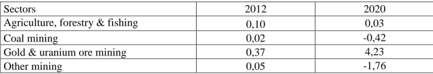
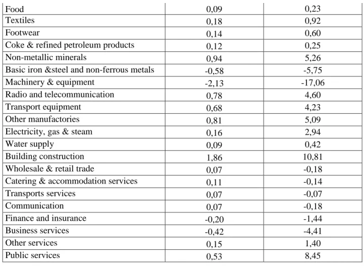
ELE M DOM ONS 2012 -13,93 -0,06 -5,06 -0,92 -1,72 -1,35 -1,27 -0,51 -1,88 -0,85 -0,74 2020 -14,31 -25,64 -11,89 -15,46 -12,83 -15,08 -8,74 -7,07 Table 7 presents the impacts on production for each sector of the economy. In the short run, most of the sectors increase their production, but in the long run quite a number of them experience a decrease. The reason why impacts on production are quite positive for most of the sectors is because these activities do not suffer total crowding out effect as some public investment is directly improving their production (as the electricity sector) and all the sectors benefit from a decrease in margins costs, due to the improvement of infrastructure in the economy. The increase in government spending also has an impact on the other sectors through an increase of intermediate demand. To produce more, government sectors need extra public servants, buildings, and all types of commodities produced by the other sectors. With the decrease of unemployment, workers also receive an increase in wages. Indeed, as government’s activities need more workers to produce, they will attract skilled and semi-skilled workers mainly by offering a better wage than the other activities. Thus, to keep their workers, the other activities will also have to increase the wages they pay to their workers, which results in increased production costs. Sectors with a similar labour demand structure will find it more costly to produce and this explains why their production levels decline. The decline is also due to a drop in total investment induced by government crowd out.
Table 7 : Impact on Production (% to BAU)
Sectors 2012 2020
Agriculture, forestry & fishing 0,10 0,03
Coal mining 0,02 -0,42
Gold & uranium ore mining 0,37 4,23
18
Food 0,09 0,23
Textiles 0,18 0,92
Footwear 0,14 0,60
Coke & refined petroleum products 0,12 0,25
Non-metallic minerals 0,94 5,26
Basic iron &steel and non-ferrous metals -0,58 -5,75
Machinery & equipment -2,13 -17,06
Radio and telecommunication 0,78 4,60
Transport equipment 0,68 4,23
Other manufactories 0,81 5,09
Electricity, gas & steam 0,16 2,94
Water supply 0,09 0,42
Building construction 1,86 10,81
Wholesale & retail trade 0,07 -0,18
Catering & accommodation services 0,11 -0,14
Transports services 0,07 -0,07
Communication 0,07 -0,18
Finance and insurance -0,20 -1,44
Business services -0,42 -4,41
Other services 0,15 1,40
Public services 0,53 8,45
The impacts on agents are quite interesting as they differ. Households benefit from this policy because of the decrease in unemployment and the increase in wages raise household income (Table 8). Note that although their transfer income from firms (dividends) decreases, overall household income increases in the long run by almost 1%. Household savings and consumption also increase, as they are fixed proportions of disposable income.
Table 8 : Impact on households’ income (in % to BAU)
Labor income Transfer income Total income
2012 0,20 -0,17 0,06
2020 3,49 -3,26 0,91
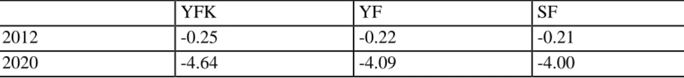
Firms are suffering but less than in the case had investment in infrastructure been assumed to have no productivity effect. The negative impact on firms is less in the short compared to the long run. Capital income decreases, and so do firms’ income and savings, because of the drop in total investment (Table 9).
19
Table 9 : Impact on firms’ income and savings (in % to BAU)
YFK YF SF
2012 -0.25 -0.22 -0.21
2020 -4.64 -4.09 -4.00
Table 10 presents all the sources of government’s income and how they react to the increase in government spending. The first component represents transfer income and comes mainly from firms (dividends). The second one represents all the taxes on production (on labour, capital, production). The third one is the sum of all taxes on products (import taxes, VAT, export taxes, excise taxes, fuel levy). The final one is total direct taxes paid by households and firms. Government income is slightly decreasing in the long run, due to the decrease in transfers government receives from firms and the receipts from firms’ direct taxes.
Table 10 : Impact on government (in % to BAU)
Transfers income Taxes on production Taxes on products Direct taxes on households Direct taxes on firms Total government income 2012 -0,21 -0,24 0,12 0,06 -0,25 -0,01 2020 -4,00 -1,26 0,86 0,91 -4,64 -0,63
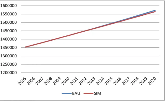
Not surprisingly, we observe a drop in government’s savings as there is no tax policy adjustment to finance the investment program. The drop in government savings, followed by the drop in firms’ savings, leads to a decrease in total investment. While a crowding-out effect of investment is evident, the impact on private investment is less harmful because a part of government investment is productive. The impact on GDP is hardly perceptible as shown in Figure 2. With this type of policy, the idea is to see what happens in the long run. It is known that in the short run, government deficit increases a lot, but in the long run, the pressing policy issue is ‘can this spending create a greater economic activity in order to generate new revenue’? For instance, a policy that creates jobs will have an impact on the fiscal side, as new workers will get income and pay new taxes (direct and indirect). The next set of simulations address this issue.
20
Figure 2 : Impact on GDP
2- Tax financed investment policy
The first simulation has very positive results on unemployment and benefits to households. However, in the long term, the drop in total investment tends to reduce economic growth. Moreover, it is not sustainable for South Africa to let its deficit grow unabated. Therefore, the same simulation is presented, but the closure of the model is changed: government’s savings are kept fixed, and an endogenous tax finances the policy. In Simulation FinA, the direct tax rate of households adjusts. In Simulation FinB, the direct tax rate on firms adjusts, and in Simulation FinC, the indirect tax rate adjusts. The results of these three simulations are presented together. In terms of unemployment, as shown in the following tables, the results differ according to the scenario. FinB scenario seems to be the less harmful across all categories of workers. Note that for skilled workers, as the values of unemployment were low at the base year, the percentage change look dramatic. Note though that results are still very negative under Simulation FinC. Indeed, under this scenario, both agents and activities are hit by the increase in commodity tax rate.
Table 11 : Impact on unemployment for skilled workers (% to BAU)
LEG PRO TECH
2012 2020 2012 2020 2012 2020 FinA 42,75 50,39 67,29 171,88 37,11 73,07 FinB 17,09 36,75 -32,04 18,05 -34,51 FinC 156,38 877,84 185,02 1076,57 119,78 606,59 1200000 1250000 1300000 1350000 1400000 1450000 1500000 1550000 1600000 BAU SIM
21
Table 12 : Impact on unemployment for semi-skilled workers (% to BAU)
CLER SEWO SKAG CRAF PLAN
2012 2020 2012 2020 2012 2020 2012 2020 2012 2020
FinA 4,46 13,99 1,49 -4,79 7,73 38,36 0,37 -8,44 2,82 6,33
FinB 2,21 -0,81 0,40 -11,15 3,46 8,20 -0,40 -13,02 0,98 -6,14
FinC 10,58 60,01 5,74 29,80 14,83 88,72 8,00 47,01 10,20 60,83
Table 13 : Impact on unemployment for low skilled workers (% to BAU)
ELEM DOM ONS
2012 2020 2012 2020 2012 2020
FinA -2,77 -24,10 1,40 3,00 1,71 5,26
FinB -2,36 -21,81 0,39 -3,53 0,60 -1,61
FinC 1,58 7,61 4,76 28,01 5,10 30,42
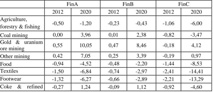
The impact on the sectors depends on how heavily sectors rely on investment. Activities that face an increase in their input prices (in terms of intermediate consumption) will retrench workers, and reduce their production. The impact is not uniform across sectors. Indeed, some sectors are directly favoured by the investment policy, especially the construction sector. Moreover, some sectors do not directly benefit from the policy, but as they produce investment goods, their production will increase. Once again, results under FinC are very harmful for the economy.
Table 14 : Impact on production (% to BAU)
FinA FinB FinC
2012 2020 2012 2020 2012 2020
Agriculture,
forestry & fishing -0,50 -1,20 -0,23 -0,43 -1,06 -6,00
Coal mining 0,00 3,96 0,01 2,38 -0,82 -3,47
Gold & uranium
ore mining 0,55 10,05 0,47 8,46 -0,18 4,12
Other mining 0,42 7,05 0,25 3,39 -0,19 0,97
Food -0,94 -4,52 -0,48 -2,20 -1,44 -8,53
Textiles -1,50 -6,84 -0,74 -2,97 -2,41 -14,41
Footwear -1,32 -6,27 -0,66 -2,89 -2,21 -13,29
22 petroleum
products Non-metallic
minerals 3,03 25,42 2,08 16,73 1,97 16,45
Basic iron &steel and non-ferrous metals 0,79 9,13 0,16 2,93 -0,38 -0,51 Machinery & equipment 0,68 7,52 -0,60 -2,97 -0,65 -3,18 Radio and telecommunication 0,78 9,18 0,78 7,63 -0,49 -1,23 Transport equipment 0,80 9,06 0,74 7,33 -0,64 -2,51 Other manufactories 0,58 8,00 0,68 7,06 -0,17 1,56
Electricity, gas &
steam -1,08 -2,92 -0,51 0,12 -1,64 -8,62
Water supply -0,99 -3,43 -0,50 -1,35 -1,52 -8,47
Building
construction 5,87 43,49 4,05 29,36 4,40 32,09
Wholesale & retail
trade -0,23 1,34 -0,09 0,99 -0,91 -4,55 Catering & accommodation services -1,34 -6,01 -0,68 -2,94 -2,11 -12,53 Transports services -0,21 1,27 -0,08 0,93 -0,77 -3,77 Communication -0,92 -3,24 -0,47 -1,48 -1,48 -8,63 Finance and insurance -0,98 -3,13 -0,63 -1,74 -1,76 -9,49 Business services -0,52 -0,77 -0,48 -2,15 -1,06 -6,25 Other services -1,57 -7,57 -0,79 -3,31 -1,97 -11,32 Public services 0,57 10,32 0,55 9,89 0,28 6,87
The impact on households is negative because the drop in transfers they receive from firms, and the decrease in labour income they receive (Table 15). Note that in the long run household income falls the least under FinA, that is, when direct tax rate adjusts.
23
Table 15 : Impact on households’ income (% to BAU)
Labour income Transfer income Total income
2012 2020 2012 2020 2012 2020
FinA -0,42 -0,34 -0,42 -3,31 -0,42 -1,47
FinB -0,14 1,45 -3,21 -23,21 -1,31 -7,96
FinC -1,59 -9,11 -1,01 -8,09 -1,37 -8,72
The impact on firms is also negative, notably under Simulation FinB, as they face an increase in the direct taxes they pay. Here, firms’ savings drop by almost 30% in the long run, which will have a massive impact on private investment. In the three scenarios, government income increases due to the fiscal mechanism set up. Private investment decreases and is worse when firms have to finance the policy. This is because firms contribute significantly to private investment. Overall, total investment increases for each scenario. As public investment increases due to the policy, total investment also increases. The increase is less significant under FinB (Figure 3).
Figure 3 : Impact on total investment
Finally, from Figure 4 it can be observed that the policy is less harmful to GDP when financed by firms. Indeed, when households finance the policy, the impact on consumption and thus on GDP is too big. Needless to say, in Simulation FinC, the results are very bad. Financing the policy through an increase in indirect tax penalises the entire economy.
250000 270000 290000 310000 330000 350000 370000 390000 410000 430000 450000
24
Figure 4 : Impact on GDP (at basic prices)
5 Concluding remarks and policy discussion
This paper has analysed the investment policy the South African government plans to set up under four different fiscal scenarios. The way this investment plan has been treated in our modelling allows the government to intervene in public and private sectors of the economy. The benefits of infrastructure investment are taken into account through a productivity mechanism that will enhance other sectors. Particular attention has been paid to the labour market in the modelling.
Besides improving the quality of infrastructure, the government wishes to reduce unemployment that is endemic in the country. In terms of employment, the results are quite disappointing: indeed, except under the first scenario, this investment plan is not able to generate enough activity in the economy to reduce unemployment. If we consider a long term fiscal sustainability, VAT financing of the investment plan is pretty harsh on the economy, as it affects all the agents in the economy. Moreover, this fiscal policy would not be ‘pro-poor’ because all households (including the poor) are hit by an increase in VAT. The alternative financing scenario would offer some political options to the government, as it will target only households that pay direct taxes or firms. An intermediate solution could this incorporate a combined burden sharing between households and firms.
. 1200000 1250000 1300000 1350000 1400000 1450000 1500000 1550000 1600000
25
References
Abedian, I. and Van Seventer, D., (1995). “Productivity and multiplier analysis of infrastructure investment in South Africa: an econometric investigation and preliminary policy implications”. Mimeo. Pretoria: Ministry of Finance.
Adam, C. (2005). Exogenous Inflows and Real Exchange Rates; Theoretical Quirk or Empirical Reality? An IMF Paper, Available at www. Imf.org/FAMM
Adam, C., and Bevan D., (2003) “Aid, Public Expenditure and Dutch Disease” Centre for the Study of African Economies, Working Paper Series, Paper 184
Adam, C. and Bevan, D., (2006), “Aid and the Supply Side: Public Investment, Export Performance and Dutch Disease in Low Income Countries,” World Bank Economic Review, Vol. 20(2), pp. 261-290.
Aghion and Howit (2000), Endogenous Growth Theory, Cambridge Massachusetts, The MIT Press
Allen M., (2005) “The Macroeconomics of Managing Increased Aid Inflows: Experiences of Low-income Countries and Policy Implications”, A Paper Prepared by the Policy Development and Review Department of the International Monetary Fund (IMF).
Annabi, N, Decaluwé, B, and Cockburn, J. (2006), Functional forms and parameterization of CGE models, PEP, MPIA Working Paper 2006-04.
Arrow, K.J. and M. Kurz (1970), Public Investment, the Rate of Return and Optimal Fiscal
Policy, Baltimore: John Hopkins Press.
Aschauer, D.A., (1989), “Is Public Expenditure Productive”, Journal of Monetary Economics, 23, 177-200.
Ayogu, M., (2005), “Infrastructure and Economic Development in Africa: A Review”, Invited Paper for the December 2005 AERC Biannual Plenary Session on Services and Economic
Development in Africa, Rosebank Hotel, Johannesburg 3–8 December 2005.
Behar, A and Edwards, L. (2004)."Estimating elasticities of demand and supply for South African manufactured exports using a vector error correction model."Working Paper 204.The Centre for the Study of African Economies.
Bogetic, Z. and Fedderke, J. (2005), “ Infrastructure and Growth in South Africa: Benchmarking, Productivity and Investment Needs”. Presented at the ESSA conference 2005. Available online: http://www.essa.org.za/
Bourguignon, F. and Sundberg, M. (2006).“Constraints to Achieving the MDGs with Scaled-Up
Aid”, DESA Working paper, No. 15.Available at
http://www.un.org/esa/desa/papers/2006/wp15 2006.pdf.
Burnside, C. and Dollar, D., (2004), “Aid, Polices and Growth, Revisiting the Evidence”, Policy Research Working Paper 3251, World Bank, Washington DC.
Clemens, M., and Redelet, S., (2003): “The Millenium Challenge Account: How much is too much, how long is long enough?”, Working Paper No.23, Center for Global Development, Washington DC.
Decaluwé, B., A. Lemelin, V. Robichaud and H. Maisonnave (2010), PEP-1-t. Standard PEP
model: single-country, recursive dynamic version, Politique économique et Pauvreté/Poverty
26
Demetriades, P., and Mamuneas, T., (2000)."Intertemporal Output and Employment Effects of Public Infrastructure Capital: Evidence from 12 OECD Economics”,Economic Journal, Royal Economic Society, vol. 110(465), pages 687-712, July.
Development Bank of South Africa (1998), “Infrastructure: a foundation for development”. Development Report 1998: Pretoria.
Esfahani, H.S., and Ramirez, M.T., (2003). "Institutions, infrastructure, and economic growth", Journal of Development Economics, Elsevier, vol. 70(2), pages 443-477, April.
Estache, A., (2007), "Infrastructure and Development: A Survey of Recent and Upcoming Issues", in Bourguignon, F., and B. Pleskovic, Rethinking Infrastructure for Development – Annual World Bank Conference on Development Economics, Global, pp. 47-82.
Evans, P., and Karras, G., (1994). "Is government capital productive? Evidence from a panel of seven countries", Journal of Macroeconomics, Elsevier, vol. 16(2), pages 271-279.Fedderke, J. and Bogetic, Z. (2006), “Infrastructure and Growth in South Africa: Direct and Indirect Productivity Impacts of 19 Infrastructure Measures”. World Bank Policy Research Working Paper 3989, Washington, DC: The World Bank.
Fedderke, J and Garlick, R. 2008. “Infrastructure development and economic growth in South Africa: a review of the accumulated evidence”, Policy Paper No 12. School of Economics, University of Cape Town and Economic Research Southern Africa.
Fedderke, J., Perkins, P. and Luiz, J. (2005). “Infrastructure Investment in Long-run Economic Growth: South Africa 1875–2001”. Preliminary draft. Available online: http://www.uct.ac.za/economics.
Fourie, J., (2006), “Some policy proposals for future infrastructure investment in South Africa”, Stellenbosch Economic Working Papers: 05/06, Department of Economics, University of Stellenbosch.
Gibson, KL. (2003). “Armington elasticities for South Africa: long- and short-run industry level estimates, trade and industrial policy strategies”, Working Paper 12-2003.
Gramlich, E., (1994), “Infrastructure Investment: A Review Essay”, Journal of Economic Literature, 32.
Hailu, D. (2007). "Scaling-up HIV and AIDS Financing and the Role of Macroeconomic Policies in Kenya", IPC Conference Paper 4. Paper presented at the Global Conference on Gearing Macroeconomic Policies to Reverse the HIV/AIDS Epidemic, 20–21 November, Brasilia: International Poverty Centre (IPC) (mimeo).
Heller, P. S. (2005). Pity the Finance Minister: managing a substantial scaling up of aid flows. Processed, Fiscal Affairs Department, International Monetary Fund, Washington, DC.
Jung, H.S., and Thorbecke, E., (2003). "The impact of public education expenditure on human capital, growth, and poverty in Tanzania and Zambia: A general equilibrium approach",
Journal of Policy Modeling, 25, pp 701–725.
Kirstern, M and Davies, G. 2008. Asgisa – is the bar set high enough? Will the accelerated infrastructure spend assist in meeting the targets? Development Bank of Southern Africa. Tips Conference.29–31 October 2008, Cape Town.
Lau, S.H.P., and Sin, C.Y., (1997), “Public Infrastructure and Economic Growth: Time Series Properties and Evidence”, Economic Record, 73.
Lofgren, H., and Diaz-Bonilla, C., (2005). An Ethiopian Strategy for Achieving the Millennium Development Goals: Simulations with MAMS model, Processed, February, World Bank, Washington DC.
27
Mabugu, R., Robichaud, V., Maisonnave, H., and Chitiga, M., (2013) "Impact of Fiscal Policy in an Intertemporal CGE Model for South Africa", Economic Modelling 31: 775-782
Moreno-Dodson, B. (2009), “On the Marriage between Public Spending and Growth: What Else Do We Know?”, The World Bank PREM Notes in Economic Policy, No. 130.
Munnell, A.H., (1992), “Policy Watch: Infrastructure Investment and Economic Growth”, The Journal of Economic Perspectives, Volume 6 No. 4.
National Treasury (2011), Medium Term Budget Policy Statement, Republic of South Africa,
available online at http://www.treasury.gov.za/documents/mtbps/2011/mtbps/MTBPS%202011%20Full%20Do
cument.pdf
Perrault, J., Savard, L., and Estache, A., (2010). "The impact of infrastructure spending in Sub-Saharan Africa: A CGE modelling approach." Policy Research Working Paper Series 5386. Washington, DC: The World Bank.
SACTRA (1999), Transport and the Economy, United Kingdom, DETR (Department of Environment, Transport and Regions). London. www.dft.gov.uk
Savard, L., (2010), “Scaling Up Infrastructure Spending in the Phillipines: A CGE Top Down Bottom Up Microsimulation Approach” , Gredi Cahier de Recherche / Working Paper 10-06, University of Sherbrooke, Canada.
Serieux, J., Hailu, D., Tumasyan, M., Papoyan. A., White, R., and Njelesani, M., (2008). “Addressing the Macro-Micro Economic Implications of Financing MDG-Levels of HIV/and AIDS Expenditure”, United Nations Development Programme (UNDP), HIV/AIDS Group (mimeo).
StatsSA (Statistics South Africa).(2009). Quarterly labour force survey (4th quarter).Statistical Release P0211. Pretoria: StatSA.
Zegeye, A.A., (2000) "U.S. Public Infrastructure and Its Contribution to Private Sector Productivity", BLS Working Paper 329, U.S. Department of Labor, Bureau of Labor Statistics.
World Bank (2005) ‘Aid Financing and Aid Effectiveness. Report presented to the Development Committee on aid Effectiveness, September, 2005, DC2005-0020, World Bank, Washington, DC.