HAL Id: hal-00154292
https://hal.archives-ouvertes.fr/hal-00154292
Submitted on 13 Jun 2007
HAL is a multi-disciplinary open access
archive for the deposit and dissemination of
sci-entific research documents, whether they are
pub-lished or not. The documents may come from
teaching and research institutions in France or
abroad, or from public or private research centers.
L’archive ouverte pluridisciplinaire HAL, est
destinée au dépôt et à la diffusion de documents
scientifiques de niveau recherche, publiés ou non,
émanant des établissements d’enseignement et de
recherche français ou étrangers, des laboratoires
publics ou privés.
Short-Term Frequency Stability Measurement of BVA
Oscillators
Jan Cermak, Alexander Kuna, Ludvík Sojdr, Patrice Salzenstein
To cite this version:
Jan Cermak, Alexander Kuna, Ludvík Sojdr, Patrice Salzenstein. Short-Term Frequency Stability
Measurement of BVA Oscillators. IEEE Frequency Control Symposium & European Frequency and
Time Forum, Jun 2007, Geneva, Switzerland. pp.1255-1260, �10.1109/FREQ.2007.4319278�.
�hal-00154292�
Short-Term Frequency Stability Measurement of
BVA Oscillators
Jan Čermák, Alexander Kuna, Ludvík Šojdr
Institute of Photonics and Electronics Academy of Sciences of the Czech Republic
Prague, Czech Republic cermak@ufe.cz
Patrice Salzenstein
FEMTO-ST Institute CNRS Besançon, France patrice.salzenstein@lpmo.eduAbstract—This paper discusses the time-domain
measurement of short-term frequency stability of ultra-stable BVA oscillators with flicker frequency modulation noise on the order of 10-14 in terms of Allan deviation at averaging intervals
from hundreds of milliseconds to tens of seconds. The stability has been measured with a highly sensitive phase-time comparator based on the dual-mixer time-difference multiplication with a background instability of ~7x10-15/τ. A
discrepancy has been observed in the comparator background noise found with two signals from a single oscillator (comparator test) and with two signals from two oscillators (stability measurement).
I. INTRODUCTION
The state-of-the-art BVA quartz oscillators [1] exhibit, besides a very good long-term frequency stability thanks to the BVA technique, an excellent short-term stability with a flicker frequency modulation (FFM) on the order of 10-14 in
terms of Allan deviation in averaging intervals from hundreds of milliseconds to a few tens of seconds. To measure this ultra-low noise floor we need a highly sensitive measurement system in the time domain and also very good measurement conditions. In this paper we will discuss the problems associated with this challenging measurement which differs from common ones by three respects:
• The variations to be measured are comparable to variations originating from the measurement system. • The compared signals have about the same stability so
that none of them can be considered a reference. • There are no signals to calibrate the measurement
system because the best test signals available are the ones to be measured.
The work has been sponsored by the Czech Office for Standards, Metrology and Testing (No. III/13/07 Project).
Our experience presented in this paper is based on the time-domain measurements of 5 MHz Oscilloquartz (OSA) 8600/8607 oscillators [2], [3] carried out at the Institute of Photonics and Electronics (IPE), former Institute of Radio Engineering and Electronics.
We refer to the measurements of four oscillators (two of IPE, one of FEMTO-ST and one of OSA) during a week-long measurement campaign in February 2006 and to a great number of repeated measurements of the two IPE oscillators performed at a later time.
II. MEASUREMENT BASICS
The measured quantity is the variations in the phase-time difference, xν(t), between two quasi-synchronous sine-wave
signals at nearly equal frequency ν. To enhance the measurement sensitivity, the variation xν(t) is first magnified
to x(t) = Mxν(t), where M is the multiplication factor, using the
dual-mixer time-difference multiplication (DMTDM). The DMTDM technique has been known for years [4] and it is still considered to be the best-suited technique for highly sensitive phase-time measurements [5], [6], [7], [8], [9], [10], [11], [12]. The method is based on dual mixing the two compared signals at ν with a signal at ν ± νB from a common oscillator (CO) to
provide two beat-note signals at νB as shown schematically in
Fig.1. The multiplication factor is thus M = ν/νB.
A phase-time comparator (time-interval counter) then samples the process x(t) by periodically measuring the time interval between two adjacent zero-crossings of the compared signals, which occur at instances tk and tk + xk, respectively.
The measurement result is the frequency stability/instability (we will use these terms interchangeably) estimated from the sequence {xk} in terms of Allan deviation σy(τ) as a function
ν + νB Oscillator 1 Oscillator 2 Common Oscillator ν ν Low-pass Filter Amplifier Time Interval Counter Low-pass Filter Amplifier νB Mixer Mixer Phase Shifter νB x(t) Figure 1. DMTDM setup.
In most of the stability analysis we have used the Stable32 software package [15] that provides the uncertainty of σy(τ)
estimates based on the Chi-squared distribution with the equivalent degrees of freedom for a given τ, N and the prevailing noise type [16]. If not mentioned otherwise, we use the 68.3% probability uncertainty throughout this text. The deviation σy(τ) is the common overlapping Allan deviation
estimated out of N samples as
σy(τ)=
(
)
(
)
⎟⎟
⎠
⎞
⎜⎜
⎝
⎛
+
−
−
− =∑
2 1 2 i m i m 2 i 22
2
2
1
N m i + +x
x
x
τ
m
N
(1)where τ = mτ0 and τ0 is the basic sampling interval.
In modeling the variations involved in the measurement, we think it useful to introduce a concept of inherent variations as measured in near ideal conditions. Thus we presume that the oscillator pair has its inherent stability Pσ
y(τ), in terms of
Allan deviation, and the comparator has its inherent stability
Cσ
y(τ). In real measurement conditions we have to take into
account additional variations that cause the instability Mσ y(τ).
These three contributions, assumed uncorrelated, give the total Allan deviation obtained from the measurement
σy(τ) = [Pσy(τ)2 + Cσy(τ)2 + Mσy(τ)2]1/2 (2)
Obviously, the minimum of (2) is
min σy(τ) = [Pσy(τ)2 + Cσy(τ)2]1/2 (3)
The inherent pair stability Pσ
y(τ) could be approximated by
measuring the oscillators with a comparator that has
Cσ
y(τ) << Pσy(τ) in measurement conditions with Mσ
y(τ) << Pσy(τ). Similarly, the inherent comparator stability Cσ
y(τ) would be found by testing the comparator with the
signals having Pσ
y(τ) << Cσy(τ) in conditions with Mσ
y(τ) << Cσy(τ). Obviously, in a good measurement we
should have σy(τ) ~ Pσy(τ).
Presuming that the inherent stability Pσ
y(τ) is given by pure
power-law noises then Pσ
y(τ) is well reproducible and the FFM
floor of Pσ
y(τ) can be clearly identifiable. Considering the
same for the comparator we can expect that also Cσ
y(τ) is well
reproducible. The difficulty is with the additional variations that originate from sources such as unstable environment and electromagnetic interference that make up the contribution
Mσ
y(τ). These additional variations may occur irregularly thus
making the short-term background process non-stationary i.e. depending on the time of its measurement. If periodic, they can distort the stability plot σy(τ) in any region of τ.
If we measure the same pair repeatedly, an i-th measurement series provides the short-term stability σy(τ)i
which can be thought of as a sample short-term stability of the long-term continuous process {xk} whose stability is σy(τ) for
N→∞.
We can rewrite (2) for the i-th measurement series as
σy(τ)i = [Pσy(τ)2 + Cσy(τ)2 + Mσy(τ)i2]1/2 (4)
based on the previous presumption that what may vary from one measurement to another is merely the contribution
Mσ
y(τ) while the inherent stabilities Pσy(τ) and Cσy(τ) remain
unchanged.
We consider the process {xk} stationary in the sense of
“short-term stability” if σy(τ)i, i = 1, 2, … is equal within the
error bars given by measurement statistics. Thus if we may presume that the process {xk} is stationary, then repeated
measurements may not seem necessary. In these highly sensitive measurements, however, this cannot be presumed. Moreover, the classical DMTDM requires that the measured signals be kept quasi synchronous in order to ensure the maximum rejection of CO noise, which with free running oscillators limits the length of measurement period.
III. INSTRUMENTATION
A. Measured Oscillators
As hinted previously, we had at our disposal four 5 MHz OSA oscillators: two 8600-BC5GE with serial numbers 291 and 315 (further denoted as A and B) possessed by IPE, and two 8607-BM with serial numbers 102 and 199 (further denoted as C and D) possessed by OSA and FEMTO-ST, respectively. The A, B oscillators had been in continuous operation for more than a year before the measurement but the C, D oscillators for only 3.5 days. The C, D oscillators have the original casing while the A, B oscillators are housed in extra cases to improve the shielding and are also supplied with an arrangement for fine tuning with a resolution <1x10-12. The
oscillators during the campaign. Each oscillator provides two sine-wave signals on SMA connectors with a power level of +7 dBm.
B. Time Domain
1) Main Comparator: The main comparator has been
developed at IPE in cooperation with LNE-SYRTE [16]. The system is based on the classical DMTDM operating at 5 MHz. The dual mixing to νB = 5 Hz provides the basic sampling
interval τ0 = 200 ms and M = 106. The system bandwidth is
given by a single-pole low-pass filter with a corner frequency of 15 Hz. The common oscillator (CO) used during the campaign was a 10 MHz HP10811 with a frequency divider providing 5 MHz at +11 dBm power level with L(f) = –152 dBc/Hz of white phase modulation (WPM) noise. The time difference x(t) from DMTDM was measured with a Stanford Research 620 time-interval counter. Further in this text it will be referred to as IPE1 comparator. Later on the IPE1 was reconstructed. The HP10811 CO was replaced with a 5 MHz Milliren MTI260-504A followed by a low-noise amplifier providing a power level of +11 dBm with L(f) = –161 dBc/Hz of WPM. In addition, all BNC connectors within the DMTDM block have been replaced with SMA connectors and the flexible cables with semi-rigid cables. We will refer to this reconstructed version as IPE2 comparator.
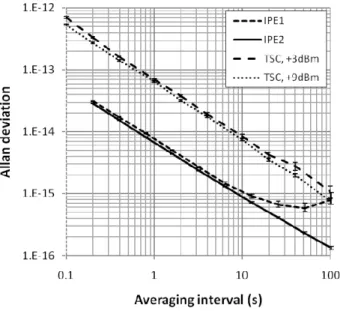
The noise performance of IPE1 and IPE2 comparators has been tested with two signals at +3 dBm power-split from the +7 dBm output of a single BVA oscillator (in the IPE1 test from oscillator D and in the IPE2 test from oscillator B). This is a common test based on the presumption that for the test signals originating from a single source we have
Pσ
y(τ) << Cσy(τ) and what we get from the test is
σy(τ) = [Cσy(τ)2 + Mσy(τ)2]1/2. To ensure sufficient rejection of
the CO noise, the test signals were set quasi-synchronous within 2x10⁻³ of the beat-note period (the same
synchronization interval was maintained during stability measurements). The results of the test are shown in Fig. 2. The increase in σy(τ) at larger τ in this specific IPE1 test is owing
to a periodic variation with a period of about 600 s whose origin is not known. Still there is no significant difference between IPE1 and IPE2 in the FFM region, i.e. in both cases the slope corresponds to flicker phase modulation (FPM) of ~7x10-15/τ which one would suppose can be neglected against
the instability of the oscillator pair.
2) Supplementary Comparator: For supplementary
measurements, we used a TSC 5110A Time Interval Analyzer serial number 129064. The 5110A analyzer provides the basic sampling interval τ0 = 10 ms though our option generates the
phase data only at 1 s intervals so the stabilities at τ < 1 s are the screen shots. The multiplication factor is 5x10⁶ at 5 MHz.
The performance test has been made under similar conditions as that of the IPE1 and IPE2 comparators and its result is also depicted in Fig. 2 along with IPE1 and IPE2. Since +3 dBm is at the TSC specification limit (+3 dBm to +17 dBm), we also tested it at a power level of +9 dBm by making use of a low-noise amplifier before the power splitter. The equivalent low-noise
Figure 2. Performance test of IPE1/IPE2 comparators and 5110A.
bandwidth (BW) of TSC is about ten times larger than that of IPE. We have verified it by measuring a 5 MHz signal with intentionally large WPM noise alternatively with IPE2 comparator and 5110A. The result was BWTSC/BWIPE = σy(τ)2TSC/σy(τ)2IPE = 10.3 in the WPM region.
C. Frequency Domain
Complementary measurements in the frequency domain have been performed with a modified Femtosecond Systems FSS1000E Phase Noise Detector [17] connected to a SR760 FFT Spectrum Analyzer. We have modified the original FSS1000E because of its poorer noise performance (larger FPM probably due to the digital potentiometer at the FSS PLL input). We have by-passed the FSS PLL circuitry with a less noisy PLL of our own design.
D. Laboratory Conditions
The laboratory for stability measurement is housed in the underground vault which ensures a stable environment, especially concerning vibrations and mechanical shocks. The room is shielded, though far from perfect. The temperature is controlled to 23 ± 1oC. During the reported measurements the
24 V DC voltage for the BVA oscillators was supplied from two Statron 2229 double AC-DC sources with 2 mV rms ripple (one Statron for A&B oscillators, the other for C&D oscillators). It should be noted that there was no other activity in the laboratory in addition to the measurement.
IV. PERFORMED MEASUREMENTS
During the campaign with four oscillators we carried out 29 measurements with the IPE1 comparator and 18 supplementary measurements with 5110A. The four oscillators formed six pairs henceforth designated as B, A-C, etc. For the stability analysis we have used the following number of measurements (in parentheses) of respective pairs: A-B (4), A-C (4), A-D (4), B-C (5), B-D (6), C-D (6) made with IPE1, and A-B (2), A-C (2), A-D (2), B-C (2), B-D (2) and C-D (8) made with 5110A. The number of samples in one
measurement series was typically 5000. It should be noted that our measurement system did not allow us to measure more than one oscillator pair at the same time.
With the reconstructed IPE2 comparator, we have made around 50 additional measurements of the A-B pair in different periods of time.
V. MEASUREMENT RESULTS
A. Measurement of A, B, C, D oscillators with IPE1
Based on the IPE1 tests, we first assumed that the impact of the measurement system was negligible, i.e. σy(τ) ≈ Pσy(τ),
and that the individual variations were uncorrelated. Under this assumption we decomposed the pair stabilities into individual stabilities with the aid of the four-cornered hat technique using two different approaches.
In the analysis reported henceforth the phase data have first been checked for outliers (actually only a few outliers have been removed). The phase data used for stability calculation are residuals of the quadratic fit. The fit removal, however, has a negligible influence on the short-term results.
1) Least-square method: To decompose the six pair
stabilities into four individual stabilities we have used the common least squares method applied to pair stabilities σy(τ)i
at all τ for all pairs. Denoting the pair stabilities as σAB(τ)i,
σAC(τ)i, σAD(τ)i, σBC(τ)i, σBD(τ)i and σCD(τ)i, and the individual
stabilities σA(τ), σB(τ), σC(τ) and σD(τ), we can form a
four-cornered hat as depicted in Fig. 3.
Figure 3. Four-cornered hat.
Based on this hat, we have for each τ an over-determined system of equations which can be solved for the individual stabilities σA(τ), σB(τ), σC(τ) and σD(τ). We can write the
equations in the form σ2 AB(τ)1 = σ2A(τ) + σ2B(τ) + ε2AB1 (5) σ2 AB(τ)2 = σ2A(τ) + σ2B(τ) + ε2AB2 … σ2 AC(τ)1 = σ2A(τ) + σ2C(τ) + ε2AC1 σ2 AC(τ)2 = σ2A(τ) + σ2C(τ) + ε2AC2 … etc.
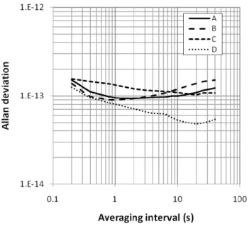
Figure 4. Individual stability from least squares decomposition.
The result of the solution is shown in the above Fig. 4. It should be noted that the use of weighted least squares has no impact on the FFM region.
2) Minimum FFM floor: This engineering approach is
based on (2). In this case we are solely interested in the FFM noise which we consider the main goal of the time-domain short-term stability measurement of this type of oscillators. We assume that for a given pair any uncorrelated stochastic variations as well as periodic fluctuations make the amount of σy(τ)i at FFM region of τ larger than the inherent FFM floor of Pσ
y(τ). Thus the minimum of all σy(τ)i, i = 1, 2, … for the
specific pair represents the best estimate of the inherent FFM floor. Clearly, we search for what we call a “justifiable” minimum which we define as σy(τ)i at τ for which we have
min [σy(τ)i + u(τ)i, i = 1, 2, …]. We have searched the minima
at 1 s < τ < 10 s. The results based on this approach are shown in Table I.
TABLE I. FFM FLOOR ESTIMATED FROM JUSTIFIABLE MINIMUM.
A B C D
Allan deviation 8.7x10⁻¹⁴ 9.4x10⁻¹⁴ 1.1x10⁻¹³ 6.0x10⁻¹⁴
B. Measurement of A,B oscillators with IPE2
Fig.5 shows the stability plots of the A-B pair obtained from the measurements with the IPE1 comparator during the campaign (thin plots), from selected measurements made with the reconstructed IPE2 comparator at a later time (bold plots), and from selected measurements performed recently with 5110A (dashed plots). The error bars are omitted for sake of clarity.
A
σA(τ)B
σB(τ) σAB(τ)iC
σC(τ) σBC(τ)i σAD(τ)iD
σD(τ) σCD(τ)i σBD(τ)i σAC(τ)iFigure 5. Frequency stability of A-B pair.
The FFM floor is about 1.3x10⁻¹³ with IPE1, 0.9x10⁻¹³ with
IPE2 and 1.5x10⁻¹³ with 5110A. Thus a significant
improvement has been observed after the reconstruction of the IPE comparator. A question arises about which of the contributions in (2) is responsible for this improvement. We can hardly expect that it has been due to improved inherent stability of the oscillators since in both measurements with IPE1 and IPE2, the oscillators had been continuously operating for a long time. Therefore we must attribute it to better performance of the measurement system, i.e. to smaller variance Cσ
y(τ)2 + Mσy(τ)2. Since we are not aware of any
changes that may have lead to significantly smaller Mσ y(τ), the
responsible contribution is most likely the inherent instability of the comparator, Cσ
y(τ). If this is true then the contribution to
the total FFM of 1.3x10⁻¹³ from the IPE1 comparator was as
large as 9x10-14. This is evidently in contradiction to what we
would expect from the IPE1/IPE2 tests which differ little giving the FPM noise of ~7x10-15/τ in the short run as shown
in Fig.2. This FPM noise is negligible against the expected FFM floor of the oscillators. This implies that the comparator performs differently with the signals from a single source (as in the test) and from two different sources (as in the stability measurement). We suspect that the CO noise is rejected differently in the two modes of measurement, based on the fact that the WPM noise in the CO used in the IPE1 comparator was about three times larger than that in the reconstructed IPE2. Actually we also suspect that this effect has manifested itself in a different manner depending on the oscillator pair. At the time of the writing this text we are not able to explain this effect.
As a result of this finding, the individual stabilities based on the measurement with IPE1 bear an unknown error because the pair stabilities that entered into the four-cornered hat were correlated. Provided that the A and B oscillators have
approximately equal inherent FFM floor (which can be deduced from the A-D and B-D pairs), the A-B pair floor of 9x10-14 found with IPE2 gives the individual floor of A and B
at a level of 6x10-14 (neglecting the contribution from IPE2
itself) which is considerably less than what we have obtained with IPE1.
C. Other Observations
1) Non-stationary background: In several measurements
performed during the campaign, we have observed non-stationary disturbing processes. Namely, at some τ the values of σy(τ)r ± ur(τ) and σy(τ)s ± us(τ), resulting from the
measurement series r and s, respectively, have given the difference |σy(τ)r – σy(τ)s| > ur(τ) + us(τ) even with the
uncertainties extended to ±3σ (99% probability).
2) Disturbing periodicity: Fig. 6 shows an uncommon
distortion of the stability plot observed in an A-D measurement series. Here the FFM floor is distorted by two periodic processes which manifest themselves in different intensity in the course of the measurement series. This effect has been detected by cutting the data into two sections. A Stable32 routine called Dynamic Stability [18], [19] is a good tool to analyze this kind of phenomena. The minimum of ~1x10-13 from the first half of data (of which, however, a
significant contribution originates from the IPE1 comparator) approximates the FFM floor of the A-D pair better than the minimum from the complete data.
3) Dispersion among measurement series: In the
measurements with IPE1, the standard deviation of σy(τ)i at
τ = 1 s is within the range 1.7x10⁻¹⁵ (pair A-D) to 5.7x10⁻¹⁵
(pair C-D). The number of measurement series is too small to draw any conclusion from this observation.
4) False phase locks: When measuring free running
highly-stable oscillators which are detuned in the order of 10-13 and which are interconnected through the measurement
system, there is always a risk for the oscillators of being pulled-in. This may end up in a false lock or just in disturbing the free-running phase. The false lock is clearly identifiable from the phase plot but it is difficult to detect a disturbing pull-in process. There are basically two ways to induce the pull-in process in these oscillators: by a reverse signal injection or through the varactor diode. Fortunately these effects are much reduced thanks to OSA’s careful design. Close inspection of the phase data of all measurement series has not revealed any false phase locks. The pull-in processes, if there are any, could not be discerned from normal noise variations.
VI. CONCLUSIONS
The measurements of the four oscillators have shown that the background instability of the comparators used, i.e. IPE1 and 5110A, was too large to be neglected. This has been found in later measurements of the two of the four oscillators performed with the reconstructed IPE2 comparator which provided better results than IPE1. Thus the results from four-cornered hat shown in Fig. 4 bear unknown errors. Therefore we plan to repeat the measurement of three oscillators (A, B and D) with the IPE2 comparator in order to determine the individual stabilities more accurately. We can conclude though that the two IPE oscillators (A and B) have the inherent FFM floor at a level of 6x10-14 and that the
FEMTO-ST oscillator (D) even has the inherent FFM floor < 6x10-14.
Our current knowledge does not allow us to explain the finding that the DMTDM comparators perform differently in the test (with signals from a single source) and in the frequency stability measurement (with signals from different sources). This effect will be further investigated. For now it is imperative for us to consider this test as “the necessary but not sufficient” condition for a good comparator performance with uncorrelated signals. The key problem of course is that we have no less noisy uncorrelated signals to test the comparator.
It should also be noted that only recently we have found that much of the IPE1 comparator inherent instability was due to mismatches of the frequency divider used after HP10811 CO (see B 1).
ACKNOWLEDGMENT
The Czech authors thank Dr. Roland Barillet of LNE-SYRTE for his help in the development of the IPE DMTDM comparator.
REFERENCES
[1] J.-P. Aubry, J. Chauvin, and F. Sthal, “A new generation of very high stability of BVA oscillators,” Proc. 21st EFTF- IEEE FCS, June 2007, in press.
[2] http://www.oscilloquartz.com/file/pdf/8600.pdf [3] http://www.oscilloquartz.com/file/pdf/8607.pdf
[4] D.W. Allan and H. Daams, “Picosecond time difference measurement system,” Proc. 29th Annu. Symp. Frequency Contr., Atlantic City, USA, pp. 404-411, 1975.
[5] S. Stein, D. Glaze, J. Levine, J. Gray, D. Hilliard, D. Howe and L.A. Erb, “Automated high-accuracy phase measurement system,” IEEE Trans. Instrum. Meas. vol. IM-32, pp. 227-231, (1983).
[6] S.R. Stein, “Frequency and time – their measurement and characterization,” in Precision Frequency Control, vol. II, E.A. Gerber and A. Ballato, Eds. New York: Academic Press, pp.229-231, (1985).
[7] L. Sze-Ming, “Influence of noise of common oscillator in dual-mixer time-difference measurement system”, IEEE Trans. on Instr. and Meas., vol. IM-35, pp. 648-651 (1986).
[8] R. Barillet, “Ultra-low noise phase comparator for future frequency standards (Comparateur de phase ultra faible bruit pour les futurs étalons de frequence),” Proc 3th EFTF, pp. 249-254, March 1989. [9] C.A. Greenhall, “Common-source phase error of a dual-mixer
stability analyzer,” TMO Progress Report 42-143, Jet Propulsion Laboratory, November 2000.
[10] G. Brida, “High resolution frequency stability measurement,” Rev. Sci. Instrum., vol. 73, pp. 2171-2174, May 2002.
[11] L. Šojdr, J. Čermák and G. Brida. “Comparison of high-precision frequency-stability measurement systems,” Proc. Joint IEEE FCS/EFTF Meeting, pp. 317-325, May 2003.
[12] L. Šojdr, J. Čermák and R. Barillet, “Optimization of dual-mixer time-difference multiplier,” Proc. 18th EFTF, CD: Session 6B/130.pdf, April 2004.
[13] D.W. Allan, “The statistics of atomic frequency standards,” Proc. IEEE, vol. 54, No. 2, pp. 221-230, February 1966.
[14] J.A. Barnes, et al, “Characterization of frequency stability,” IEEE Trans. Instrum. Meas., Vol. IM-20, No. 2, pp. 105-120, May 1971. [15] “Stable32 version 1.35: frequency stability analysis,” Hamilton
Technical Services, S. Hamilton, MA 01982 USA, (2002).
[16] W.J. Riley, “Confidence intervals and bias corrections for the Stable32 variance functions”, Hamilton Technical Services, 2000. [17] “FSS1000E Phase noise detector,” Operation Manual Rev 3.2,
Femtosecond Systems, Inc., pp.4-6, (1999).
[18] L. Galleani and P. Tavella, “The characterization of clock behavior with the dynamic Allan variance,” Proc. Joint IEEE FCS/EFTF Meeting, pp. 239-244, May 2003.
[19] L. Galleani and P. Tavella, “Tracking nonstationarities in clock noises using the dynamic Allan variance,” Proc. Joint IEEE FCS/PTTI Meeting, (2005).