HAL Id: hal-00489238
https://hal.archives-ouvertes.fr/hal-00489238
Submitted on 4 Jun 2010HAL is a multi-disciplinary open access archive for the deposit and dissemination of sci-entific research documents, whether they are pub-lished or not. The documents may come from teaching and research institutions in France or abroad, or from public or private research centers.
L’archive ouverte pluridisciplinaire HAL, est destinée au dépôt et à la diffusion de documents scientifiques de niveau recherche, publiés ou non, émanant des établissements d’enseignement et de recherche français ou étrangers, des laboratoires publics ou privés.
scheduling modeling
Olivier Henri Roux, Anne-Marie Déplanche
To cite this version:
Olivier Henri Roux, Anne-Marie Déplanche. A T-time Petri net extension for real time-task scheduling modeling. European Journal of Automation, Hermés Science, 2002, 36 (7), pp.973–987. �hal-00489238�
JESA. Volume 36 – n° 7/2002, pages 973--987
task scheduling modeling
Olivier H. Roux — Anne-Marie Déplanche
IRCCyN (Institut de Recherche en Communications et Cybernétique de Nantes) UMR CNRS 6597
Université de Nantes, Ecole Centrale de Nantes, Ecole des Mines de Nantes 1 rue de la Noë, B.P. 92101, F-44321 NANTES cedex 3
{ olivier-h.roux, anne-marie.deplanche }@irccyn.ec-nantes.fr
ABSTRACT. In order to analyze whether timing requirements of a real-time application are met, we propose an extension of the T-time Petri net model which takes into account the scheduling of the software tasks distributed over a multi-processor hardware architecture. The paper is concerned with static priority pre-emptive based scheduling. This extension consists in mapping into the Petri net model the way the different schedulers of the system activate or suspend the tasks. This relies on the introduction of two new attributes for the places (allocation and priority). First we give the formal semantics of this extended model as a timed transition system (TTS). Then we propose a method for its analysis consisting in the computation of the state class graph. Thus the verification of timing properties can be conducted (possibly together with an observator) and comes to analyze the such obtained state class graph.
R É S U M É. Dans un objectif de vérification du respect des contraintes temporelles d’exécution d’une application temps réel, nous proposons une extension des réseaux de Petri T-temporels permettant de prendre en compte l’ordonnancement des différentes entités logicielles de l’application réparties sur une architecture matérielle multi-processeurs. La politique d’ordonnancement considérée est préemptive et à priorités fixes. Cette extension consiste à projeter sur le modèle l’activation ou le blocage (par les différents ordonnanceurs du système) des entités logicielles que modélisent les places du réseau et ce, à partir de deux nouveaux paramètres (placement et priorité) associés aux places. Nous donnons dans un premier temps la sémantique formelle de ce modèle sous la forme d’un système de transitions temporisé (TTS) puis nous proposons une méthode d’analyse de ce modèle par le calcul du graphe des classes d’état. La vérification de propriétés temporelles peut alors être effectuée (avec ou non l’adjonction d’un observateur) par un examen du graphe des classes d’état ainsi obtenu.
KEYWORDS: T-time Petri net, timing analysis, static priority pre-emptive scheduling,
multi-processor real-time system, state class graph
MOTS-CLÉS : réseau de Petri T-temporel, vérification temporelle, ordonnancement
1. Introduction
1 . 1. Context of the work
An emerging stage in the development process of real-time control applications is based on the design of validated operative architecture (Durand 1998). By operative architecture, one means generally the result of the mapping of the software architecture elements onto the hardware architecture ones. Such an operative architecture has to be validated to make it possible to assert a priori that the application (timing and dependability) requirements will be met (once the detailed design and implementation have taken place). Tailored tools to support the real-time architectural design process have to be made available for the architecture designer. Our work is concerned with a particular form of this wide problem. Its main characteristics are listed hereafter :
– the software architecture is composed of a set of interacting tasks that execute applicative functions. It is static (tasks can not be created nor destructed on-line) ;
– the underlying hardware architecture is composed of multiple processors. It is static as well. The allocation of tasks to processors is known and fixed (no migration of tasks dynamically). Each processor is equipped with a dedicated operating system called executive that includes among other things a scheduler ;
– among the various scheduling techniques, the static priority pre-emptive based scheduling (at any time, among all the ready tasks, it is the one with the highest priority which runs) is commonly implemented by executives off-the-shelf. It is the scheduling strategy addressed by this work. Thus a priority is assigned to each task ;
– only timing constraints (deadline, cadence, latency, etc) on task execution are considered ;
– then, the problem to be solved is to determine a priori whether timing requirements could be missed or not due to the scheduling of tasks on the different processors.
1 . 2. Related works
Since Liu & Layland (Liu et al., 1973), the scheduling theory has received and still receives consideration, and in particular the « analytical » study of real-time task schedulability (Lehoczky et al.,1989)(Audsley et al.,1993)(Klein et al., 1993)(Tindell et al., 1993)(Palencia et al., 1998). For the most part it consists in deriving exact (necessary and sufficient conditions) or only approximate (sufficient conditions) schedulability tests, depending on the complexity of the considered model for the tasks. Thus the original configurations of independent tasks have been
extended so as to take into account shared resources, then precedence relations. Nevertheless the behavioral models for the tasks remain quite simple and do not yet support some complex synchronization schemes such as those allowed by real-time executive services. Moreover, these tests require known computation times for the tasks (often refered by WCET as “Worst Case Execution Time”). Besides the difficulty to measure or estimate such execution times, taking into consideration a fixed time (even if it is the longest) does not lead to the worst case. Actually it is easy to show that reducing the computation time of a task may surprisingly induce a decrease of timing performances for the application (Roux et al., 2001]. Moreover these approaches confine the schedulability to the sole analysis of task deadline meeting. More sophisticated timing constraints (end-to-end ones involving several interacting tasks, or cadence ones so as to bound jitter, etc) are not directly taken into account.
Consequently we have chosen to work with a more precise behavioral model for the tasks while enabling a timing labeling and a quantitative timing analysis. Different models (in most cases their structure is initially a purely behavioral one) have been modified so as to introduce time. For example, it is the case for the real-time temporal logic, a temporal extension of process algebra (known as “real-timed CCS”), the timed automata, the timed Petri nets, or the time Petri nets (Merlin, 1974). We have been interested in the latter ones. Intrinsically time Petri nets allow to model behaviors exhibiting parallelism, synchronization and sharing of resources. Moreover by allowing time specification in the form of time intervals, it is possible to express variation of processor or device performances (no determinism on task execution times is required). The structural element to which is associated the time (place, token, transition, arc) distinguishes some time sub-classes for Petri nets. It mainly gives rise to T-time Petri nets (Berthomieu et al., 1991), P-time Petri nets (Khansa, 1997), and time stream Petri nets (Diaz et al., 1994). Our study takes place in the context of T-time Petri nets.
The modeling of process scheduling with Petri nets is not well-off and has formed the subject of rare works. One can mention for example the approach of Grolleau (Choquet et al., 2000) that is based on Petri nets with a maximal firing functioning mode. The processor is modeled by a place connected by an arc to each transition of the system. The firing of a transition represents the passing of a unit of time. The goal is to extract optimal scheduling sequences from such a model. An other approach consists in modeling priorities of tasks with inhibitor arcs added to the Petri net (Robert et al., 2000). An inhibitor arc is then placed from each transition of the pattern representing a task towards each transition of the patterns representing the other lower priority tasks. In the case of timed Petri nets with inhibitor arcs, computation times are introduced through time specifications attached to transitions. Finally Okawa and Yoneda (Okawa et al., 1996) propose an approach with time Petri nets consisting in defining groups of transitions together with rates (speeds) of execution. Transition groups correspond to transitions that model
concurrent activities and that can be simultaneously ready to be fired. In this case, their rate are then divided by the sum of transition execution rates.
In our approach, we do not model explicitly the scheduling neither as an extra Petri net (that would model the computing resource, the pre-emptions or the scheduler), nor as explicit clusters. Instead the scheduling strategy is inherently included in the semantics of our model. Consequently, only the parameters that the scheduler knows are provided to the model as two parameters and this, without requiring any preliminary calculation.
1 . 3. Organization of the paper
The purpose of this paper is to present the extension we have defined for the time Petri net formalism. The remainder of the paper is organized as follows. Section 2 introduces Time Petri Nets with their scheduling extension. At first a definition is given in section 2.1 together with an intuitive then formal semantics. The computation of the marking is extended as well to the one of a new marking (we name it “active marking”) which integrates the priority based scheduling for each of the processors. In section 2.2 the properties of these “scheduling extended time Petri nets” are listed. Since timing checking requires an analysis of the modeled behaviors, we give details of the way the state class graph is computed in section 3. Section 4 offers our summary and conclusions.
2. Scheduling Extended Time Petri Nets
We propose an extension for the TPN1 that enables to take into account the way
the real-time tasks of an application distributed over different processors are scheduled. At first this extension consists in adding two parameters to the TPN’s places ; we call them “p r o c e s s o r ” and “priority”, and they correspond respectively to the allocation and the priority of the task which is associated with the place. However all places of a TPN do not require such parameters. Actually when a place does not represent a true activity for a processor (for example a register or memory state), neither a processor nor a priority have to be attached to it. In this specific case, the semantics remains unchanged with respect to a standard TPN. One can notice that it is equivalent to attach to this place a processor for its exclusive use and any priority (it does not matter in this case).
These two parameters, processor and priority, determine those transitions that are enabled and the one that is fireable from a particular state of the system. For this it is considered that there are as many schedulers as processors, and that each of them implements a priority-driven scheduling strategy. From a state, places corresponding
1. Some notations used in this paper are : - PN, for Petri Net ; - TPN, for T-time Petri Net ; - SETPN, for Scheduling Extended T-time Petri Net.
to the tasks that should be running on each processor are searched. In this way a sub-marking of the standard sub-marking is obtained that we call “active sub-marking”. Fireable transitions are looked for among those transitions that are enabled by this active marking.
2 . 1. Définition
A Scheduling Extended T-time Petri Net is a tuple : >
<
= P,T,Pre,Post,M0,I,Proc,ω,γ
R where :
– P=
{
p1,...,pm}
is a finite set of places ;– T=
{
t1,...,tn}
is a finite set of transitions ;– pre :P×T→N is the backward incidence function ; – post:P×T→N is the forward incidence function ; – M0 : P Ν is the initial marking ;
– I:T→Q≥0×(Q≥0∪∞) is the static timing function (earliest and latest firing times of transitions);
– Proc = {Proc1,….,Procr} is a finite set of processors ;
– ω : P→ N is the priority assignment function ; – γ : P→Proc∪
{ }
φ is the allocation function2.From a simple definition point of view, Proc, ω and γ are the specific elements that extend TPN to SETPN.
SOME NOTATIONS. —
– So as not to overload notations and in accordance with usual ones, we note indifferently M for the marking function M:P→N , and the marking vector
m
M∈Ν . Similarly, we note pre(t) and post(t) respectively backward incidence vector and forward incidence vector of the transition t .
– I(t)is defined as [Iα(t),Iβ(t)] where Iα(t) and Iβ(t)are respectively the earliest and latest firing times of the transition t .
– We refer to the active marking associated to the marking M by
m
) M (
act ∈Ν . It will be determined from Proc, ω et γ. We note act(M,p) the active marking of the place p.
2. The value φ is introduced so as to specify that a place is not assigned to an effective processor of the hardware architecture.
2.1.1. Unformal semantics
Main aspects of SETPN are hereafter listed in an intuitive manner.
–
ν
∈
(
R
≥0)
n is introduced as a valuation such that each νi corresponds theelapsed time while the transition t was enabled (not necessarily consecutively) byi
the active marking (act(M)≥ pre(ti)), since the last time where transition t wasi
enabled by the active marking M ≥ pre(ti).
– A transition t is fireable :i
- when it is enabled by the active marking : act(M)≥pre(ti);
- when its valuation ν ∈i [Iα(ti),Iβ(ti)] ;
- and if no other transition enabled by the active marking has to be fired before : ∀tk,
(
k≠iand (act(M)≥ pre(tk)))
⇒ν ≤k Iβ(tk)– The firing of a transition ti from a marking M gives a new marking M ’
defined by : M'=M − pre(ti)+ post(ti) 2.1.2. Formal semantics
The semantics of SETPN can be given in term of “Timed Transition Systems”(TTS) (Larsen et al., 1995) which are usual transition systems with two types of transitions : discrete transitions for events and continuous transitions for time elapsing.
We define the boolean function ↑enabled(tk,M,ti) which is true if the transition tk is newly enabled by the firing of ti and false otherwise. Formally this
gives :
(
) (
)
(
( ) ( )) (
( ) ( ) ( ))
) , ,(tk M ti ti tk M preti pretk M preti postti pretk
enabled = = ∨ − < ∧ − + ≥
↑
DE F I N I T I O N. — The semantics of a SETPN is a timed transition system
) , , ( 0 → = Q q S where : – Q Nm (R )n 0 ≥ × =
– q0 =(M0,0) ( 0 is the initial valuation ∀i∈
[ ]
1,n , 0i =0)– → ∈Q×(T∪R≥0)×Q consists of the discrete and continuous transition relations :
↑ = ∈ ∀ ∈ + − = ∧ ≥ → otherwise ), , , ( 0 ] , 1 [ ) ( ) ( ) ( ' ) ( ) ( ) ' ,' ( ) , ( ' k i k k i i i i i t t M t enabled if n k t I t post t pre M M t pre M act iff M M i ν ν ν ν ν
- the continuous transition relation is defined ∀d∈R≥0:
≤ ⇒ ≥ + ≥ ∧ ≤ = ∈ ∀ → ) ( ) ( otherwise d ), ( ) ( ) ( if ] , 1 [ ) ' , ( ) , ( ' ' ) ( i i i i i i i i d t I t pre M t pre M t pre M act n i iff M M β ε ν ν ν ν ν ν 2.1.3. Active marking ASSUMPTIONS. —
The proposed extension relies on some assumptions that are relevant to our applicative context.
– Two tasks allocated to the same processor can not have the same priority. However, the behavior of a task can be modeled by several places that inherit the same priority from it. The sequential execution of a task excludes that several places with the same priority and attached to the same processor are marked simultaneously. At the model level, it comes down to forbid SETPN for which the next property is not satisfied :
∀ p, p’∈ P2
, ( p≠p’ and γ(p)=γ(p’)≠ and M(p)≥1 and M(p’)≥1) ⇒ ω(p)≠ω(p’)φ – Furthermore synchronization between tasks are achieved by means of calls to executive services that appear explicitly while modeling the system behavior. Consequently, we assume that all direct synchronization between the models of tasks that are allocated to identical or different processors are not allowed. It can be formalized as : φ γ φ γ ≠ ⇒ = > > ∈ ∃ ∈ ∀t T,( p,p' P2,Pre(p,t) 0,Pre(p,'t) 0, (p) ) (p')
DEFINITION. — At first, for a given marking M of a SETPN, we define the set
Ema of its sub-markings : Ema = {ma1, ma2, … mas} with ∀i, mai ≤ M. An
element of Ema is called an “admissible marking”.
For the modeled application, Ema corresponds, for a given state, to the set of the
possible task activations without taking into account the scheduling algorithm. These activations are those for which : - one and only one task is being running on a
processor ; - and a task can be running if all its conditions for execution are met. The “active marking” is then the element of Ema that satisfies to the priority-based
scheduling strategy. It corresponds to the execution sequence which ensures that, for each processor, it is the ready task with highest priority that is running. It is noteworthy that the timing aspect of the SETPN is not yet taken into account in this step.
In other words, Ema is the set of the sub-markings ma of M (ma(p)=M(p) or
ma(p) =0) in which a place p is marked (ma(p)≥1) if : - p is marked in M (M ( p ) ≥ 1 ) ; - p e n a b l e s a t l e a s t o n e t r a n s i t i o n t (∃t∈T,M(p)≥Pre(p,t),Pre(p,t)>0,
(
∀p'∈P,ma(p')≥Pre(p,'t))
) ; - no other place associated with the same processor is marked in m a(∀p'∈P,
(
γ
(p)=γ
(p')≠φ
and p≠ p')
⇒ma(p')=0 ). Formally :(
)
(
)
(
)
(
)
(
)
(
)
(
)
(
)
(
)
= ⇒ ≠ ≥ ∈ ∀ > ≥ ∈ ∃ ⇒ = = ≠ ≠ ∈ ∀ ⇔ ≠ = = ⇒ = ∀ = 0 ) ( ) ( ) ( ) ,' ( )' ( , ' , 0 ) , ( ), , ( ) ( , 0 )' ( ' )' ( ) ( , ' 0 ) ( ) ( 0 ) ( 0 ) ( , / p ma p M p ma and t p Pre p ma P p t p Pre t p Pre p M T t and p ma p p and p p P p p M p ma and p ma p M p ma Ema φ γ γThe “active marking” (act(M)) is the element of Ema such that, for each of its
marked places, it does not exist an other admissible marking such that a higher priority place allocated to the same processor is marked3 there. It can be express in
the following way :
( )
(
)
(
)
(
)
( )
( )
( )
( )
(
) (
)
(
)
(
)
(
)
(
)
(
)
(
( ) ( ) 0 ( ) ( ))
' ' , ' , 0 ) ' ( / ' 0 ) ( , , , / ) ( p ma p ma p ma and p and p p or p p p p p ma P p p ma and p s i k i P p E ma M act i k i k i ma k = ⇒ > = = > = > ∈ ∃ ⇒ > ≠ ≤ ≠ ∀ ∈ ∀ ∈ = φ γ ω ω γ γ φ γPROPERTIES OF THE ACTIVE MARKING. — We have proven (Roux et al., 2001) that,
for a given marking M :
3. The consideration (in the framework of a future work) of an other scheduling strategy could consist in choosing an other element of Ema as the active marking.
– The set Ema is not empty and the null marking is always element of Ema
– There always exists an active marking act(M) (that may be the null marking). – The active marking act(M) is unique.
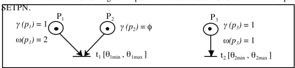
EXAMPLE. — The following example illustrates these notions with a simple
SETPN.
Figure 1. Example
From the given marking, one can find three admissible markings from which the active marking is determined :
( )
( )
{
}
( )
( )
] 0 , 1 , 1 [ ) ( ] 1 , 0 , 0 [ ], 0 , 1 , 1 [ ], 0 , 0 , 0 [ ] 1 , 1 , 1 [ 3 1 3 1 ⇒ = > = ⇒ = = M act p p Ema p p M ω ω γ γ2 . 2. Reachability and boundedness
TH E O R E M. — The reachability and boundedness problems for SETPN are
undecidable.
PROOF. — A Petri net can be expressed as a SETPN ; Petri nets are particular
cases of SETPN. Moreover a TPN can be described by a SETPN ; TPN are particular cases of SETPN. On the other hand, Menasche (Menasche, 1982) proved that Petri nets , timed Petri nets and Petri nets with inhibitor arcs can be expressed as TPN , and consequently as SETPN too. Properties of boundedness and reachability are undecidable for Petri nets with inhibitor arcs, and are therefore equally undecidable for SETPN.
However, as for TPN (Berthomieu et al., 1991), if the limits of the initial intervals of a SETPN (fixed by the static timing function) are rational numbers, and if the associated PN is bounded then the SETPN is bounded.
Outside of sufficient boundedness conditions (Berthomieu et al., 1991), only the computation of the state space allows to determine if an SETPN is bounded or not.
P3
( )
( )
1
1
3 3=
=
p
p
ω
γ
t2 [θ2min , θ2max ] P1 P2 t1 [θ1min , θ1max ] γ (p1) = 1 ω(p1) = 2 γ (p3) = 1 ω(p3) = 1 γ (p2) = φ3. State space : computation of the state class graph
TPN relying on a dense model of time, the state space is potentially infinite. Techniques for reducing the infinite state space to a finite one are necessary : several approaches have been introduced to define and compute the state class graph
(Berthomieu et al., 1991)(Boucheneb et al., 1993)(Yoneda et al., 1993) or the region graph that defines the state space too (Yoneda et al., 1998).
From now on we are interested in bounded SETPN for which we propose a technique for computing the extended state class graph inspired from (Menasche et al., 1982)(Berthomieu et al., 1991). The building of the state class graph consists in determining the set of accessible classes from a given class and repeating this operation until convergence (equality of classes) is obtained. We introduce now the specificities of the proposed extension.
– As for a TPN, the state of a SETPN is defined by a 2-uple called « class »,
(
M
D
)
C
=
,
such that :- M : P Ν is the “marking” of the class. A place p is marked if M (p)>0. M defines the set of the marked places (afterwards it will be confused with the function as well as the vector).
- D is the “firing d o m a i n ” of the class and is defined as a set of inequalities deduced from the functions α , β et δ :
+ → Q T : α ∞ ∪ →Q+ T : β ∞ ∪ → ×T Q T : δ
– The “initial state” of a SETPN is the class C =0
(
M0, D0)
where D0 is definedas :
[
]
⇒ = ∀ ∈ ≥ ∈ ∀t T, ( p P), (M0(p) Pre(p,t)) α0(t),β0(t) S(t) ∞ = ∈ ∀,' 0(,') 2 tt T t t δ– Furthermore, for each class
C
i=
(
M
i,
D
i)
of the class graph of a SETPN, we compute :- its “active marking” : act(Mi) ;
- its “active domain” : D Ai , defined in the same way as the domain Di but
restricted to those transitions that are enabled by the active marking.
– By definition, for SETPN (as for TPN), two classes C1 = (M1,D1) and C2 =
(M2,D2) are equal if and only if M1 = M2 and D1 = D2. It implies that act(M1)= act(M2
3 . 1. Active domain
Concisely we recall that the domain D of a class C = (M, D) is a system of inequalities that define the time intervals during which those transitions enabled by the marking M can be fired. These inequalities have two forms :
) ( / ) ( ) (ti ≤θi ≤β ti ∀ti M ≥pre ti α ≥ ≥ ∀ ≤ − ≤ − ) ( ) ( / , ) , ( ) , ( k j j k j k j k k j and M pret t pre M t t t t t t θ θ δ δ
where θi is the firing date of the transition ti with regard to the class C = (M,D).
The active domain DA corresponding to a class C = (M,D) is a subset of the domain D limited to the transitions enabled by the active marking. This can be expressed as shown hereafter :
≥ ≥ ∀ ← ≤ − ≤ − ≥ ∀ ← ≤ ≤ = ) ( ) ( ) ( ) ( / , ) , ( ) , ( ) ( ) ( / ) ( ) ( i j j i i j i j j i j i i i i i i t pre M act and t pre M act t t t t t t t pre M act t t t DA δ θ θ δ θ θ β θ α or more simply : ≤ − ≤ ≤ = ...... j i j i i i i DA δ θ θ β θ α
The firing space Θ (Menasche et al., 1982)(Berthomieu et al., 1991) attached to a domain DA is the set of vectors θ = (θ1 ,.. θN) solution of the inequality system that
defines DA. Its canonical form noted DA* is obtained as follows :
2
, ∈Ν
∀ ji αi* = min { θi = θ (i) | θ ∈ Θ }
βi* = max { θi = θ (i) | θ ∈ Θ }
δij* = max { θi - θj = θ (i)- θ (j) | θ ∈ Θ }
From the canonical form of the firing space DA*, it is possible to determine the
“effective upper bound” (or “UP”) which is the smallest upper bound of the inequality system that defines the canonical form of the active domain. That is to say : UP = min {βi* | i≤N}.
3 . 2. Transition firing
From a class, firing a transition gives rise to a new class for which the marking and the domain have to be determined. A class C’ = (M’,D’) reachable from a class C
= (M,D) by firing the transition ti in the interval [αi*,UP] is computed in the
following way :
– ∀p∈P, M'(p)=M(p)−Pre(p,t)+Post(p,t)
– The computation of D’ is carried out following three steps :
- 1) Remove from D the inequalities in relation with transitions that are no more enabled due to the firing of ti ;
- 2) Translate the time origin for D with αi* or UP according to the
direction of the inequality and the fact that a transition is or not enabled by the active marking act(M) : − − − ≤ − ≤ − − − − − ≤ − ≤ − − − ≤ − ≤ − − − ≤ ≤ − − + ≤ ≤ + − = ≥ ∀ < ≥ ∀ ≥ ∀ < ≥ ∀ ) , min( ) , max( ) , min( ) , max( ) , min( ) , max( ... ) , min( ) , , 0 max( ) , min( ) , , 0 max( ' ); ( ) ( / ; ) ( ) ( ), ( / ; ) ( ) ( / ; ) ( ) ( ), ( / * * * * i j k i kj j k j k jk m k km m k m k mk j l lj j l j l jl ki i k k ik k ji j j i ij j m m l l l k k j j j UP UP UP UP D t pre M act t t pre M act t pre M t t pre M act t t pre M act t pre M t α α β α δ θ θ β α δ α β δ θ θ β α δ α β δ θ θ β α δ δ α β θ δ α δ β θ α δ α
- 3) In accordance with the static timing function I, insert new equalities for those transitions that are newly enabled by M.
3 . 3. State class graph properties
Just as the class graph of a standard TPN, the class graph of a SETPN has two drawbacks : the number of classes may increase exponentially with the system size (Lilius, 1999) and the normalizing operation of the domain (canonical form) has to be conducted for each reached state ; it is a great disadvantage to its efficiency. This normalizing operation has a complexity in ( 3)
n
O , where n is the number of enabled transitions.
4. Conclusion
We have proposed an extension to T-time Petri nets allowing to take into account a pre-emptive and fixed priority based scheduling strategy. This extension allows the formal modeling of real-time processes distributed over a multi-processor hardware architecture. From bounded SETPN, the computation of the state class graph makes it possible to check timing constraints expressed as observers.
Works presented in this paper have been implemented in a tool « ROMEO » (including a graphic interface written in “tcl/tk” for editing SETPN together with a computation module written in C++ for the state class graph) (Romeo, 2001).
Our current works are concerned with the building of the SETPN state class graph as a timed automaton. That will allow to use efficient methods and tools of “model-checking” of properties expressed in temporal logic on the obtained timed automaton.
We also plan to investigate other scheduling algorithms (Round Robin, EDF, etc) either with an extension of the current analysis method, or with a structural translation of SETPN to hybrid automata.
5. References
Audsley N., Burns A., Richardson M., Tindell K., Wellings A.J., “Applying new scheduling theory to static pre-emptive scheduling”, Software Engineering Journal, september 1993, p. 284-292.
Berthomieu B., Diaz M., “Modeling and verification of time dependant systems using time Petri nets”, IEEE Transactions on Software Engineering, vol. 17, n° 3, 1991, p. 259-273.
Boucheneb H., Berthelot G., “Toward a simplified building of time Petri nets reachability graph”, 5th
international Workshop on Petri Nets and Performance Models - PNPM’P3
, Toulouse (France), october 1993, p. 46-55, n° 0-8186-4250-5/93.
Choquet-Geniet A., Grolleau E., Cottet F.,“Etude hors ligne d’une application temps réel à contraintes strictes”, Technique et Science Informatiques, vol. 19, n° 10, december 2000, p. 1373-1398, Hermès, Paris.
Diaz M., Senac P., “Time Stream Petri Nets : a model for timed multimedia information”,
1 5th
Intermantional Conference on Application and Theory of Petri Nets, Zaragosse
(Espagne), juin 1994, Lecture Notes in Computer Science, vol. 815, p. 219-238. DurandE., “Description et vérification d’architecture d’application temps réel : CLARA
et les réseaux de Petri temporels”, Ph. D. Thesis, University of Nantes, Ecole Centrale de Nantes, 1998.
Khansa W., “Réseaux de Petri p-temporels : contribution à l’étude des systèmes à évènements discrets”, Ph. D. Thesis, University of Savoie, 1997.
Klein M.H., Ralya T., Pollak B., Obenza R., Gonzalez-Harbour M. , A practitioner’s
handbook for real-time analysis : guide to rate monotonic analysis for real-time systems, Kluwer Academic Publishers, 1993, ISBN 0-7923-9361-9.
Larsen K.G., Pettersson P., Yi W., “Model-checking for real-time systems”, Lecture Notes
Lehoczky J., Sha L., Ding Y. , “The rate monotonic scheduling algorithm : exact characterization and average case behavior”, IEEE Real-Time Systems Symposium, 1989, p. 166-171.
Lilius J., “Efficient state space search for time Petri nets”, Electronic Notes in Theoretical
Computer Science, 18, 1999.
Liu C.L., Layland J.W., “Scheduling algorithms for multiprogramming in a hard real-time environment”, Journal of the ACM, vol. 20, n° 1, 1973, p. 46-61.
Menasche M., “Analyse des réseaux de Petri temporisés et application aux systèmes distribués”, Ph. D. Thesis, University Paul Sabatier, Toulouse, 1982.
Merlin P., “A study of the recoverability of computer system”, Ph.D. Thesis, Department of Computer Science, University of California, Irvine, 1974.
Okawa Y. , Yoneda T., “Schedulability verification of real-time systems with extended time Petri nets”, International Journal of Mini and Microcomputers, vol. 18, n° 3, 1996, p. 148-156.
Palencia J.C., Garcia J.J., Gonzalez-Harbour M., “Best-case analysis for improving the worst-case schedulability test for distributed hard real-time systems”, Proc. IEEE
Euromicro Real-Time Systems, 1998.
Robert P.H., Juanole G., “Modélisation et vérification de politiques d'ordonnancement de tâches temps-réel”, 8ème
Colloque Francophone sur l'Ingénierie des Protocoles -CFIP'2000, Toulouse (France), 17-20 octobre 2000, p. 167-182, Hermes.
Romeo 2001, http://www.ircyn.prd.fr/irccyn/Equipes/Temps_Reel/romeo/index.html
Roux O.H., Déplanche A.M., “Une extension des réseaux de Petri T-temporels pour la prise en compte de l’ordonnancement de tâches temps-réel dans un système multi-processeurs”, Research report, 2001, IRCCyN.
Tindell K., Clark J. “Holistic schedulability analysis for distributed hard real-time systems”, rapport de recherche n° YCS 197, 1993, Department of Computer Science, University of York.
Toussaint J., Simonot-Lion F., “Vérification formelle de propriétés temporelles d’une application distribuée temps réel”, in proceedings of Real Time System, 1997. Yoneda T., Shibayama A., Schlingloff H., Clarke E.M., “Efficient verification of parallel
real-time systems”, Lecture Notes in Computer Science, n° 697, 1993, p. 321-332. Yoneda T., Ryuba H., “CTL Model checking of time Petri nets using geometric regions”,
IEICE Transactions on Information and Systems, vol. E81-D, n° 3, 1998, p.