Wave-induced flicker level emitted by a tidal farm

HAL Id: hal-01266016

https://hal.archives-ouvertes.fr/hal-01266016

Submitted on 1 Feb 2016

HAL is a multi-disciplinary open access

archive for the deposit and dissemination of

sci-entific research documents, whether they are

pub-lished or not. The documents may come from

teaching and research institutions in France or

abroad, or from public or private research centers.

L’archive ouverte pluridisciplinaire HAL, est

destinée au dépôt et à la diffusion de documents

scientifiques de niveau recherche, publiés ou non,

émanant des établissements d’enseignement et de

recherche français ou étrangers, des laboratoires

publics ou privés.

Wave-induced flicker level emitted by a tidal farm

Anne Blavette, Bernard Multon, Hamid Ben Ahmed, Lukas Morvan, Alice

Verschae, Mohamed Machmoum, Dara O ’Sullivan

To cite this version:

Anne Blavette, Bernard Multon, Hamid Ben Ahmed, Lukas Morvan, Alice Verschae, et al..

Wave-induced flicker level emitted by a tidal farm. IEEE Power and Energy Society General Meeting (PES

GM), Jul 2015, Denver, CO, United States. �10.1109/PESGM.2015.7286290�. �hal-01266016�

Wave-induced flicker level emitted by a tidal farm

Anne Blavette

Bernard Multon

Hamid Ben Ahmed

Lukas Morvan

Alice Verschae

Mohamed Machmoum

Dara O’Sullivan

Abstract—The inherently fluctuating nature of sea waves can be reflected to a significant extent in the power output of tidal turbines. However, these fluctuations can give rise to power quality issues such as flicker. Hence, it is important to assess the impact which tidal farms may have on their local network before such power plants are allowed to connect to the grid. This paper describes the influence of the wave climate on the short-term flicker level induced by a tidal farm on the point of common coupling. It analyses also under which conditions the tidal farm breaches the grid code requirements in terms of short-term flicker level.

Index Terms—tidal energy, flicker, wave, grid code

I. INTRODUCTION

Tidal turbines are now considered as sufficiently mature to be deployed in pre-commercial tidal farms [1]-[2]. So far, they have been tested in sheltered areas where the influence of sea waves on their power output could be considered as negligible [3]. Hence, wave-induced flicker generated by tidal turbines has not been analyzed experimentally, nor has it been studied numerically, despite the significant influence waves may have on the electrical power output of a tidal turbine [4]. This paper intends to fill this gap in simulating the flicker level generated by a tidal farm by means of numerical power system simulations.

II. MODELING

A. Tidal Turbine Characteristics

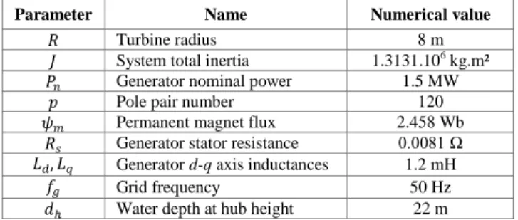
The characteristics of the tidal turbine considered in this study were extracted from [4] and are summarized in Table I. The turbine is equipped with a permanent magnet synchronous generator.

B. Modeling of the Horizontal Water Speed

The mechanical power extracted by a tidal turbine is calculated based on the horizontal component 𝑉 of the water flow speed perpendicular to the rotation plane of its blades. This horizontal speed is composed of contributions from the tidal current and from the waves. It must be noted that interactions between these two phenomena may result in a

TABLE I. TIDAL TURBINE CHARACTERISTICS

significant increase of the mean wave height [5]. However, these interactions are still not fully understood. In addition, they are currently modeled for detailed turbine structural design analyses at a relatively basic level in the ideal case of monochromatic waves superimposed to a linear tidal current [6]. Hence, it was deemed reasonable for the power system simulations performed in this study not to model these interactions at a first stage in similar fashion to [4]. Consequently, the horizontal component 𝑉 of the water flow speed at any point in space and time can be formulated as:

𝑉(𝑥, 𝑧, 𝑡) = 𝑈𝑡(𝑧, 𝑡) + 𝑈𝑤(𝑥, 𝑧, 𝑡)    where 𝑥 and 𝑧 are the horizontal and the vertical axes respectively, 𝑡 is the time, 𝑈_𝑡 and 𝑈_𝑤 are the speed contributions from the tidal current and from the waves respectively. The most unfavorable case of collinear speed contributions is considered here.

1) Tidal current contribution Ut

The tidal flow is considered as linear and perpendicular to the rotation plane (0𝑦𝑧) of the turbine blades. Hence, no turbulence effect is considered in this study. It is important to recall that, although this phenomenon may induce a significant level of flicker [3], the objective of this study consists in analyzing wave-induced flicker only.

The variation of the tidal flow speed 𝑈𝑡 at the sea surface (𝑧=0 m) as a function of time is usually considered as sinusoidal for diurnal tides such as:

Parameter Name Numerical value

𝑅 Turbine radius 8 m

𝐽 System total inertia 1.3131.106 _kg.m²

𝑃𝑛 Generator nominal power 1.5 MW

𝑝 Pole pair number 120

𝜓𝑚 Permanent magnet flux 2.458 Wb

𝑅𝑠 Generator stator resistance 0.0081 Ω

𝐿𝑑, 𝐿𝑞 Generator d-q axis inductances 1.2 mH

𝑓𝑔 Grid frequency 50 Hz

𝑈𝑡(0, 𝑡) = 𝑈𝑡,𝑚𝑎𝑥sin (2𝜋𝑡_𝑇

𝑡) 

where 𝑈_{𝑡,𝑚𝑎𝑥} is the maximum tidal current speed selected arbitrarily as equal to 3.5 m/s in this study. This value is typical of high speed tidal currents characterizing the areas where tidal farms are envisaged to be deployed. Term 𝑇𝑡 is the tidal period almost equal to half a lunar day, i.e. 12h25 ≈ 44,700 seconds. The variations of the tidal flow speed as a function of the water depth 𝑧 (𝑧 < 0) for a given time 𝑡0, can be modeled as follows [7]:

𝑈𝑡(𝑧, 𝑡0) = 𝑈𝑡(0, 𝑡0) (𝑑+𝑧_𝑑 ) 1/7

 

where 𝑑 is the distance between the sea surface and the sea bottom which is equal to 35 m in this study. This water depth corresponds to this of the site selected for the Paimpol-Bréhat tidal farm in France [4]. In summary, the contribution in speed 𝑈𝑡 from the tidal current can be expressed as:

𝑈𝑡(𝑧, 𝑡) = 𝑈𝑡,𝑚𝑎𝑥sin (2𝜋𝑡_𝑇 𝑡) ( 𝑑+𝑧 𝑑 ) 1/7 (4) 2) Waves contribution Uw

Sea surface elevation is usually modeled using linear wave theory [8]. However, this theory is not valid for shallow to intermediate waters which are traditionally characterized by a water depth less than 50 m, as it is the case in this study. Stokes’ wave theory is the typical alternative for modeling non-linear waves in shallow to intermediate waters. The order of Stokes’ law must be selected based on the wave climate characteristics considered, i.e. the significant wave height 𝐻𝑠 and the peak period 𝑇𝑝, and on the water depth 𝑑. The significant wave height 𝐻𝑠 is the height of the one-third of the highest waves of a sea-state and the peak period 𝑇_𝑝 is the period corresponding to the frequency band Δ𝑓 with the maximum value of spectral density in the non-directional wave spectrum 𝑆(𝑓) characterizing a given sea-state. A classical Bretschneider spectrum was selected. It is defined as [8]: 𝑆(𝑓) = 5𝐻𝑠2 16𝑇_𝑝4 1 𝑓5𝑒 − 5 4𝑇𝑝4𝑓 ₍₅₎

In this study, the significant wave height range considered is 2 m ≤ 𝐻𝑠 ≤8 m and the peak period range considered is 5 s ≤ 𝑇𝑝 ≤15 s. These values correspond to wave climates having low to high energy levels.

It appears clearly from Fig. 1 that the waves can be modelled as 2nd order Stokes waves for the cases considered in this study. In the case of a monochromatic wave of height 𝐻 and of period 𝑇, the velocity potential 𝜙 can thus be expressed as [10]: 𝜙 =𝐻𝐿 2𝑇 𝑐ℎ(𝑘(𝑑 + 𝑧)) 𝑠ℎ(𝑘𝑑) sin(𝑘𝑥 − 𝜔𝑡) +3𝜋 2_𝐻2 16𝑇 𝑐ℎ(2𝑘(𝑑 + 𝑧)) 𝑠ℎ4_(𝑘𝑑) sin(2(𝑘𝑥 − 𝜔𝑡)) (6)

Figure 1. Domains of validity of several wave theories (after [9]) where 𝑘 is the wave number defined as 𝑘 = 2𝜋/𝐿 = 𝜔/√𝑔𝑑 [8] 𝜔 the radian frequency defined as 𝜔 = 2𝜋𝑓. Hence, the contribution in speed 𝑈_𝑤𝑖 on the 𝑥 (horizontal) axis from a single monochromatic wave can be calculated as:

𝑈𝑤_𝑖(𝑥, 𝑧, 𝑡) = 𝜕𝜙 𝜕𝑥 = 𝜋𝐻 𝑇 𝑐ℎ(𝑘(𝑑 + 𝑧)) 𝑠ℎ(𝑘𝑑) cos(𝑘𝑥 − 𝜔𝑡) +3𝜋 2_𝐻2 4𝑇𝐿 𝑐ℎ(2𝑘(𝑑 + 𝑧)) 𝑠ℎ4_(𝑘𝑑) cos(2(𝑘𝑥 − 𝜔𝑡)) (7) However, a sea-state is the sum of multiple waves of amplitude 𝑎𝑖, of period 𝑇𝑖 and of wave number 𝑘𝑖. Hence, the total contribution in speed 𝑈𝑤 of all the monochromatic waves is the sum of their individual contributions 𝑈𝑤_𝑖 such as: 𝑈𝑤(𝑥, 𝑧, 𝑡) = ∑ 𝑈𝑤_𝑖(𝑥, 𝑧, 𝑡) 𝑖 = ∑ 2𝜋𝑎𝑖 𝑇𝑖 𝑖 𝑐ℎ(𝑘𝑖(𝑑 + 𝑧)) 𝑠ℎ(𝑘𝑖𝑑) cos(𝑘𝑖𝑥 − 𝜔𝑖𝑡) +3𝜋 2_𝑎 𝑖2 𝑇𝑖𝐿𝑖 𝑐ℎ(2𝑘𝑖(𝑑 + 𝑧)) 𝑠ℎ4_(𝑘 𝑖𝑑) cos(2(𝑘𝑖𝑥 − 𝜔𝑖𝑡)) (8)

The amplitudes 𝑎𝑖 are calculated such as [8]:

𝑎𝑖= √2𝑆(𝑓𝑖)Δ𝑓 (9) 3) Averaged water flow speed

As it will be explained in the next section, the mechanical power extracted by the tidal turbine depends on the cube of the water flow speed 𝑉(𝑡)̅̅̅̅̅̅ averaged over the circular surface swept by the blades. This variable can be calculated as:

𝑉(𝑡)

̅̅̅̅̅̅ =∫_{−𝑑ℎ−𝑅}−𝑑ℎ+𝑅 𝑉(𝑥,𝑧,𝑡)2√𝑅2−(𝑑ℎ+𝑧)2𝑑𝑧

π𝑅2 (10)

Profiles for the average speed 𝑉(𝑡)̅̅̅̅̅̅ were simulated for four values of the significant wave height 𝐻𝑠: 2 m, 4 m, 6 m, 8 m,

Figure 2. Power coefficient 𝐶𝑝 as a function of the tip speed ratio λ

and for four values of the peak period 𝑇𝑝: 5 s, 7 s, 9 s, 11 s, 13 s, 15 s.

C. Modeling of the Tidal Turbine

The mechanical power 𝑃𝑚𝑒𝑐 extracted by the tidal turbine can be expressed as:

𝑃𝑚𝑒𝑐(𝑡) =1₂𝜌𝜋𝑅2𝐶𝑝(𝑉(𝑡)̅̅̅̅̅̅) 3

(11)

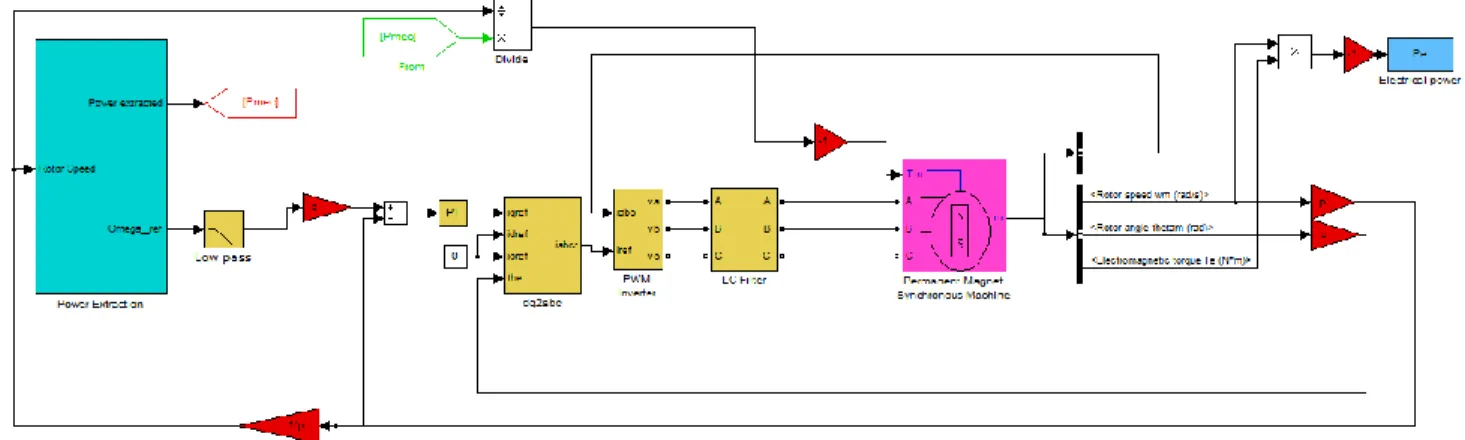
where ρ is the density of sea water equal to 1027 kg/L and 𝐶𝑝 is the power coefficient. The curve of the optimal power coefficient 𝐶𝑝 as a function of the tip speed ratio λ considered in this study was extracted from [4] and is reproduced in Fig. 2. The tidal turbine is controlled in speed so that the power coefficient 𝐶𝑝 remains sufficiently close to its maximal value. The control system was developed under Matlab- Simulink and is shown in Fig. 3. The mechanical power 𝑃𝑚𝑒𝑐 extracted by the tidal turbine is computed based on the rotor speed and on the 𝐶𝑝-λ characteristic of the turbine in the “Power extraction” block. This block computes also the dynamic reference speed ω𝑟𝑒𝑓(𝑡) to maintain power coefficient 𝐶𝑝 close to its maximal value. The error between the dynamic reference speed ω_𝑟𝑒𝑓(𝑡) and the rotor speed is transformed into phase voltages to be applied at the terminals of the turbine. The blocks “dq2abc” and “PWM inverter” were extracted from Simulink model “power_pmmotor.mdl” which simulates field-oriented control [11]. The d-q axes inductances 𝐿𝑑 and 𝐿𝑞 are equal and the generator has permanent magnet excitation so the control of the electrical torque 𝑇𝑒 relies solely on the quadrature axis current 𝑖𝑞. The direct axis current 𝑖𝑑 is maintained at zero.

D. Modeling of the Tidal Farm

The electrical power output 𝑃𝑡𝑜𝑡 of an entire tidal farm composed of 20 turbines was simulated based on the addition of identical individual electrical power profiles 𝑃_𝑒𝑛 (where 𝑛=[1, …, 20]) each shifted by a random time delay δ𝑛. The tidal turbines are assumed to be operated at unity power factor, thus leading to a farm nominal power 𝑆_𝑛 equal to 20×1.5=30 MVA.

E. Modeling of the Electrical Network

The electrical network was modeled under power system simulator PowerFactory [12] as shown in Fig. 4. It is composed of (from right to left): a “static generator” built-in model outputting the electrical power output 𝑃𝑡𝑜𝑡 of the tidal farm, a 0.4/10 kV transformer, a 1 km long submarine cable whose length was selected arbitrarily, a 0.1 MVA load (load 1), a 5 km long overhead line, a VAr compensator to maintain the power factor at the point of common coupling (PCC) at unity, a 20/38 kV transformer, a 2 MVA load (load 2) and finally a 15 Ω impedance in series with a constant 38 kV voltage source simulating the rest of the national grid. This model is inspired from a model already used in previous works [13] and representing the Irish marine energy test site, called AMETS, located off Belmullet [14]. Short-term flicker was evaluated by means of a flickermeter compliant with IEC standard 61000-4-15 [15].

III. RESULTS

A. Influence of the Wave Climate on the Flicker Level 1) Significant wave height 𝐻𝑠

Fig. 5 presents the flicker level 𝑃𝑠𝑡 as a function of significant wave height 𝐻𝑠 for different impedance angles Ψk and different peak periods 𝑇𝑝. It appears clearly that the significant wave height 𝐻𝑠 has a considerable influence on the flicker level 𝑃𝑠𝑡. However, this influence is highly dependent on the impedance angle Ψ_k. This can be explained by means of the simple two-bus system shown in Fig. 6. The generator G connected to Bus 1 injects a complex power 𝑃 + 𝑗𝑄 (where 𝑗 is the imaginary unit) into to the impedance

Figure 4. Electrical network modeled under PowerFactory

Figure 5. Flicker level 𝑃𝑠𝑡 as a function of significant wave height 𝐻𝑠 for

different impedance angles Ψ𝑘 and different peak periods 𝑇𝑝

𝑅𝑒𝑞+ 𝑗𝑋𝑒𝑞 connected in series with a constant voltage source simulating an infinite grid. The energy transport results in both active and reactive power consumption in the impedance which increases with the amount of active power 𝑃 injected. Hence, the impedance acts as a load. Its reactive power consumption is supplied by the constant voltage source which acts as a slack bus. This case can be approximated qualitatively to the classic two-bus system connected by a lossless line, provided that the active and reactive power consumption of the impedance is transferred to generator G. In this case, the voltage deviation 𝛥𝑉 = 𝑉1− 𝑉2 can be formulated as:

Δ𝑉 =𝑃𝑅𝑒𝑞+𝑄𝑋𝑒𝑞

𝑉1 (12)

Hence, for sufficiently low impedance angles Ψ𝑘 (i.e. resistive networks), the voltage deviation Δ𝑉 is influenced mostly by the active power 𝑃. On the contrary, for sufficiently high impedance angles Ψ_k (i.e. reactive networks), the influence of the reactive power 𝑄 dominates.

Figure 6. Simple two-bus system

In similar fashion, the influence of the active power 𝑃_𝑡𝑜𝑡 generated by the farm decreases as a function of the impedance angle Ψ_k, as it is more and more reduced by the opposite influence of the reactive power flow to the series reactor, the 20/38 kV transformer and the 38kV load. Hence, the amplitude of the voltage variations initially induced by the tidal farm decreases up to Ψk=70°, thus resulting in a lower flicker level. However, the influence of the reactive power flow is predominant for Ψ_k=85°, which leads to an increase of the voltage fluctuations amplitude, thus to a higher flicker level.

2) Peak period Tp

It can be observed from Fig. 5 that the peak period 𝑇𝑝 has a non-negligible, though more limited influence on the flicker level 𝑃_𝑠𝑡 than the significant wave height 𝐻_𝑠. However, as it can be observed in Fig. 6, there is no trivial relation between the flicker level 𝑃_𝑠𝑡 and the peak period 𝑇_𝑝. This was expected due to the low level of coupling between the speed fluctuations induced by the waves and the individual electrical power output 𝑃𝑒 of each turbine due to their large inertia 𝐽. In a previous work focusing on wave energy devices [16], it had been demonstrated that the flicker level induced by a wave farm including no means of storage could be reasonably well estimated by means of a sinusoidal voltage profile whose period was equal to the sea-state energy period (which is proportional to the peak period 𝑇_𝑝 used here). However, this method was no longer applicable in the case where a significant storage capacity was included in the wave farm. In similar fashion, the large inertia of tidal turbines acts as a storage means of considerable energy capacity.

B. Compliance of the tidal farm with flicker requirements In order to maintain the quality of the electricity supplied to the customer, grid operators require that any grid-connected installation complies with a certain number of requirements, and among them flicker requirements. In most grid codes, flicker is required to be maintained under a maximal allowed limit at the PCC. Numerical values found in a number of national grid codes range between 0.35 and 1 for short-term flicker [13]. In order to perform an analysis independent of the short-circuit level 𝑆_𝑘 of the rest of the national grid, the flicker coefficient 𝑐𝑓(Ψk) was used. This

coefficient is expressed as [17]:

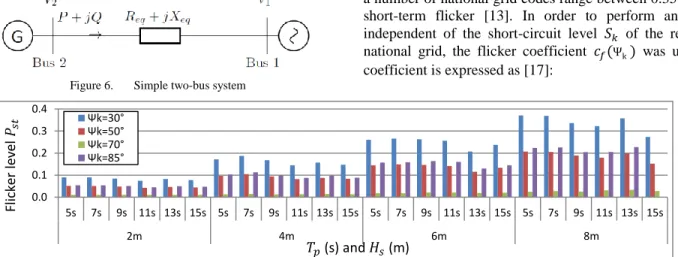
Figure 7. Flicker level 𝑃𝑠𝑡 as a function of the peak period 𝑇𝑝 and of the significant wave height 𝐻𝑠 for different impedance angles Ψk

0.0 0.1 0.2 0.3 0.4 0 2 4 6 8 10 Ψk=30° Ψk=50° Ψk=70° Ψk=85° Fl ic ke r le ve l 𝑃 𝑠𝑡 𝐻𝑠 (m) 0.0 0.1 0.2 0.3 0.4 5s 7s 9s 11s 13s 15s 5s 7s 9s 11s 13s 15s 5s 7s 9s 11s 13s 15s 5s 7s 9s 11s 13s 15s 2m 4m 6m 8m Ψk=30° Ψk=50° Ψk=70° Ψk=85° Fli cker le ve l 𝑃𝑠𝑡 𝑇𝑝 (s) and 𝐻𝑠 (m)

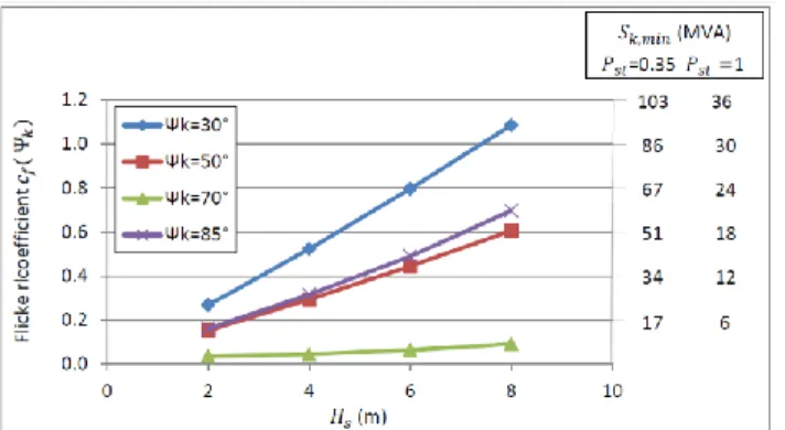
Figure 8. Flicker level 𝑃_𝑠𝑡 as a function of the peak period 𝑇_𝑝 𝑐𝑓(Ψk) = 𝑃𝑠𝑡𝑆_𝑆𝑘

𝑛 (13)

For a given impedance angle Ψ_k, the flicker coefficient 𝑐𝑓(Ψk) is constant. Fig. 8 shows the flicker coefficient

𝑐𝑓(Ψk) as a function of the significant wave height 𝐻𝑠 for different impedance angles Ψ_k. The minimum short-circuit level 𝑆_{𝑘,𝑚𝑖𝑛} for which the flicker level 𝑃_𝑠𝑡 remains below the maximum allowed flicker level limit 𝑃_{𝑠𝑡,𝑚𝑎𝑥} is calculated such as:

𝑆𝑘,𝑚𝑖𝑛=

𝑐_𝑓(Ψk )𝑆𝑛

𝑃𝑠𝑡,𝑚𝑎𝑥 (14)

Numerical values of the minimum short-circuit level 𝑆𝑘,𝑚𝑖𝑛 are shown on the right-hand side of Fig. 8. They correspond to the values of the flicker coefficient 𝑐𝑓(Ψk )

indicated on the left-hand side axis of the graph. The values for 𝑆𝑘,𝑚𝑖𝑛 were calculated for each of the maximum allowed flicker limits considered in this study and equal to 0.35 and 1.0 respectively. It can be observed that the minimum short-circuit level 𝑆_{𝑘,𝑚𝑖𝑛} for which the flicker level 𝑃_𝑠𝑡 remains below unity is relatively close to the nominal power of the tidal farm. Considering that it is unlikely that a 30 MW tidal farm may be envisaged to be connected to such nodes due to power transmission capacity issues, the flicker level 𝑃𝑠𝑡 can be considered as unlikely to exceed the most permissive limit. The same observations apply to most situations in the case of the most stringent flicker limit equal to 0.35. However, this limit may be exceeded in the rare cases meeting the three following conditions: 1) the tidal farm is connected to a node of relatively low short-circuit level in the range of approximately 50 MVA to 100 MVA, 2) the tidal farm is operated in highly energetic wave conditions (𝐻𝑠≥6 m), which is quite unlikely, 3) the impedance angle Ψk of the grid node to which the tidal farm is connected is less than or equal to 50°, or equal to 85°. Hence, based on these observations, it can be concluded that the flicker level induced by a tidal farm on its local network is unlikely to exceed even the most stringent flicker limit. It is important to point out that the influence of no other storage means (e.g. batteries, supercapacitors) than the tidal turbine inertia was included in the model. However, this study has also shown that flicker could reach significant levels. This could contribute to make the total flicker level induced by the tidal farm and other installations connected to the same node exceed the

maximum allowed limit in the case where the pre-connection flicker is already significantly high.

IV. CONCLUSIONS

This paper has described the influence of sea waves on the quality of the electrical power output generated by a tidal farm in terms of short-term flicker level 𝑃𝑠𝑡. First, the influence of the wave climate characteristics (significant wave height 𝐻𝑠 and peak period 𝑇𝑝) on the flicker level 𝑃𝑠𝑡 was studied. Then, the compliance of the tidal farm with the grid code requirements in terms of short-term flicker level was also analyzed in the second part of this paper. It was shown that the flicker level 𝑃𝑠𝑡 induced by the tidal farm at the point of common coupling is unlikely to exceed even the most stringent limit found among a number of national grid codes. However, the flicker induced by the tidal farm reaches significant levels. Hence, in the case where the pre-connection flicker level is already significant, the grid connection of a tidal farm may lead the total flicker level at the point of common coupling to exceed the maximum allowed limit.

REFERENCES

[1] EDF, Tidal farm of Paimpol-Bréhat, France, http://energie.edf.com

[2] RITE project, Verdant Power, http://www.verdantpower.com

[3] J. MacEnri, M. Reed, and T. Thiringer, “Influence of tidal parameters on SeaGen flicker performance”, Phil. Trans. R. Soc. A, vol. 371, no. 1985, February 2013.

[4] Z. Zhou, F. Scuiller, J. Charpentier, M. El Hachemi Benbouzid and T. Tang, “Power Smoothing Control in a Grid-Connected Marine Current Turbine System for Compensating Swell Effect”, IEEE

Trans. on Sustainable Energy, vol. 4, pp. 816-826, July 2013.

[5] A. Saruwatari, D. Ingram and L. Cradden, “Wave-current interaction effects on marine energy converters”, Ocean

Engineering, vol. 73, pp. 106-118, 2013.

[6] P. Galloway, L. Myers, A. Bahaj, “Quantifying wave and yaw effects on a scale tidal stream turbine”, Renewable Energy, vol. 63, pp. 297- 307, 2014.

[7] B. Multon, Marine Renewable Energy Handbook, Wiley, 2013. [8] J. Falnes, Ocean Waves and Oscillating Systems: Linear

Interactions Including Wave-Energy Extraction, Cambridge

University Press, 2002.

[9] B. Le Méhauté, An Introduction to Hydrodyanmics and Water

Waves, Berlin: Springer-Verlag, 1976.

[10] M. Brorsen, “Non-linear Waves”, Lecture notes, Aalborg University, 2007.

[11] L.-A. Dessaint and R. Champagne, “Permanent Magnet Synchronous Machine”, Matlab-Simulink model, R2014b. [12] DIgSILENT PowerFactory, http://www.digsilent.de/

[13] A. Blavette, D. O’Sullivan, R. Alcorn, T. Lewis and M. Egan, “Impact of a Medium-Size Wave Farm on Grids of Different Strength Levels”, IEEE Trans. on Power Systems, vol. 29, pp. 917 – 923, March 2014.

[14] AMETS test site, www.seai.ie, accessed on 2014/11/21.

[15] IEC Flickermeter - Functional and design specifications, standard

61000-4-15, ed2.0, 2010.

[16] A. Blavette, R. Alcorn, M. Egan, D. O’Sullivan, M. Machmoum and T. Lewis, “A novel method for estimating the flicker level generated by a wave energy farm composed of devices operated in variable speed mode”, in Proc. Int. Conf. EVER14, Monaco, March 2014. [17] IEC Measurement and assessment of power quality characteristics