HAL Id: hal-03124796
https://hal.archives-ouvertes.fr/hal-03124796
Submitted on 29 Jan 2021
HAL is a multi-disciplinary open access
archive for the deposit and dissemination of
sci-entific research documents, whether they are
pub-L’archive ouverte pluridisciplinaire HAL, est
destinée au dépôt et à la diffusion de documents
scientifiques de niveau recherche, publiés ou non,
Evidence of residual ferroelectric contribution in
antiferroelectric lead-zirconate thin films by first-order
reversal curves
Kevin Nadaud, Caroline Borderon, Raphaël Renoud, Micka Bah, Stephane
Ginestar, Hartmut Gundel
To cite this version:
Kevin Nadaud, Caroline Borderon, Raphaël Renoud, Micka Bah, Stephane Ginestar, et al..
Evi-dence of residual ferroelectric contribution in antiferroelectric lead-zirconate thin films by first-order
reversal curves. Applied Physics Letters, American Institute of Physics, 2021, 118 (4), pp.042902.
�10.1063/5.0043293�. �hal-03124796�
AIP/123-QED
Evidence of residual ferroelectric contribution in anti-ferroelectric lead-zirconate thin films by First-Order Reversal Curves
Kevin Nadaud,1,a)Caroline Borderon,2,b)Raphaël Renoud,2
Micka Bah,1
Stephane Ginestar,2and Hartmut W. Gundel2
1)GREMAN UMR 7347, Université de Tours, CNRS, INSA-CVL,
16 rue Pierre et Marie Curie, 37071 Tours, France
2)IETR, UMR CNRS 6164, Université de Nantes, 44322 Nantes,
France
In this study, two different methods have been used in order to characterize lead-zirconate anti-ferroelectric thin film elaborated by a modified sol-gel process: First-Order Reversal Curves (FORC) measurements and impedance spectroscopy coupled to hyperbolic law analysis. Approaches at low and high applied electric fields allow concluding on the presence of a weak residual ferroelectric behavior even if this con-tribution is not visible on the polarization-electric field loops. Moreover, the weak ferroelectric phase seems to switch only when the phase of the antiferroelectric cells is modified and no coalescence of ferroelectric domains at low field occurs due to a well distribution of small residual ferroelectric clusters in the material. The main goal of this paper is to show that FORC distribution measurements and impedance spec-troscopy coupled to the hyperbolic law analysis are very sensitive and complementary methods.
Keywords: Anti-ferroelectric, domain walls, hyperbolic law, FORC distribution, residual-ferroelectricity
a)Author to whom correspondence should be addressed:kevin.nadaud@univ-tours.fr b)Electronic mail:caroline.borderon@univ-nantes.fr
1
Antiferroelectric materials already have shown interest for various electronic applications such as energy storage supercapacitors1,2, pyroelectric sensors3or piezoelectric transducers2. These materials are closely related to ferroelectric thin films where interest has been found due to their high-k character and due to their tunable permittivity under a DC electric field EDC. More recently, antiferroelectrics have attracted interest for the capability to realize
non-volatile data storage components4 and their negative capacitance behavior might be used for low power electronics5.
Modeling of the material’s electrical behavior allows better understanding of the under-lying physical phenomena. However, due to its nonlinear behavior, conventional impedance spectroscopy is not sufficient for a complete description of an antiferroelectric material and thus Rayleigh analysis has been developed. Other specific characterization methods, like do-main wall motions measurements or First-Order Reversal Curves (FORC), may also be used. The FORC method has been initially used in order to obtain the Preisach density of ferro-magnetic material6,7but it has been also successfully adapted to ferroelectric material8–11. This method allows decomposition of the full polarization loop P (E) into elementary hys-teresis elements, so-called hysteron, and provides information on fatigue and degradation of the ferroelectric polarization9,12–14. It is also possible to determine the presence of a parasitic phase in magnetic material15,16.
The FORC experimental determination is done by measuring the polarization as a func-tion of the electric field using a bipolar signal with an increasing magnitude, as suggested by Cima et al17. This method allows reconstruction of the FORC distribution in two parts. The bottom triangle, delimited by (E, Er) = (0, 0), (+Emax, −Emax) and (−Emax, −Emax),
is computed using the polarization with an increasing electric field. The right triangle, de-limited by (E, Er) = (0, 0), (+Emax, −Emax) and (+Emax, +Emax), is computed using the
polarization with a decreasing electric field. For the bottom triangle, the initial field is called Er and the polarization is measured as a function of the field E (sometimes noted β and
α respectively9,12,18). The measured polarization for this curve is noted P−(E
r, E). The
measurement is repeated with a ever higher maximum magnitude of the electric field until saturation. The FORC distribution is defined as the mixed second derivative:
ρ−(E r, E) = 1 2 ∂2P−(Er, E) ∂Er∂E , (1)
which corresponds also to the variation of the differential susceptibility when Erchanges: ρ−(E r, E) = 1 2 ∂χ−(E r, E) ∂Er . (2)
A large variation of the susceptibility, when the initial field goes from Er to Er+ ∆Er in
a given range of field [E, E + ∆E], indicates a large number of cells which have a back-switching field between Erand Er+ ∆Er and a switching field in the interval [E, E + ∆E].
A large value of the FORC distribution is thus obtained in this area. A similar procedure is used in order to fill the right triangle of the FORC diagram using the decreasing part of the P (E) loops.
In this paper, the presence of a residual ferroelectric phase in an antiferroelectric thin film of PbZrO3(PZO) is studied using the FORC measurement. The presence of this ferroelectric
behavior is then confirmed by measuring the relative permittivity as a function of the AC-driving field in order to show a Rayleigh behavior corresponding to ferroelectric domain wall motions12,18,19. Subsequently, vibration and pinning of those domain walls are studied using the hyperbolic law20,21. The residual ferroelectricity in PZO has already been shown using this law22but FORC measurement has not been used on antiferroelectric materials for the study of a possible ferroelectric behavior. Moreover, in this paper, the AC field used for the hyperbolic analysis is higher than the one reported in the literature, which allows to see the limit of the Rayleigh region.
The PbZrO3thin films were elaborated by a sol-gel process and the details are reported
elsewhere22. The obtained solution is deposited on alumina substrates (precoated with a titanium interface layer and the platinum bottom electrode) at 4000 rpm during 25 s using a multi-step spin coating process. Each PZO layer is annealed during 10 min in a pre-heated open air furnace at 650◦C in order to obtain the crystalline perovskite structure. The
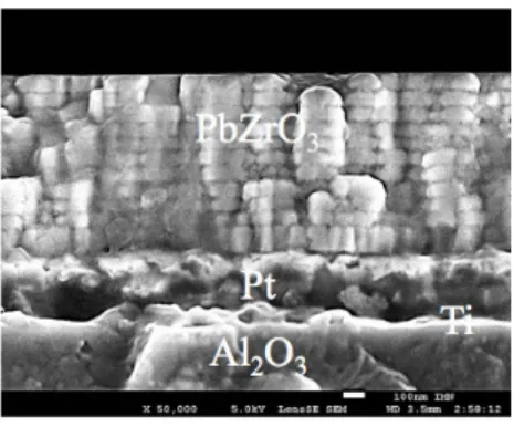
cross-section image of the PbZrO3/Pt/Ti/Al2O3 samples (obtained with a Jeol 7600 scanning
electron microscope) is shown in Fig. 1. The PbZrO3 films have an uniform, dense and
void-free microstructure without cracks and are composed of a columnar structure. The interfaces between the individual PZO layers, of approximately 70 nm thickness, are well visible and the overall film thickness for a 12 layers film is 800 nm.
Square platinum electrodes of 0.1 mm width are deposited on the top of the PZO films by RF magnetron sputtering in order to realize a Metal-Insulator-Metal (MIM) capacitor together with the platinum bottom electrode for the dielectric characterizations of the
fabri-3
Figure 1. Cross-section SEM image of the PbZrO3/Pt/Ti/Al2O3sample
cated thin films. The real and the imaginary parts of the relative permittivity are calculated from the measured capacitance and the dielectric losses (tan δ) using the well-known parallel plate expression:
C = ε0ε′r
S
t, (3)
with ε0 = 8.85 × 10⁻¹²F/m the vacuum permittivity, ε′r the relative permittivity of the
material, S the area of the electrode and t the thickness of the material.
The measurements have been performed with a AixACCT TF2000 ferroelectric analyzer at 1 kHz and custom scripts have been used in order to allow automatic data analysis. The complex electric impedance of the sample has been extracted from the applied voltage and the measured current: (i) its modulus is the ratio between the voltage and the current modulus and (ii) its angle is the phase shift between the voltage and the current.
The polarization has been obtained by integrating the current over the time, which is done by the software of the TF2000 analyzer. This method is applicable since the leakage current of the sample is considered to be negligible. The FORC distribution has been measured by applying a positive voltage in order to saturate the material and recording the polarization while decreasing the electric field and going back to the saturation field. A maximum voltage of 70 V and step voltage of 1 V have been chosen, which correspond to a maximum field of 875 kV/cm and a step field of 12.5 kV/cm representing the resolution of the distribution. The FORC distribution has been measured with a slew rate of 1 V/ms.
The P (E) loops of the lead zirconate thin films which were used for the extraction of the FORC distribution are shown in Fig.2a. The PZO presents a double hysteresis loop,
indicating its antiferroelectric nature and has a slim hysteresis loop characteristic of low dielectric losses. The maximum value of polarization is 25.5 µC/cm2which is close to the
value reported elsewhere23. The antiferroelectric to ferroelectric and ferroelectric to antifer-roelectric transition fields are respectively E+
AF= 690 kV/cm and EFA+ = 300 kV/cm for the
positive field and E−
AF = −600 kV/cm and EFA− = −330 kV/cm for the negative field. From
the P (E) loops no ferroelectric phase can be discerned.
The FORC distribution corresponding to the P (E) loop is shown in Fig.2b. Two peaks at positions (E, Er) =(−340 kV/cm, −630 kV/cm) and (705 kV/cm, 330 kV/cm) are visible
corresponding to the antiferroelectric behavior. The two maxima are not exactly symmetri-cal to the Er= −E axis which can be attributed to an internal field. The fields found from
the FORC measurements are in good agreement with the E+AF, E
+
FA, EAF− , EFA− transition
fields determined with the P (E) loops measurement. In addition to the two antiferro-electric maxima, a less pronounced peak is visible at (E, Er) = (620 kV/cm, −585 kV/cm)
which corresponds to a small ferroelectric switching polarization. The FORC measurement hence allows to state that the remanent polarization at zero electric field observed on the P (E) major loop corresponds to a ferroelectric contribution and not to dielectric losses, also broadening the P (E) loop and leading to misinterpretations24,25. This low proportion of ferroelectric domains switch for a field corresponding to E+
AF and EAF− suggesting that the
switching can occur only when antiferroelectric cells modify their phase. Residual ferroelec-tricity into antiferroelectric materials has already been investigated using P (E) loops but in the case of low applied electric fields26–28, for different sample thicknesses23or for another compound using Rayleigh analysis29. Before and after FORC distribution measurement, P (E) loops have been measured and there is no visible difference indicating the material is in the same state (results presented in supplementary material).
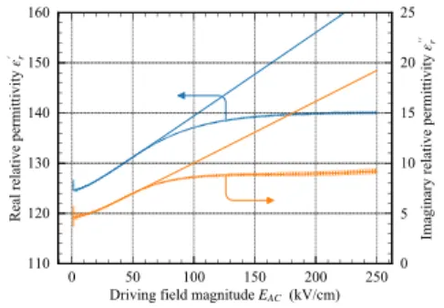
The real and imaginary parts of the permittivity as a function of the magnitude of the driving field EAC are shown in Fig.3. In order to verify the presence of the ferroelectric
phase, impedance spectroscopy has been carried allowing to see a possible increase of the permittivity when the driving electric field increases19,20. Only ferroelectric domain walls contribute to this increase since antiferroelectric domain wall motion cannot appear under the action of an homogeneous electric field30. The ferroelectric behavior is well visible since the increase on the real part of the permittivity is 9.5 %, when the electric driving field goes from 10 kV/cm to 100 kV/cm. A more important increase of the imaginary part of the
5
30 20 10 0 10 20 30 P (µ C/ cm 2) (a) 750 500 250 0 250 500 750 E (kV/cm) 750 500 250 0 250 500 750 Er (kV /cm ) (b) (C/V2) 0.0 0.5 1.0 1.5 2.0 2.5 3.0 3.5 4.0 ×10⁴
Figure 2. P (E) loops of the PZO sample (a) used in order to compute the FORC distribution (b). The dashed grey line in the FORC distribution is the Er= −E axis.
relative permittivity is observed (85 %). This has already been noticed for other materials21,31 and comes from the fact that domain wall pinning/unpinning is a dissipative phenomenon. Above 75 kV/cm, the real and imaginary parts do not longer increase linearly but sat-urate and remain constant beyond 150 kV/cm, contrary to the permittivity in ferroelectric materials which decreases due to a the coalescence of the ferroelectric domains and the associated diminution of the domain walls density32. In our study, there is no diminution of the permittivity which indicates that the domain walls density remains constant. The linear increase of the permittivity at low field is due to a higher displacement distance of the ferroelectric domain walls during the pinning/unpinning process when the driving field increases. Above 150 kV/cm, the driving field has almost no influence on the permittivity, proving that the domain wall jumps occur with a similar distance regardless to the force of
0 50 100 150 200 250 Driving field magnitude EAC (kV/cm)
110 120 130 140 150 160 Re al re lat ive pe rm itti vit y r 0 5 10 15 20 25 Im agi na ry re lat ive pe rm itti vit y r
Figure 3. Real and imaginary parts of the relative permittivity. Error bars represent the measured points with the associated uncertainties and full lines correspond to the hyperbolic fits.
the exciting field. Thus, the density and the displacement distance of the domain walls are constant from 150 kV/cm to 250 kV/cm. This means that there is no interaction between domain walls also signifying that they are well distributed in the material forming small ferroelectric clusters which limits the possible domain wall movements.
The real and imaginary parts of the permittivity have been fitted using the hyperbolic law:20,21
εr= εr −l+
q
ε2
r −rev+ (EACαr)2 (4)
where εr −lis the lattice contribution to the permittivity, εr −revand αr correspond
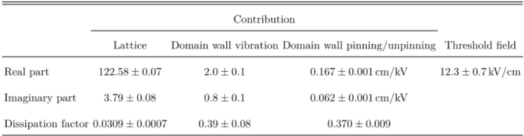
respec-tively to domain wall vibrations and domain wall pinning/unpinning (jump) and depend on the domain wall density. The coefficients are extracted using the Levenberg-Marquat method, which consists of minimizing the quadratic error, and their values are given in the Table.Itogether with the associated uncertainties. The data above 75 kV/cm have not been taken into account for the fit since they deviate from the Rayleigh behavior.
The presence of the Rayleigh behavior in the antiferroelectric material shows the ferro-electric contribution to the permittivity since antiferroferro-electric domain wall movements do not exist under the action of an homogeneous electric field22,30. Only ferroelectric domain wall motions are taken into account by the hyperbolic law which confirms the presence of a ferroelectric phase. However, the value of the Rayleigh parameter α′
r is three orders of
magnitude smaller than the one of PbZr1 – xTixO312,18but almost of the same order as in soft
ferroelectric thin film Ba1 – xSrxTiO321,33. Nevertheless, the parameter α′ris also one order of
7
Table I. Numerical values of the extracted coefficients using the hyperbolic law. The fits are shown into the Fig.3.
Contribution
Lattice Domain wall vibration Domain wall pinning/unpinning Threshold field
Real part 122.58 ± 0.07 2.0 ± 0.1 0.167 ± 0.001 cm/kV 12.3 ± 0.7 kV/cm
Imaginary part 3.79 ± 0.08 0.8 ± 0.1 0.062 ± 0.001 cm/kV
Dissipation factor 0.0309 ± 0.0007 0.39 ± 0.08 0.370 ± 0.009
magnitude higher than for a constrained PZT thin film with almost no domain walls34. The domain wall motions correspond to the center of FORC distribution, inside the triangle with corners (E, Er) =(−250 kV/cm, −250 kV/cm), (250 kV/cm, −250 kV/cm) and (250 kV/cm,
250 kV/cm) where no high hysteron distribution is visible (no global switching polarization). The value representing the domain wall vibration contribution ε′
r −rev is also small
con-firming the low domain wall density and thus a small ferroelectric domain density21. The two parameters ε′
r −revand α′rallow to calculate the threshold field of domain wall pinning
Ethby:20,34,35 Eth= ε′ r −rev α′ r (5) This field represents the degree of wall pinning in the material36 and thus indicates the facility for a domain wall to jump from one pinning center to another. The threshold field for the antiferroelectric thin film is Eth = 12.3 ± 0.7 kV/cm which is higher than what is
observed in the literature34–36indicating deep pinning center for the studied material. This may be due to a small size of the residual ferroelectric clusters which limits the domain wall motions22.
Even if the domain wall density is low, their motion induces high dielectric losses. The dissipation factors of the different contributions to the permittivity, defined as the ratio between the imaginary and the real parts, have been computed and are reported in Table.I. As already seen for other materials, the dissipation factor of the domain wall contributions, vibration and pinning/unpinning, are larger than this of the lattice indicating its dissipative character. The measured dissipation factor for the domain wall pinning/unpinning contri-bution, 0.370 ± 0.009 is slightly smaller than the value predicted by the Rayleigh law (0.42). This is attributed to the low interaction between the ferroelectric domain walls due to a
low domain wall density21,31,33,37and also due to the distribution of the residual ferroelectric clusters in the material22.
In this study, the FORC measurement has been used in order to show a weak ferroelec-tric phase in an antiferroelecferroelec-tric PbZrO3 thin film deposited by sol-gel. This method is
sensitive and complementary to the domain wall motion study by the hyperbolic law. The FORC measurement proves that a low proportion of ferroelectric domains switch at a field corresponding to the E+
AF and E−AF transition fields suggesting that the switching can occur
only when the phase state of the antiferroelectric cells is modified. The measurement of the permittivity as a function of the magnitude of the driving field EACconfirms that there is
no coalescence of ferroelectric domains due to small residual ferroelectric cluster well dis-tributed in the material. This results in a low domain wall density highlighted by the two domain wall motion parameters which are low. Moreover, the domain walls are pinned in deep sites and the unpinning threshold is high. The strength of the FORC measurement applied to antiferroelectric materials, is the ability to obtain the distribution of the coercive fields of the ferroelectric phase, which is not accessible using only the hyperbolic law.
See supplementary material for the P (E) loops measured before and after performing the FORC measurement.
DATA AVAILABILITY
The data that support the findings of this study are available from the corresponding author upon reasonable request.
ACKNOWLEDGMENTS
This work has been performed with the means of the technological platform SMART SENSORS of the French region Pays de la Loire and with the means of the CERTeM (microelectronics technological research and development center) of French region Centre Val de Loire.
9
REFERENCES
1M. H. Park, H. J. Kim, Y. J. Kim, T. Moon, K. D. Kim, and C. S. Hwang,Advanced
Energy Materials 4, 1400610 (2014).
2B. Jaffe,Proceedings of the IRE 49, 1264 (1961).
3X. Hao, J. Zhai, L. B. Kong, and Z. Xu,Progress in Materials Science 63, 1 (2014). 4M. Pešić, M. Hoffmann, C. Richter, T. Mikolajick, and U. Schroeder,Advanced Functional
Materials 26, 7486 (2016).
5K. Karda, A. Jain, C. Mouli, and M. A. Alam,Applied Physics Letters 106, 163501 (2015). 6R. Pike,Phys. Rev. B 68, 1 (2003).
7R. J. Harrison and J. M. Feinberg, Geochemistry, Geophysics, Geosystems 9 (2008),
10.1029/2008GC001987.
8L. Mitoseriu, C. E. Ciomaga, V. Buscaglia, L. Stoleriu, and D. Piazza, Journal of the
European Ceramic Society 27, 3723 (2007).
9I. Fujii, E. Hong, and S. Trolier-Mckinstry, Ultrasonics, Ferroelectrics, and Frequency
Control, IEEE Transactions on 57, 1717 (2010).
10L. Mitoseriu, L. Stoleriu, A. Stancu, C. Galassi, and V. Buscaglia,Processing and
Appli-cation of Ceramics 3, 3 (2009).
11D. Ricinschi, A. Stancu, L. Mitoseriu, P. Postolache, and M. Okuyama, Journal of
Opto-electronics and Advanced Materials 6, 623 (2004).
12W. Zhu, I. Fujii, W. Ren, and S. Trolier-McKinstry, Journal of Applied Physics 109,
064105 (2011).
13L. Stoleriu, A. Stancu, L. Mitoseriu, D. Piazza, and C. Galassi,Phys. Rev. B 74 (2006),
10.1103/physrevb.74.174107.
14M. Hoffmann, T. Schenk, M. Pešić, U. Schroeder, and T. Mikolajick, Applied Physics
Letters 111 (2017), 10.1063/1.5003612.
15A. P. Roberts, Q. Liu, C. J. Rowan, L. Chang, C. Carvallo, J. Torrent, and C.-S. Horng,
Journal of Geophysical Research: Solid Earth 111, n/a (2006).
16A. R. Muxworthy,Journal of Geophysical Research 110 (2005), 10.1029/2004jb003195. 17L. Cima, E. Laboure, and P. Muralt,Review of Scientific Instruments 73, 3546 (2002). 18W. Zhu, I. Fujii, W. Ren, and S. Trolier-McKinstry,Journal of Materials Science 49, 7883
(2014).
19D. V. Taylor and D. Damjanovic,Journal of Applied Physics 82, 1973 (1997).
20C. Borderon, R. Renoud, M. Ragheb, and H. W. Gundel, Applied Physics Letters 98,
112903 (2011).
21K. Nadaud, C. Borderon, R. Renoud, and H. W. Gundel,Journal of Applied Physics 119,
114101 (2016).
22M. D. Coulibaly, C. Borderon, R. Renoud, and H. W. Gundel,Applied Physics Letters
117, 142905 (2020).
23P. Ayyub, S. Chattopadhyay, R. Pinto, and M. S. Multani,Phys. Rev. B 57, R5559 (1998). 24G. Catalan and J. F. Scott,Nature 448, E4 (2007).
25L. Pintilie and M. Alexe,Applied Physics Letters 87, 112903 (2005). 26X. Dai, J.-F. Li, and D. Viehland,Phys. Rev. B 51, 2651 (1995).
27K. Boldyreva, D. Bao, G. L. Rhun, L. Pintilie, M. Alexe, and D. Hesse,Journal of Applied
Physics 102, 044111 (2007).
28L. Pintilie, K. Boldyreva, M. Alexe, and D. Hesse,Journal of Applied Physics 103, 024101
(2008).
29Z. Luo, X. Lou, F. Zhang, Y. Liu, D. Chang, C. Liu, Q. Liu, B. Dkhil, M. Zhang, X. Ren,
and H. He,Applied Physics Letters 104, 142904 (2014).
30K. Vaideeswaran, K. Shapovalov, P. V. Yudin, A. K. Tagantsev, and N. Setter,Applied
Physics Letters 107, 192905 (2015).
31J. E. García, R. Pérez, and A. Albareda,Journal of Physics: Condensed Matter 17, 7143
(2005).
32K. Nadaud, C. Borderon, R. Renoud, A. Ghalem, A. Crunteanu, L. Huitema, F.
Dumas-Bouchiat, P. Marchet, C. Champeaux, and H. W. Gundel,Applied Physics Letters 112, 262901 (2018).
33K. Nadaud, C. Borderon, R. Renoud, and H. W. Gundel,Journal of Applied Physics 117,
084104 (2015).
34C. Borderon, A. E. Brunier, K. Nadaud, R. Renoud, M. Alexe, and H. W. Gundel,Scientific
Reports 7 (2017), 10.1038/s41598-017-03757-y.
35C. Borderon, R. Renoud, M. Ragheb, and H. W. Gundel,Applied Physics Letters 104,
072902 (2014).
36N. B. Gharb and S. Trolier-McKinstry,Journal of Applied Physics 97, 064106 (2005).
11
37J. E. García, R. Pérez, D. A. Ochoa, A. Albareda, M. H. Lente, and J. A. Eiras,Journal
of Applied Physics 103, 054108 (2008).
![[PDF] Formation d’initiation à Microsoft Office Word 2010 | Cours informatique](data:image/gif;base64,R0lGODlhAQABAIAAAP///wAAACH5BAEAAAAALAAAAAABAAEAAAICRAEAOw==)