Publisher’s version / Version de l'éditeur:
Vous avez des questions? Nous pouvons vous aider. Pour communiquer directement avec un auteur, consultez la
première page de la revue dans laquelle son article a été publié afin de trouver ses coordonnées. Si vous n’arrivez
pas à les repérer, communiquez avec nous à [email protected].
Questions? Contact the NRC Publications Archive team at
[email protected]. If you wish to email the authors directly, please see the
first page of the publication for their contact information.
https://publications-cnrc.canada.ca/fra/droits
L’accès à ce site Web et l’utilisation de son contenu sont assujettis aux conditions présentées dans le site
LISEZ CES CONDITIONS ATTENTIVEMENT AVANT D’UTILISER CE SITE WEB.
Ocean Engineering, 220, 15 January 2021, pp. 1-16, 2021-01-12
READ THESE TERMS AND CONDITIONS CAREFULLY BEFORE USING THIS WEBSITE.
https://nrc-publications.canada.ca/eng/copyright
NRC Publications Archive Record / Notice des Archives des publications du CNRC :
https://nrc-publications.canada.ca/eng/view/object/?id=03959f96-ff28-4df6-b4ca-c2d82a0599b6
https://publications-cnrc.canada.ca/fra/voir/objet/?id=03959f96-ff28-4df6-b4ca-c2d82a0599b6
NRC Publications Archive
Archives des publications du CNRC
This publication could be one of several versions: author’s original, accepted manuscript or the publisher’s version. /
La version de cette publication peut être l’une des suivantes : la version prépublication de l’auteur, la version
acceptée du manuscrit ou la version de l’éditeur.
For the publisher’s version, please access the DOI link below./ Pour consulter la version de l’éditeur, utilisez le lien
DOI ci-dessous.
https://doi.org/10.1016/j.oceaneng.2020.108451
Access and use of this website and the material on it are subject to the Terms and Conditions set forth at
CFD based form factor determination method
Korkmaz, Kadir Burak; Werner, Sofia; Sakamoto, Nobuaki; Queutey, Patrick;
Deng, Ganbo; Yuling, Gao; Guoxiang, Dong; Maki, Kevin; Ye, Haixuan;
Akinturk, Ayhan; Sayeed, Tanvir; Hino, Takanori; Zhao, Feng; Tezdogan,
Tahsin; Demirel, Yigit Kemal; Bensow, Rickard
Ocean Engineering 220 (2021) 108451
Available online 12 January 2021
0029-8018/Crown Copyright © 2021 Published by Elsevier Ltd. All rights reserved.
CFD based form factor determination method
Kadir Burak Korkmaz
a,b,*, Sofia Werner
a, Nobuaki Sakamoto
c, Patrick Queutey
d,
Ganbo Deng
d, Gao Yuling
e, Dong Guoxiang
e, Kevin Maki
f, Haixuan Ye
f, Ayhan Akinturk
g,
Tanvir Sayeed
g, Takanori Hino
h, Feng Zhao
i, Tahsin Tezdogan
j, Yigit Kemal Demirel
j,
Rickard Bensow
baSSPA Sweden AB, Chalmers Tv¨argata 10, Box 24001, Se-400 22, G¨oteborg, Sweden bChalmers University of Technology, Sweden
cNational Maritime Research Institute (NMRI), Japan dLHEEA, CNRS Ecole Centrale de Nantes, France
eShanghai Ship and Shipping Research Institute (SSSRI), China fCSHL University of Michigan, USA
gOcean, Coastal and River Engineering (OCRE), NRC, Canada hYokohama National University, Japan
iChina Ship Scientific Research Centre (CSSRC), China jUniversity of Strathclyde, United Kingdom
A R T I C L E I N F O Keywords: Ship resistance Form factor CFD Scale effects
Combined CFD/EFD Methods Experimental uncertainty analysis
A B S T R A C T
The 1978 ITTC Power Prediction method is used to predict the propulsive power of ships through towing tank testing. The form factor approach and its determination in this method have been questioned. This paper in-vestigates the possibility to improve the power predictions by introducing Combined CFD/EFD Method where the experimental determination of form factor is replaced by double body RANS computations applied for open cases KVLCC2 and KCS, including first-time published towing tank tests of KVLCC2 at ballast condition including an experimental uncertainty analysis specifically derived for the form factor. Computations from nine organi-sations and seven CFD codes are compared to the experiments. The form factor predictions for both hulls in design loading condition compared well with the experimental results in general. For the KVLCC2 ballast con-dition, majority of the form factors were under-predicted while staying within the experimental uncertainty. Speed dependency is observed with the application of ITTC57 line but it is reduced with the Katsui line and nearly eliminated by numerical friction lines. Comparison of the full-scale viscous resistance predictions obtained by the extrapolations from model scale and direct full-scale computations show that the Combined CFD/EFD Method show significantly less scatter and may thus be a preferred approach.
1. Introduction
Performance prediction of a ship is one of the most important tasks during the design phase. As a ship design progresses from beginning to end, the required confidence interval for the prediction method in-creases. According to the majority of commercial tendencies presented by shipyards and ship owners, towing tank tests are still considered as the last step of the performance prediction. Additionally, legal author-ities consider towing tank testing as a mandatory step in their evalua-tions such as EEDI calculaevalua-tions as enforced by IMO (2011) where the applicable ships must go through the pre-verification by model testing
during the design phase of a new ship.
Towing tank testing has remained as the only practice for more than a century with high accuracy to predict the performance of a ship in deep and calm water since William Froude introduced the extrapolation procedures in the 1870s. The foundation of the International Towing Tank Committee (ITTC) in 1933, lead to improved and standardized procedures in nearly all aspects of performance prediction. An important step towards a common prediction method was taken in 1973 when computer programs with different assumptions and extrapolation methods were created by SSPA as requested by the ITTC (Lindgren and Dyne, 1980). Ten institutions known to have access to sea trials for
* Corresponding author. SSPA Sweden AB, Sweden.
E-mail address: [email protected] (K.B. Korkmaz).
Contents lists available at ScienceDirect
Ocean Engineering
journal homepage: www.elsevier.com/locate/oceaneng
https://doi.org/10.1016/j.oceaneng.2020.108451
different types of ships evaluated each method by starting from their model test results to calculate the shaft power and propeller rate of revolution (ITTC, 1978). The 1978 ITTC Performance Prediction Method emerged as a result of comparing approximately one thousand sea trials to model test predictions and it is still in effect after going through several revisions.
Even though towing tank testing and extrapolation methods have been debated, discussed and improved over decades, there are inherent and well known shortcomings due to scale effects since model tests are carried out at Froude similarity while Reynolds similarity cannot be fulfilled simultaneously. In order to limit the effects of the shortcomings, towing tank facilities must rely on experience and large databases of both model tests and sea trials. Computational Fluid Dynamics (CFD) has been seen as an alternative to towing tank testing because of CFD’s ability to fulfill both Froude and Reynolds similarities while providing a great deal of detail about the flow. However, the accuracy of CFD on prediction of full scale performance is still under concern. Even though several studies presented by Sun et al. (2020) and Niklas and Pruszko (2019) demonstrated that full-scale simulations can provide similar or better power predictions than towing tank experiments, the results from Reynolds Averaged Navier-Stokes (RANS) solvers in full scale is highly dependent on the computational set-up, e.g., the choice of turbulence model and modelling of hull roughness. The results of Lloyd’s Register workshop on ship scale hydrodynamics (Ponkratov, 2016) also confirmed that differences between the numerical setups can lead to very diverse predictions on both power and propeller turning rate. Un-like the limited full scale verification and validation (V&V) studies mainly due to lack of full scale test data, assessment of state of the art in CFD methods in model scale has been a well established practice since 1980 Larsson et al. (2014). According to the resistance statistics of
Larsson et al. (2014), the mean comparison error in per cent of the measured data value is − 1.7% and − 1.3% for KVLCC2 and KCS in fixed trim and sinkage condition while the standard deviations are 1.3% and 1.2% of the data value, respectively. It was also noted that the mean comparison error and standard deviation in self-propelled cases are considerably higher than those in the resistance cases (Larsson et al., 2014).
As identified by the Combined CFD/EFD Methods ITTC Specialist Committee, combination of EFD and CFD could be a feasible solution to increase the accuracy of power predictions instead of choosing EFD or CFD for the time being. If a part of the model testing or extrapolation procedure causes higher uncertainty than the numerical uncertainty and physical modelling errors of the CFD applications, accuracy will be increased. In the 1978 ITTC Performance Prediction method, the form factor has been identified by the Specialist Committee as one of the major causes of uncertainties, due to the Prohaska method (Prohaska,
1966) and scale effects on form factor for the determination of full scale resistance of ships. Form factor determination method suggested by
Prohaska (1966) was recommended by 14th ITTC meeting (ITTC, 1975) when standardized performance prediction procedures were formulated and debated. During the formulation of the 1978 ITTC Power Prediction method, the form factor concept was found superior to 2-D methods such as the 1957 Power Prediction Method as it led to a better ship-model correlation (ITTC, 1978). The form factor determination method remained as the Prohaska method. However, the main issue with the Prohaska method was described by the ITTC as stated below:
“The problems of ships with partly submerged bulbous bows and the effects of wave breaking resistance for blunt bow forms need further consideration; in both cases it is probably advisable to lower the … speed limits. Future developments for the determination of form factors on a more scientific basis is expected from the Resistance Committee” (ITTC, 1978)
In the 1978 ITTC Power Prediction method, the form factor concept of Hughes (1954) was adopted. It suggests that viscous resistance of a ship can be expressed in relation to a two-dimensional turbulent friction line and the form factor is independent of Reynolds number. As it will be explained in more detail in Section 2, the Prohaska method can be replaced by model scale double body CFD computations which is one of the least numerically complicated CFD applications since modelling of propulsors, free surface and roughness are omitted.
After the form factor determination method, the second error source was identified as the scale effects or speed dependency on form factor. When the 1978 ITTC method was accepted there has been substantial evidence on the scale effects on form factor with ITTC-57 line ITTC (1978). Further re-analysis of geosim test data performed by García G´omez (2000) and Toki (2008) confirmed the scale effects. Additionally, CFD studies performed by Pereira et al. (2017) showed that the speed dependency of form factors with the ITTC-57 line were larger than the numerical uncertainties. Terziev, Tezdogan and Incecik (2019) also showed that form factor is Reynolds number dependent and additionally suggested that the form factor varies with Froude number. The CFD investigations presented by Raven et al., 2008; Wang et al. (2015);
Dogrul et al. (2020) and Korkmaz, Werner and Bensow (2019a) sup-ported the existence of scale effects or speed dependency on form factor and indicated that the main cause of the scale effects are due to the ‘ITTC 57 model-ship correlation line’ rather than the hypothesis of Hughes (1954). CFD based form factor methods were investigated by Korkmaz et al. (2019a) and Wang et al. (2019) in further detail for sensitivity of form factor to grid density and type, speed dependency, presence of rudder, sinkage and trim. The latter investigation also demonstrated that CFD based form factors correlated better with the sea trials compared to the Prohaska method.
As a continuation of the initial study started by the Combined CFD/ EFD Methods Specialist Committee, in this paper CFD based form factor methods have been investigated as an alternative method to the Pro-haska method. KVLCC2 in design and ballast loading condition; KCS in design loading condition are computed at two speeds at both model and full scale. The model tests of KVLCC2 in ballast loading condition per-formed at SSPA’s towing tank and the resistance data together with the measurement uncertainty analysis is presented for the first time in the literature. Wide range of CFD methods and setups are compared with the contribution from 9 different organisations and 7 different CFD codes. In order to quantify the sensitivity of different CFD approaches on form factor, non-ideal CFD setups are also computed and discussed. The scale effects on the form factor are presented by using the friction line pro-posed by Katsui et al. (2005) and numerical friction lines suggested by
Korkmaz et al., 2019b in comparison to form factor based on the ITTC 57 model-ship correlation line.
The following research questions are aimed to be answered by this study.
•Can CFD based form factors with state-of-the-art CFD codes be an alternative or supplement to the Prohaska method?
•Which CFD methods and setups are not fit for reliable CFD based form factor predictions?
•Can the scale effects on form factor be prevented?
•Should the full scale simulations replace the extrapolation methods for full scale resistance predictions?
This paper is structured as follows: Section 2 describes the back-ground of the form factor concept and its determination by experimental methods. The flow solvers, numerical methods, computational domain and boundary conditions, procedure of CFD based form factor calcula-tion are presented in Seccalcula-tion 3. The computational conditions and de-tails of the KVLCC2 towing tank tests in ballast condition are presented
in Section 4. In Section 5, results and discussions are presented and conclusions are summarized in Section 6.
2. Background of the form factor concept and experimental determination methods
The form factor concept has been long discussed since the early 20th century. ITTC (1957) stated that ship resistance extrapolation based on three dimensional analysis (such as form factor approach) has been considered when the ITTC 1957 line was selected. In fact, some re-searchers believed that a two dimensional flow line is not sufficient for the extrapolation problem ITTC (1957), but rather that each hull form requires a separate extrapolator such as Hughes (1954).
The definition of form factor as described by Hughes was adopted by the ITTC (1972) and it is still in practice. The wave-making resistance depends on the Froude number and at low speeds it becomes negligible for most hulls. Thus in carefully conducted experiments where care is taken with regard to turbulence stimulation, measurement accuracy at low speeds and good surface finish, a point in the CT curve can be found.
From this point towards smaller Froude numbers, the curve of CT is
‘sensibly’ parallel to the two dimensional turbulent friction line. This is called by Hughes the ‘low Froude number run-in’ point (Hughes, 1954). The total resistance curve is formulated as,
CT = CF + Cform + CW,
Cform = k CF, (1)
where CF is the resistance equivalent to a flat plate in two dimensional
flow, Cform is form resistance due to the shape of the hull, CW is wave
resistance and k is the form factor. Cform is proportional to CF when the
flow is turbulent and the given hull is smooth, streamlined (without separation) and in symmetrical form when towed in zero incidence angle. Cform is made up of components due to additional skin friction caused by curvature effects, flow in transverse directions and eddy- making (Hughes, 1954).
As Hughes (1954) described, form factor for a hull can be determined by the ratio CT/CF at the “run-in point” since the CW is small enough be
Fig. 2. Example of Prohaska plot in design ballast condition. Table 1
Participants and methods.
Organisation Acronym Code ID Turbulence model Wall model Discretization Grid Type Type Order
CSHL University of Michigan UM OpenFOAM 1 Spalart-Allmaras, k − ω SST WF FV 2 U China Ship Scientific Research Center CSSRC NaViiX 2 RNG k − ε WF FV 2 S Ecole Centrale de Nantes ECN/CNRS ISIS-CFD 3 EASM, k − ω SST WF, WR FV 2 U National Maritime Research Institute NMRI NAGISA 4 EASM, k − ω SST WF, WR FV 3 OS Ocean, Coastal and River Engineering NRC-OCRE OpenFOAM 5 k − ω SST WF FV 2 U SSPA/Chalmers University of Technology SSPA/CTU SHIPFLOW 6 EASM, k − ω SST WR FV 2 OS
Shanghai Ship and Shipping Research Institute SSSRI Star-CCM+ 7 k − ω SST, RSTM, Realizable k − ε WF FV 2 U
Strathclyde University Strathclyde Star-CCM+ 8 k − ω SST WF FV 2 U Yokohama National University YNU SURF 9 EASM, k − ω SST WR FV 2 S
FV Finite Volume; WR wall resolved; OS Overlapping Structured; S Single Block Structured; U Unstructured; WF wall functions.
Table 2
Computational conditions.
Computational conditions LPP (m) Scale factor Draught at FP(m) Draught at AP(m) S/L2 Vm (m/s) Vs (kn) Rem Res Fn
KVLCC2 (design) 320 58 20.8 20.8 0.2682 0.878 13 4.11 × 10⁶ 1.80 × 10⁹ 0.119 1.047 15.5 4.90 × 10⁶ 2.14 × 10⁹ 0.142 KVLCC2 (ballast) 320 45.714 8.6 11.4 0.1921 0.989 13 6.24 × 10⁶ 1.80 × 10⁹ 0.119 1.179 15.5 7.44 × 10⁶ 2.14 × 10⁹ 0.142 KCS (design) 230 31.6 10.8 10.8 0.1803 1.281 14 7.33 × 10⁶ 1.39 × 10⁹ 0.152 2.196 24 1.26 × 10⁷ 2.39 × 10⁹ 0.260
neglected in Eq. (1). However, in order to find the run-in point, the speed range for the resistance test must be extended to very low Fn and Re numbers which is rather challenging as the Re at such low speeds might be too low for turbulence stimulators to make sure the flow around the hull is turbulent. Additionally, certain scatter in resistance measure-ments at low speeds due to worsening measurement accuracy for small forces can hinder the form factor determination, as Lindgren and Dyne (1980) indicated.
As an alternative, Prohaska (1966) suggested a simple method to derive the form factor from resistance tests. When no separation is present, the form factor is expressed as
CT =CW + (1 + k)CF. (2)
The wave resistance coefficient, CW, can be expressed as Eq. (3)
which is the asymptotic expansion formula of wave-making resistance coefficient presented by Inui as cited in Toki (2008),
CW =a × Fr4 + b × Fr8 + c × Fr12 + d × Fr16. (3)
CT at model scale is then expressed together with the Inui’s
asymp-totic expansion formula, Eq (3), as
CTm= (1 + k) × CF +CW = (1 + k) × CF +a × Fr4 +b × Fr8
+ c × Fr12 +d × Fr16. (4)
Neglecting the higher order terms of Eq. (4) as they are close to zero at low Froude numbers and dividing each sides by CF, the following
linear relationship is obtained,
CTm
/
CF≈ (1 + k) + a × Fr4
/
CF. (5)
Prohaska (1966) noted that when results of approximately 200 model tests have been plotted with Eq. (5), for Fn between 0.1 and 0.2, the CT/CF values for a great majority of the models plot on straight lines.
One of the exceptions when the CT/CF values deviated from the straight
line and points correlate with concave curves is with hull forms with
CB>0.75. It was suspected that 1 + k may be speed dependent, or as
Prohaska (1966) stated “can be easily explained by as resulting from increasing trim on the bow.” The other hull form Prohaska observed
where CT/CF values plot on convex curves was twin-screw models with
appendages and for some models with full aft body lines, which was explained by a certain separation (Prohaska, 1966). It should be noted that detection of flow separation and treatment of deeply submerged transoms remain as challenges of the Prohaska method. However, the main weakness of the Prohaska method discussed in modern literature is the bulbous bow near the water surface and partly submerged bulbous bow in partial loaded conditions which is not mentioned by Prohaska (1966) since the model test data used by Prohaska dates back to 1966 and earlier when bulbous bows were not a popular design concept.
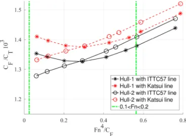
In order to illustrate this aspect of the uncertainty of form factor determination caused by the Prohaska method, the model test results of the resistance curves of two hulls are plotted as in Eq. (5) and presented in Fig. 1 and Fig. 2. In order to protect the confidentiality of the test results, CT/CF curves shown in Figs. 1 and 2 are slightly tilted without
changing neither the general shape of the curves nor the relative posi-tion of each measurement point at the same Froude number. Hull-1 and Hull-2 are only different in bulbous bow and they are geometrically similar for the rest of the hull (95% identical hulls). The bulbous bow of Hull-1 features a mild goose-neck design (distinctly convex upper stem profile of the bulb) and has significantly more volume close to water surface at design loading condition compared to Hull-2. As can be seen from Fig. 1, not all CT/CF values of Hull-1 in design loading condition
follow a straight line within the recommended Fn range, which is be-tween 0.1 and 0.2 as indicated by the green vertical lines. The concave shape of CT/CF values for Hull-1 can be explained by the presence of
significant and often steep waves that are generated by the bulb. The waves generated at significantly lower Froude numbers than the design speed are too short in wave length to favourably interact with the bow waves of the hull. On the other hand, CT/CF values of Hull-2 reasonably
follow a straight line which suits the description of Prohaska (1966)
since the waves are much smaller at low Fn as a result of reduced the pressure gradient and moving the bulb volume away from the water surface. Considering that the two hulls are 95% identical, large differ-ences are observed in CT/CF curves.
The uncertainly with the Prohaska method further increases in the ballast loading conditions as shown in Fig. 2. The CT/CF values of Hull-1
within the recommended range shows a large hump which cannot be used for a line fit. In other words, the wave making resistance cannot be described by Eq. (4) and the linear relationship proposed by Prohaska in Eq. (5) is not valid. In ballast condition at the low speeds, Hull-2 also shows a hump in CT/CF values which was not existent in the design
condition. In order to demonstrate that a different friction line would not have helped, the CT/CF values are also calculated with the Katsui friction
line (Katsui et al., 2005) instead of the 1957 ITTC model-ship correlation line. As seen in Fig. 1, the convex shape of the CT/CF values persists. As
shown in this example, quantifying the uncertainty or error of Prohaska form factor determination method is difficult since it is very sensitive to the hull design. Considering that the bulbous bows are now a common feature of modern ship design, it is hard to advocate the validity and practicality of the Prohaska method for all hull designs and loading conditions.
One further aspect of uncertainty of form factor determination with the Prohaska method originates from the experimental uncertainty, UD.
The uncertainty on form factor can be significantly higher than the experimental uncertainty since it is not directly measured but obtained as a result of data reduction, i.e. regression analysis. This will be dis-cussed thoroughly in Section 4 when the towing tank tests for KVLCC2 in ballast loading condition are presented.
3. Participants and methods
In total 9 different organisations with 7 different CFD codes contributed to the current study. The organisations are listed in Table 1
together with the main features of their methods. The results will be discussed and presented with the ID numbers of the organisations in the
Table 3
Combination of uncertainty in measurement for resistance at Fn = 0.119 and.Fn = 0.142.
Uncertainty Components Uncertainty at 16.0 ◦C
Fn = 0.119 Fn = 0.142
Wetted area 0.080% 0.080%
Speed 0.067% 0.057%
Water temp. 0.002% 0.002% Dynamometer 0.705% 0.492% Repeat test, Deviation 0.470% 0.344% Combined for single test 0.854% 0.609% Repeat test, Deviation of mean 0.210% 0.154% Combined for repeat mean 0.743% 0.525% Expanded for repeat mean 1.487% 1.050%
Table 4
Total resistance coefficient, CT, combined mean measurement uncertainty, UD, number of repeat tests, N, at.16.0∘C.
Fn CT×103 UD N 0.110 3.981 0.84% 4 0.119 3.968 0.74% 5 0.133 3.976 0.60% 4 0.142 4.001 0.52% 5 0.147 4.016 0.51% 4
paper.
Two-equation turbulence models k − ω SST, RNG k − ε, Realizable
k − ε are used by the majority of the computations. Anisotropic models, EASM and RSTM, are not used by all organisations but EASM model is still covering a large portion of the calculations. Only one organisation used the one-equation Spalart-Allmaras model.
Simulations were performed using finite volume codes with 2nd order accurate schemes except one code with 3rd order accurate scheme. The grids used were single or multi-block structured grids (butt-joined, curvilinear or overlapping techniques) and unstructured ones.
Computational domain shape and size varies with each code. Ma-jority of the upstream boundaries are located between 1LPP and 1.5LPP
from the fore perpendicular (FP), but ECN/CNRS and SSPA/CTU are differing from others by using the distance of 5LPP and 0.5LPP,
respec-tively. The downstream extent of the domains varied between 8LPP and
0.8LPP from the aft perpendicular (AP) while the common distance of
downstream extent is between 2LPP and 3LPP. Lateral (both sidewards
and downwards) extend is commonly located between 1.5LPP and 2.5LPP
away from the ship center-plane and free surface plane but two notable exceptions are 1LPP and 4LPP from UM and ECN/CNRS, respectively.
All computations were performed as double model with a symmetry boundary condition at the ship center-plane and free surface plane. Most popular upstream boundary condition is uniform in all variables with the exception of one participant with prescribed pressure. The down-stream conditions are usually zero gradient in the down-streamwise direction except the pressure quantity that is specified. The lateral boundaries are dominated by far field boundary conditions but slip and zero gradient
boundaries are also used. Majority of the computations (approximately 60%) are performed with wall resolved condition and the remaining simulations were performed with wall functions.
The CFD based form factor method considered for this study follows the assumptions of Hughes (1954) and is derived using the relation, (1 + k) = CF +CPV
CF0
= CV
CF0
, (6)
where the frictional resistance coefficient (CF) and viscous pressure
coefficient (CPV) are obtained by the double body CFD simulation. CF0 in
the denominator of Eq. (6) is the equivalent flat plate resistance in two dimensional flow obtained from the same Reynolds number as the computations. In this study, three friction lines are considered: the ITTC- 57 model-ship correlation line (ITTC, 1957), the Katsui line (Katsui et al., 2005) and numerical friction lines proposed by Korkmaz et al. (2019b). It is worth mentioning that the ITTC-57 line is not a pure friction line but it contains a component of form resistance (11.94% of the friction line of Hughes (1954)). It is included in the scope of the study because it is still the model to ship correlation line recommended by ITTC (2014a).
The shortcomings of the Prohaska method for the hulls with a pro-nounced bulbous bow have been mentioned in Section 2. In a case when there is just a small gap between the top of the bulb and the still-water surface, a flow separation may be generated around the top of the bulb for the double body simulations. Such flow separation would not occur in free-surface flow; therefore, the form factor obtained from the double
Fig. 3. KVLCC2 in ballast loading condition at.Fn = 0.142
Fig. 4. Prohaska plot of KVLCC2 in ballast loading condition.
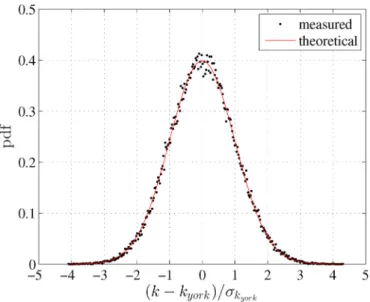
Fig. 5. Probability density function of the form factor of KVLCC2 in ballast
body computation will be affected. Raven et al. (2008) suggested that if the bulb is submerged more by trimming the hull bow down, this issue can be prevented. Another drawback that is shared between CFD and EFD based form factor determination methods is the large submerged transom which may cause flow separation in the wake. The test cases used in this study do not possess the hull form features that may cause aforementioned issues for the CFD based form factor method. Therefore, no corrections have been applied to the double-body flow computations.
4. Test cases and computational conditions
The two hulls used for the current study are: •KVLCC2 with rudder
•KCS with rudder
The KVLCC2 and KCS hulls are designed at the Korea Research Institute for Ships and Ocean Engineering (KRISO) to be used as open test cases for CFD predictions. Extensive towing tank tests and CFD in-vestigations were carried out in the last two decades. Therefore, hull lines and detailed hydrostatics are not presented. The hull and rudder geometries are obtained from Tokyo (2015) and SIMMAN (2008)
workshops for KCS and KVLCC2, respectively.
The computational conditions for the study is presented in Table 2. Non-dimensional quantities, Re and Fn, are based on LPP. The force
co-efficients are non-dimensionalized with the corresponding wetted sur-face coefficients, S/L2PP, to the loading conditions. For each hull and
loading condition, two different speeds were used for the computations in order to investigate the importance and the effect of selecting a speed for the form factor determination. The first speed is chosen in the low side of the regular model testing speed range where CT/CF is close to the
form factor (see Fig. 1) determined by the Prohaska method. The second speed is the design speed of each vessel. Data for resistance tests of KVLCC2 and KCS at design draught are adopted from Van et al. (2011). The resistance test data of the KVLCC2 in ballast loading condition has never been published. Therefore, SSPA determined a typical ballast loading condition for Very Large Crude Carriers (VLCC). Towing tank tests were performed at SSPA’s towing tank including an uncertainty analysis of the resistance tests.
4.1. Uncertainty analysis of KVLCC2 resistance tests in ballast draught
A KVLCC2 model with a scale factor of 45.714, made of the plastic foam material Divinycell, was manufactured with 5-axis CNC milling machine at SSPA. After the surface finishing and painting, the model was scanned with a 3D scanner to check the tolerances described in ITTC (2014c). A trip wire is mounted at 5% of LPP aft from the fore
perpen-dicular for the turbulence stimulation. The hull model is equipped with a dummy propeller hub and a rudder. The geometry of the rudder is ob-tained from SIMMAN (2008) and the dummy hub is a simple cylinder with the diameter of the boss end of the hull.
The model tests were performed in SSPA’s towing tank which is 260 m long, 10 m wide and 5 m deep. The model tests were carried out in mid-May 2020. The total resistance, sinkage and trim were measured at Froude numbers varying between 0.110 and 0.147. The mid-sectional area of the KVLCC2 model in ballast loading condition is 0.155% of the towing tank section area. Therefore, no blockage correction is applied. The tests were started by performing one run per Fn = 0.119 and Fn = 0.142 speeds, respectively. It was followed by starting from the lowest Fn and the speed is increased successively at each run after 20 min of waiting time. There was a total of five repeat tests for Fn = 0.119 and Fn = 0.142, while the rest of the speeds were repeated four times. The uncertainty regarding the wetted surface area are quantified by measuring the model ballasting. The model and weights (calibrated 25 separate pieces) used for ballasting the model were weighted by two digital scales (ITTC, 2014b). Resulting uncertainties on the wetted
surface are presented in Table 3 for Fn = 0.119 and Fn = 0.142 speeds. The relative uncertainty of the towing speed is assessed by the bias limit of the towing carriage and they are presented in Table 3.
The water temperature during the tests showed less than 0.1∘C
variation. As described in ITTC (2014b), the measured resistance is converted to 16.0∘C which was used for the CFD computations prior to
the tests. The corresponding component of uncertainties in resistance due to temperature variation are presented in Table 3. The model was scanned and checked at the model workshop. The thermal deformation of the model is expected to be limited as the temperature difference between the model workshop and the towing tank is less than 5∘C.
An in-house design dynamometer with a sampling rate of 10 Hz was used for measuring the resistance. The measurement at each speed is obtained by averaging the time history of the signal as described in ITTC (2014b). The standard uncertainty of average of the sampling history varied between 0.0008% and 0.0015%, while the average of all repeti-tions is 0.0011%. Therefore, the uncertainty of one reading from the Data Acquisition System (DAS) is negligible. The dynamometer avail-able at the time of the towing tank tests were calibrated to a much greater range than the maximum model resistance. As a result, the un-certainty regarding to the dynamometer is the dominant source as can be seen in Table 3. The dynamometer calibration was checked after the tests. Additionally, a calibration with a range that was approximately 3 times the maximum model resistance was performed. The uncertainty due to the dynamometer dropped nearly three times with the smaller range which would have halved the total uncertainty in Table 3.
Based on the analysis described in ITTC (2014b), the significant components of uncertainties are combined through RSS (Root-Sum-S-quare). As seen in Table 3, major sources of the uncertainties are orig-inating from the dynamometer (with the large calibration range) and the precision of measurement in the repeat tests. The uncertainty of resis-tance measurements for Fn = 0.119 and Fn = 0.142 are 0.74% and 0.53%, respectively. The expanded uncertainties in Table 3 correspond to the confidence level of 95%.
In Table 4, combined measurement uncertainties are presented in per cent of the measured data value which is the mean total resistance of all repeat tests at each speed. The uncertainties are between 0.51% and 0.84%. As seen in Table 4, it is decreasing with increasing speed because at the high speeds the contribution from the dynamometer decreases.
As mentioned before, one aspect of uncertainty of form factor determination with Prohaska method originates from the experimental uncertainty, UD. In order to illustrate that the uncertainty on form factor
is significantly higher than the experimental uncertainty, the Prohaska plot is presented in Fig. 4 with the error bars representing the experi-mental uncertainties presented in Table 4. Unlike the main discussion point in Section 2, the CT/CF values can be sensibly aligned to a line as
the waves generated at the ballast loading condition were not too sub-stantial as can be seen in Fig. 3.
The regression line in Fig. 4 is obtained by applying the method explained by York et al. (2004). This method considers the experimental uncertainties in the regression progress and predicts the uncertainties in the form factor as well. The resulting regression line is indicated as the York’s method in Fig. 4 where the uncertainty on the form factor is illustrated with an error bar at Fn4/CF=0. The uncertainty of form
factor is calculated as 0.011.
Additionally a Monte Carlo simulation is performed to illustrate the variation on form factor due to measurement uncertainty. For each iteration, all measured point are varied as
C′T= CT +USD × R (7)
where CT is measured point presented in Table 4, USD is the
measure-ment uncertainty and R is normally distributed random number. In every iteration, a new regression line and form factor are calculated with the York et al. (2004) method. The error, k − kyork, obtained from the Monte Carlo simulation is normalized by the uncertainty obtained from
the York et al. (2004) method (σyork) and the probability density function (pdf) is calculated. As can be seen in Fig. 5, the Monte Carlo simulation indicates a normal distribution for the normalized error of the form factor and the standard deviation of the error is equal to the uncertainty obtained from the York et al. (2004) method. As a result of using both methods, the uncertainty of the form factor is calculated as 0.022 cor-responding to 1.9% of 1 + k for the 95% confidence interval.
5. Results
The analysis of approximately 300 double body simulations of the two hulls under the conditions stated in Table 2 is discussed in this section.
5.1. Friction and viscous pressure resistance in model scale
Firstly, friction and viscous pressure resistance coefficients are investigated since only these quantities are directly computed by CFD codes. Instead, form factor is a combination of the two computed values and a friction line. Therefore, detecting the tendencies between different CFD methods might be hindered due to errors cancelling each other.
5.1.1. Uncertainty analysis
Uncertainty analysis is performed to quantify the grid uncertainty (UG) by SHIPFLOW and NAGISA codes. For the grid dependence study,
five geometrically similar grids were used with the former code and systematically refined grid triplets are prepared for latter. Both SHIP-FLOW and NAGISA performs the simulations in double precision in order to eliminate the round-off errors. The iterative uncertainties were quantified by the standard deviation of the force in percent of the average force over the last 10% of the iterations. Iterative uncertainty for CF and CPV were kept below 0.01% and 0.15% for SHIPFLOW, while
iterative uncertainty for CF, CPV and CT for NAGISA were kept below
0.1% of their mean values for all simulations in model scale. Therefore, it was assumed that the numerical errors are dominated by the dis-cretization errors and both iterative errors and round-off errors are neglected.
For SHIPFLOW, the procedure proposed by Eça and Hoekstra, 2014
was used to predict the grid uncertainties which are presented for the finest grid as a ratio of the computed value (UG%S1) in Table 5. In order
to quantify the grid uncertainty for NAGISA, three criteria are adopted, e.g. Factor of Safety (FS) method proposed by Xing and Stern (2009), Correction Factor (CF) method and Grid Convergence Index (GCI) method shown in ITTC (2017). Table 6 summarizes the results for KVLCC2 in design and ballast loading condition and KCS. In the cases where monotonic convergence is not obtained, the solution change is less than 1% of S1 (ε21ε32). Therefore, UG is omitted and noted with a " - "
symbol in Table 6.
5.1.2. Statistics of CF and CPV
The simulations in model scale comprise computations from seven different codes and six different turbulence models with wall functions and wall resolved approaches. These computations include not only the CFD setups according to the best practice guidelines (BPG) or standard settings but also setups that deviated from recommended guidelines since one of the aim of this study is to identify the methods that are not well suited for the form factor determination. In order to differentiate the contribution of the computations with deliberately made undesired settings, two different populations are considered when the statistics, such as mean and standard deviation, are calculated. The first popula-tion (denoted as P1) includes all simulapopula-tions and the second populapopula-tion (denoted as P2) is the computations performed with best practices or standard settings of each code. It was deemed necessary to add one more population as a sub-population of the latter because of concerns on the statistics being biased by a code significantly outnumbering others in some test cases. Therefore, the third population (denoted as P3) is ob-tained by selecting the computations from the two finest grids of each code per CFD approach such as turbulence model, wall treatment. This selection is based on the number of cells under the assumption that fine grids have less discretization uncertainty.
The mean and standard deviation of CF and CPV for each condition is
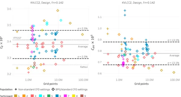
calculated with the three previously mentioned populations. As pre-sented in Table 7 and Table 8, it is observed that statistics of different populations of the same condition showed limited variation except KVLCC2 in design condition which is the condition many of the delib-erate variations were applied to CFD setups. In Fig. 6, the Population 2 and simulations with non-desired CFD set-ups are visualised by dividing all the computations for KVLCC2 in design condition into two groups: computations with non-standard CFD set-ups, and simulations with the best practice guidelines (BPG) or standard CFD set-ups. The small dif-ference in statistics between the Population 2 and 3 shows that the statistics are not biased even though some test cases are overcrowded with simulations from one code. The computations performed with the best practices or the standard settings of each code (Population 2) will be used for the rest of the analysis, except when the results of deliberate variations of CFD setups are discussed.
Friction and viscous pressure resistance coefficients.CF and CPV
Table 5
Estimated grid uncertainties of SHIPFLOW for KVLCC2 and KCS in model scale for EASM and k − ω SST turbulence models, in percentage of the computed result of the finest grid S1.UCT = UCF + UCPV.
UG Turbulence
model Fn KVLCC2 (design) KVLCC2 (ballast) KCS (design) 0.119 Fn 0.142 Fn 0.119 Fn 0.142 Fn 0.152 Fn 0.26 CF EASM 1.0 1.2 1.3 1.2 3.5 3.2 k− ω SST 1.1 1.4 0.9 1.0 5.9 9.6 CPV EASM 1.0 3.0 17.9 5.1 32.5 19.4 k− ω SST 1.1 3.0 23.0 10.8 30.2 21.0 CT EASM 1.0 1.6 3.6 1.8 6.7 5.0 k− ω SST 1.1 1.7 3.7 2.3 8.4 10.7 Table 6
Estimated grid uncertainties (UG) of NAGISA for KVLCC2 and KCS in model scale for EASM turbulence model, in percentage of the computed result of the finest grid S1.
UG Method KVLCC2 (design) KVLCC2 (ballast) KCS (design)
Fn 0.142 Fn 0.119 Fn 0.142 Fn 0.26 CF FS 3.1 2.1 2.0 – CF 3.8 2.4 2.3 – GCI 0.3 1.2 1.2 – CPV FS 0.1 – – 4.7 CF 0.1 – – 5.1 GCI 0.1 – – 3.0 CT FS – 0.3 0.3 – CF – 0.2 0.2 – GCI – 0.2 0.2 – Table 7
The mean and standard deviation of CF for KVLCC2 and KCS in model scale.
Quantity KVLCC2 (design) KVLCC2 (ballast) KCS (design) Fn 0.119 Fn 0.142 Fn 0.119 Fn 0.142 Fn 0.152 Fn 0.26 Mean (P1) 3.462 3.381 3.298 3.21 3.112 2.893 Mean (P2) 3.47 3.394 3.298 3.215 3.105 2.892 Mean (P3) 3.455 3.376 3.298 3.215 3.095 2.885 σ (P1) 2.7% 2.5% 2.5% 2.4% 2.0% 1.6% σ (P2) 2.5% 2.6% 2.5% 2.5% 2.0% 1.6% σ (P3) 2.9% 2.8% 2.5% 2.6% 1.9% 1.8%
in model scale for KVLCC2 in both loading conditions and KCS in design condition are presented versus grid size (in logarithmic scale) in Fig. 7
and Fig. 8. In order to have references for the friction resistance coef-ficient, the ITTC-57 line and the Katsui line are plotted in Fig. 7.
As can be seen in Figs. 7 and 8, there is no distinct dependence of results on the grid size. Note that this is a comparison of unsystemati-cally varied methods and grids. However, other dependencies such as the turbulence modelling and the wall treatment were found both on CF
and CPV. The frictional resistance coefficients from UM (Participant 1)
and SSPA/CTU (Participant 6) indicate a strong dependence on
turbulence model while this effect is rather limited on the results of ECN/CNRS (Participant 3), NMRI (Participant 4) and YNU (Participant 9). The viscous pressure coefficients from ECN/CNRS and SSPA/CTU show larger dependence on turbulence models than the others. ECN/ CNRS and NMRI performed simulations both with wall resolved and wall function. Both codes indicate a significant dependence on wall treatment especially for CF but also for CPV which is less sensitive to the
wall treatment than the frictional resistance component.
Variations of CFD setups. The previously mentioned CFD setups
that varied from recommended guidelines on KVLCC2 in design condi-tion have been applied by UM, ECN/CNRS, SSPA/CTU and SSSRI. UM (Participant 1) varied grids focusing specifically to the grid resolution near the wall using two turbulent models. As can be seen in Fig. 9, where all computations on KVLCC2 in design condition are presented, k − ω SST and Spalart-Allmaras turbulence models shows high sensitivity on CF to both grid refinement and y+variation. However, the variation on
CPV is limited except for the coarsest grid set.
ECN/CNRS (Participant 3) performed grid variations also with adaptive grid refinement. When wall functions were used, CF and CPV
showed small variation even for the very coarse grids. However, wall resolved simulations of ECN/CNRS are more grid dependent compared
Table 8
The mean and standard deviation of CPV for KVLCC2 and KCS in model scale.
Quantity KVLCC2 (design) KVLCC2 (ballast) KCS (design) Fn 0.119 Fn 0.142 Fn 0.119 Fn 0.142 Fn 0.152 Fn 0.26 Mean (P1) 0.793 0.777 0.504 0.494 0.387 0.33 Mean (P2) 0.789 0.739 0.501 0.49 0.387 0.326 Mean (P3) 0.794 0.745 0.499 0.488 0.393 0.335 σ (P1) 9.2% 13.1% 6.6% 6.2% 7.6% 13.6% σ (P2) 9.7% 9.8% 7.3% 6.9% 9.0% 14.4% σ (P3) 10.2% 10.3% 7.9% 7.5% 9.2% 15.0%
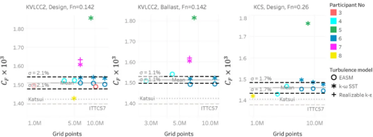
Fig. 6. Frictional coefficient (left) and viscous pressure coefficient (right) in model scale for KVLCC2 hull in design loading condition at Fn. = 0.142
Fig. 7. Frictional coefficient, CF, in model scale for KVLCC2 hull in design loading condition at Fn= 0.142 (left), KVLCC2 in ballast loading condition Fn= 0.142 (center) and KCS hull in design loading condition at Fn= 0.26 (right).
to wall functions. This is explained by the increasing grid resolution near the wall rather than the increase in grid size for the wall resolved computations.
In addition to the systematic grid variations for the grid dependence studies, SSPA/CTU (Participant 6) performed grid variations by coars-ening the grid of the bow and the stern region of the KVLCC2 hull in the longitudinal direction while keeping the rest of the grid the same. For this exercise, the second finest grid and the coarsest grid of the grid dependence study was selected as a starting point. Coarsening the bow and stern regions up to grid density of one third of the starting grids did not show a significant variation on CF but some variation in CPV for the
same turbulence model except for one case. When the coarsest grid was further coarsened in the aft, the CPV was calculated extremely high as
seen in Fig. 6 (highest two values from Participant 6) while the variation of CF was limited. The grid variations of SSPA/CTU on KVLCC2 showed
that when the grid resolution normal to the wall is kept similar, CF and
CPV are more sensitive to the grid density in aftbody than forebody.
Simulations of SSSRI (Participant 7) was performed with three different turbulence models. As can be seen from Fig. 9, both CF and CPV
obtained from Reynolds Stress Turbulence Model (RSTM) were signifi-cantly higher than the realizable k − ε and k − ω SST models with similar grids and average y+values. Additionally, different types of wall
functions were used with realizable k − ε and k − ω SST models while keeping the grids similar. CF and CPV showed only marginal change due
to different wall function type for the k − ω SST model. However, the realizable k − ε model showed a substantial variation in both CF and CPV
due to different wall function treatment. Finally, y+is varied with the
realizable k − ε model. It is observed that when the average y+increases
(from 71 to 112 in steps of 11), CF also increases up to 2% while CPV
decreases up to 4.5% as shown in Fig. 9. Therefore, a significant dependence of y+and wall function treatment on viscous resistance is
observed with the realizable k − ε model.
5.2. CFD based form factors with the ITTC-57 line
CFD based form factors are calculated using Eq. (6) and presented versus the number of grid points in Fig. 10. Note that only the simula-tions performed according to the best practice guidelines or standard settings of each code are presented and logarithmic scale is used in the grid points axis for better clarity. In addition to standard deviation in percentage of (1 +k) and mean of the CFD based form factors (k), form factors determined by model tests of Van et al. (2011) for KVLCC2 and KCS in design condition and KVLCC2 in ballast loading condition of SSPA are plotted in Fig. 10.
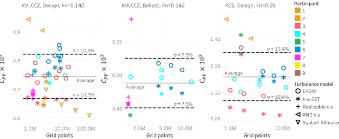
Fig. 8. Viscous pressure coefficient, CPV, in model scale for KVLCC2 hull in design loading condition at Fn= 0.142 (left), KVLCC2 in ballast loading condition Fn= 0.142 (center) and KCS hull in design loading condition at Fn= 0.26 (right).
Fig. 9. CF (left) and CPV (right) in model scale for KVLCC2 hull in design loading condition at Fn= 0.142 against mean y+. y+<1: wall resolved, y+>1: wall function.
Mean of the form factor predictions for the KVLCC2 in design con-dition at Fn = 0.119 and Fn = 0.142 are both close to the form factor determined experimentally. The standard deviation of the form factors obtained from the unsystematically varied methods and grids at both speeds is around 1.9%. If the form factor is used in extrapolation of the model resistance value for this KVLCC2 case, this would cause approx-imately 3% spread in the predicted full-scale resistance (roughness, correlation allowance and air resistance excluded). Number of grid cells among the computations varied between one million to 62 million, However, form factor predictions do not indicate dependence on the number of grid cells.
Mean of the form factor predictions for the KCS in design condition at
Fn = 0.26 is very close to the experimental value. However, at Fn =
0.152, the mean value of form factor is 0.015 smaller than the mean form factor at Fn = 0.26 as shown in Table 9 in Section 5.3. This dif-ference was not as large for the KVLCC2 because the Re difdif-ference be-tween the speeds were small (19%). However, Re difference bebe-tween the speeds for the KCS hull is 71% which is big enough to reveal the speed dependency of the form factor as it is discussed in further detail in Section 5.3. The standard deviation of 1.5% translates to approximately 1% in full scale resistance excluding the contribution of roughness, correlation allowance and air resistance. Note that this is a remarkable result even though such a wide range methods and grids were used since KCS like hulls are the ones that suffers the most from the Prohaska method because of the prominent bulb designs.
All the computations for KVLCC2 in ballast case had to be performed prior to the model tests. The slight discrepancy in water temperature between computations and tests were corrected using ITTC (2014b)
procedures for form factor determination. Form factor predictions for the KVLCC2 in ballast loading condition showed a similar standard de-viation to the other cases. However, the mean value of the form factor is not as close to the experimentally determined form factor as the other cases. As explained in Section 4, uncertainty analysis was performed for the form factor. When the uncertainty of the Prohaska method on the experimentally determined form factor is considered, majority of the
simulations are still within the uncertainty range.
It is observed in Fig. 10 that some form factor predictions are rela-tively far from the experimentally derived form factor. However, it is encouraging to observe that there are some consistent patterns for most of the codes. The form factor was under-predicted similarly by YNU (Participant 9) and ECN/CNRS (Participant 3) for both KVLCC2 and KCS hulls in design condition. Results of SSSRI (Participant 7) are also under- predictions for all the cases. It should be noted that as long as one code with a certain set-up consistently predicts the form factor with the same tendency, application of correlation factors (CP or CA) in the 1978 ITTC Power Prediction method will help to reduce the discrepancies.
CFD Code Dependency. The dependencies and tendencies of each
code for the form factor predictions are plotted in Fig. 11 and Fig. 12. Computations from each code are stacked in separate columns where box-and-whisker plots are placed with markers. The box plot can be identified with the gray color and sized with the lower and upper quartiles. Lines extending from the boxes (whiskers) extend to the data within 1.5 times the interquartile range (IQR). The markers are colored with the turbulence models, shaped according to the wall treatment type and sized according to the number of cells.
Turbulence Model Dependency. The choice of turbulence model
stands out as a decisive element of the CFD based form factors when the results of UM, ECN/CNRS, NMRI and SSPA/CTU are considered. Even if the same code and similar CFD set-ups are used, a significant depen-dence on turbulence models are observed. However, a general trend for each turbulence model cannot be maintained either. For example, ECN/ CNRS (Participant 3), NMRI (Participant 4) and YNU (Participant 9) predicted higher form factors with EASM turbulence model than with
k − ω SST, while this is the opposite with SSPA/CTU (Participant 6). It should be also noted that the form factor predictions from the same turbulence model with different CFD codes are largely scattered. Therefore, the dependence of form factors to the CFD codes surpasses the choice of the turbulence model.
Wall Treatment Dependency. The type of wall treatment and y+
can be considered as significant dependencies of form factor as it was the
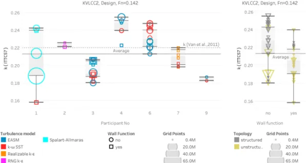
Fig. 10. Form factor, k, based on ITTC-57 line versus grid size for KVLCC2 hull in design loading condition at Fn = 0.142 (top left) and Fn = 0.119 (top right), KCS
case for CF and CPV investigated earlier. ECN/CNRS and NMRI
per-formed computations with the same turbulence models of k− ω SST and EASM and also both participants had simulations with and without wall functions. As can be seen from Figs. 11 and 12, form factor dependence on the wall treatment is observed with both ECN/CNRS (Participant 3) and NMRI (Participant 4), while a significant dependence on y+was
observed with the realizable k − ε model for SSSRI.
On the right side of Figs. 11 and 12, simulations from all codes are sorted with the type of wall treatment. The markers are colored with the type of the grid. The box plots of both KVLCC2 and KCS indicate that interquartile range (IQR) of simulations with wall functions are smaller than wall resolved. However, the distance between the whiskers are similar for both approaches. Although the CFD results as a whole are a product of unsystematically varied methods and grids, the comparison of median values of different wall modelling indicates that simulations with wall functions predict considerably smaller form factors compared to wall resolved approach.
5.3. Form factors with alternative friction lines
As mentioned earlier in Section 1, speed dependency or scale effects have been found on the form factor by the previous investigations. However, it should be noted that the form factors should always be
considered with the friction line used as the physical meaning of speed dependency or scale effects on the form factor is that the viscous resis-tance of a ship is not proportional to the selected friction line. Even if the concept of Hughes (1954) (see Section 2) is true, different sizes of geo-sim models and double body geo-simulations at different Reynolds numbers will result in different form factors as a result of using an ‘improper’ friction line. The currently recommended fiction line, the ITTC-57 line (ITTC, 1957), is in fact not a pure friction line as Hughes (1954) hy-pothesis requires but a model-ship correlation line. Therefore, speed dependency of the form factors with ITTC-57 line is not extraordinary but expected.
Instead of the ITTC-57 line, CF0 in Eq. (6) can be replaced by other
friction lines such as Katsui et al. (2005) or numerical friction lines (NFL) that are derived by using the same code as the double body sim-ulations. Prior to this study, only SSPA/CTU obtained a NFL with the SHIPFLOW code for EASM and k − ω SST turbulence models (Korkmaz et al., 2019b). Since other participants did not have numerical friction lines, frictional resistance coefficients of infinitely thin 2D plates were computed by NMRI, SSSRI, Strathclyde and YNU with the same turbu-lence models, wall treatment and Reynolds number as the corresponding double body simulations. These CF values obtained from the flat plate simulations were then used as CF0 in Eq. (6) for the form factor
determination.
Fig. 11. Tendency of CFD codes and methods for form factors, k, based on ITTC-57 line for KVLCC2 hull in design loading condition at Fn = 0.142.
Form factors based on the ITTC-57 line and the Katsui line are also calculated using the same simulations where NFL data is available. The mean values and the standard deviations of the form factors based on different friction lines are presented in Table 9. The speed dependency can be identified by comparing the mean of the form factor predictions of different Reynolds numbers at the same loading condition. As ex-pected, speed dependency of form factors with the ITTC-57 line is observed for the both hulls and the loading conditions. The largest speed dependency, however, is observed for the form factors of the KCS hull with the ITTC-57 line as the difference between the Reynolds numbers is the greatest among other cases. The speed dependencies are reduced considerably when the Katsui line is used and they are almost completely eliminated with numerical friction lines for all test cases.
Regardless of an existence of speed dependency of form factors, the choice of speed from which the form factor will be determined is a relevant issue for CFD computation. The extrapolated full scale viscous resistance predictions will be influenced by the choice of the model scale speed when the speed dependency exists. Therefore, the speeds that correlates better with the experimentally determined form factors should be preferred. Based on the form factor predictions presented in
Table 9, design speeds of KVLCC2 and KCS are suggested if the ITTC-57 line is used for the form factor determination. Another point of concern is choosing the speed that provides the smaller numerical uncertainties and modelling errors. The grid uncertainties presented in Tables 5 and 6
for SHIPFLOW and NAGISA codes showed limited change of grid un-certainties with the speed while the change of UG were not systemati-cally increasing or decreasing. In terms of modelling errors, numerical transition from laminar to turbulent flow can be concerning when the Re is too low as this phenomenon occurs even without the use of transition turbulent models as shown in Eça and Hoekstra, 2008 and Korkmaz et al. (2019b).
As presented in Table 9, the mean of form factors with ITTC-57 line greatly differs from Katsui line and NFL. The physical explanation of this observation is that when ITTC-57 line is used, the form resistance (see Section 2) is significantly under-predicted due to too large frictional resistance component in model scale. The effect of the under-prediction of form resistance to the full scale viscous resistance will be discussed in Section 5.4.2.
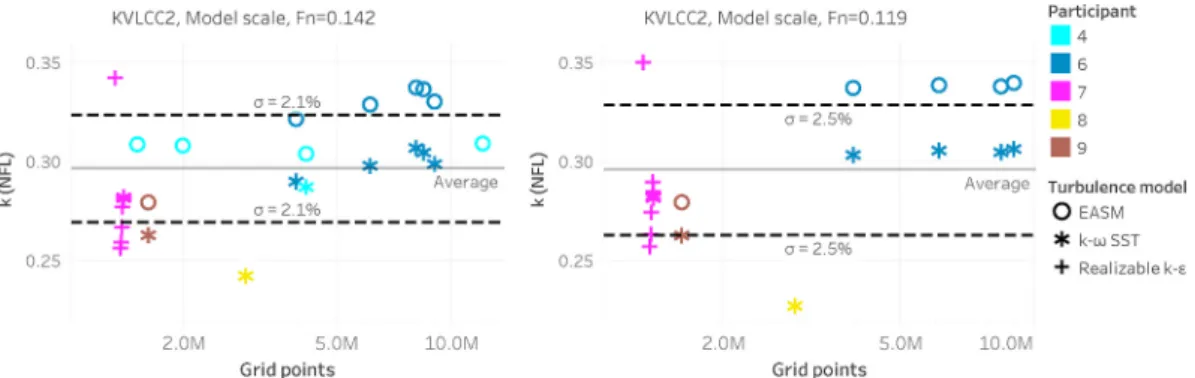
Form factors with numerical friction lines for KVLCC2 are presented in Fig. 13. Opposing to the results from the ITTC-57 line, the mean value of the form factors with NFL are almost identical for both speeds. Close investigation on the individual simulation points between the different speeds also support this suggestion except the simulations from Strath-clyde (Participant 8) and the coarse grids of SSPA/CTU (Participant 6). KVLCC2 in both loading conditions shows smaller speed dependency with ITTC-57 line compared to KCS as the Reynolds number difference between the two speeds is smaller. It is worth noticing that the speed dependency is larger in design condition than the ballast loading con-dition with the ITTC-57 line. This is a consequence of the “artificial” steepness of the ITTC-57 line which increases as the Re decreases. Therefore, as any other model with big scale factor (the ratio of ship to model length) would, KVLCC2 model in design condition suffers more from the scale effects with the ITTC-57 line.
The standard deviations of the form factor in percentage of (1 +k) predictions for all cases are presented in Table 9. Using the Katsui line, the standard deviation of the form factor are the same in all cases compared to using the ITTC-57 line as the same computations were used. Form factors with NFL showed an increase in the standard deviation for the KVLCC2 in design condition. However, the standard deviation is reduced significantly for KVLCC2 in ballast loading condition and especially for KCS due to a decrease in variation of form factors obtained from different turbulence models. Even though the dependence of tur-bulence models on form factor seems to decrease by the adoption the NFL of the same code and turbulence model as the double body simu-lation, the form factors are not expected to be the same for different turbulence models. Application of NFL for different turbulence models arranges the quantity of form resistance with respect to the friction line of the respective turbulence model. As a result, nearly the same full scale viscous resistance values can be obtained by the different turbulence models as shown in Section 5.4.2.
As an alternative to the CFD based form factor determination method used in this study, Wang et al. (2016) and Terziev et al. (2019) calcu-lated the form factors simply by dividing the viscous pressure coefficient to friction coefficient (k = CPV/CF) obtained from the double body
simulation with the hull. Therefore, the need of any friction line is removed for form factor determination. This method of form factor determination is dismissed in this study because of the deviation from the approach of Hughes (1954) as CF from double body computation
already includes the additional skin friction caused by the curvature effects which should have been included the form resistance as explained in Section 2.
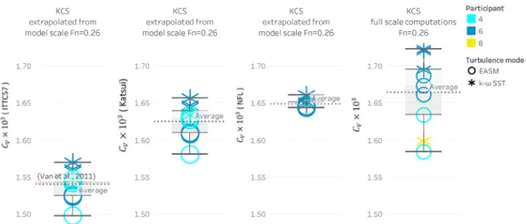
5.4. Full scale predictions
5.4.1. Statics of computed CF and CPV in full scale
Full scale double body simulations are performed according to the conditions described in Table 2. The friction and viscous pressure resistance coefficients are presented in Fig. 14 and Fig. 15, respectively.
Table 9
Statistics of the form factor predictions with ITTC-57 line (I), Katsui line (K) and numerical friction lines (N).
Quantity KVLCC2 (design) KVLCC2 (ballast) KCS (design) Fn 0.119 Fn 0.142 Fn 0.119 Fn 0.142 Fn 0.152 Fn 0.260 Mean (I) 0.212 0.223 0.175 0.181 0.102 0.117 Mean (K) 0.271 0.280 0.227 0.231 0.149 0.156 Mean (N) 0.296 0.296 0.242 0.243 0.163 0.165 σ (I) 1.5% 1.6% 2.1% 2.0% 1.3% 1.2% σ (K) 1.5% 1.6% 2.1% 2.0% 1.3% 1.2% σ (N) 2.4% 2.1% 1.8% 1.9% 0.7% 0.8%
The mean and standard deviation of the computed resistance co-efficients are calculated excluding the results from NRC-OCREand SSSRI who encountered difficulties with grid generation. The mean of CF is by
approximately 6% and 3% higher than the Katsui line due to additional skin friction caused by the curvature effects for KVLCC2 and KCS, respectively. The standard deviation of CF in full scale is reduced
considerably compared to model scale for KVLCC2 at both loading conditions mainly because of the reduction of dependence on turbulence models. The standard deviation of CF is similar both in model and full
scale for the KCS hull. However, the standard deviation of CPV is
increased for KCS and KVLCC2 in design condition compared to model scale while the variation of CPV is similar in model and full scale for
KVLCC2 in ballast condition. Considering the standard deviation and the quantity of CF and CPV observed in full scale simulations, the viscous
pressure resistance component is the dominant source of variation in CV.
As mentioned earlier, the difficulties in the grid generation for NRC- OCRE and SSSRI can be observed through the average y+values varied
between 450 and 750 for NRC-OCRE and 8300 to 15,000 for SSSRI. As a result, mainly the predicted CF values are significantly higher than the
mean of the rest of the computations. A strong dependence on
Fig. 14. Full scale CFD simulations. Computed frictional coefficient, CF, for KVLCC2 hull in design loading condition at Fn = 0.142 (left), KVLCC2 in ballast loading condition Fn = 0.142 (center) and KCS hull in design loading condition at Fn = 0.26 (right).
Fig. 15. Full scale CFD simulations. Computed viscous pressure coefficient, CF, for KVLCC2 hull in design loading condition at Fn = 0.142 (left), KVLCC2 in ballast loading condition Fn = 0.142 (center) and KCS hull in design loading condition at Fn = 0.26 (right).