HAL Id: hal-01061701
https://hal-enpc.archives-ouvertes.fr/hal-01061701
Submitted on 8 Sep 2014
HAL is a multi-disciplinary open access
archive for the deposit and dissemination of
sci-entific research documents, whether they are
pub-lished or not. The documents may come from
teaching and research institutions in France or
abroad, or from public or private research centers.
L’archive ouverte pluridisciplinaire HAL, est
destinée au dépôt et à la diffusion de documents
scientifiques de niveau recherche, publiés ou non,
émanant des établissements d’enseignement et de
recherche français ou étrangers, des laboratoires
publics ou privés.
Upper Bounding in Inner Regions for Global
Optimization under Inequality Constraints
Ignacio Araya, Gilles Trombettoni, Bertrand Neveu, Gilles Chabert
To cite this version:
Ignacio Araya, Gilles Trombettoni, Bertrand Neveu, Gilles Chabert. Upper Bounding in Inner Regions
for Global Optimization under Inequality Constraints. Journal of Global Optimization, Springer
Verlag, 2014, 60 (2), pp.145-164. �10.1007/s10898-014-0145-7�. �hal-01061701�
(will be inserted by the editor)
Upper Bounding in Inner Regions for Global
Optimization under Inequality Constraints
Ignacio Araya · Gilles Trombettoni · Bertrand Neveu · Gilles Chabert
Received: date / Accepted: date
Abstract In deterministic continuous constrained global optimization, upper bounding the objective function generally resorts to local minimization at several nodes/iterations of the branch and bound. We propose in this paper an alternative approach when the constraints are inequalities and the feasible space has a non-null volume. First, we extract an inner region, i.e., an entirely feasible convex polyhedron or box in which all points satisfy the constraints. Second, we select a point inside the extracted inner region and update the upper bound with its cost. We describe in this paper two original inner region extraction algorithms implemented in our interval B&B called IbexOpt [27]. They apply to nonconvex constraints involving mathematical operators like +, q, /, power, sqrt, exp, log, sin. This upper bounding shows very good performance obtained on medium-sized systems proposed in the COCONUT suite.
Keywords Global optimization · Upper bounding · Intervals · Branch and bound · Inner regions · Interval Taylor
Ignacio Araya is supported by the Fondecyt Project 11121366 and the UTFSM Researcher Associated Program.
I. Araya
UTFSM, Universitad Federico Santa Maria, Valparaiso, Chile E-mail: [email protected]
G. Trombettoni
IRIT, LIRMM, Universit´e Montpellier 2, France E-mail: [email protected]
B. Neveu
Imagine LIGM Universit´e Paris–Est, France E-mail: [email protected]
G. Chabert
LINA, Ecole de Mines de Nantes, France E-mail: [email protected]
1 Introduction
In deterministic constrained global optimization, upper bounding the objec-tive function consists in finding a feasible point that improves the best cost already found in the branch and bound. Most global optimizers resort to lo-cal minimization1 using a Lagrangian relaxation. The considered function is
sometimes big, which may render the local minimization slow.
This paper describes an alternative approach for constrained global opti-mization. This approach avoids the cost of evaluating the objective function repeatidly. It however requires the feasible space formed by the inequality constraints to have a non-null volume. More precisely, the continuous global optimization problem we handle is defined by:
min
x∈[x]f (x) subject to g(x) ≤ 0,
where f : Rn→ R is the real-valued objective function and g : Rn → Rmis a
vector-valued function. x = (x1, ..., xi, ...xn) is a vector of variables varying in
a box [x].2 x is said to be feasible if it satisfies the constraints.
The main idea is to exploit so-called inner regions, i.e., subsets of the search space in which all points are feasible.
Two communities working on interval methods have proposed several heuris-tics for checking whether a given domain is an inner box or, more interestingly, extracting inner boxes inside a given domain (outer box). The interval (nu-merical) analysis community has especially studied linear systems with inter-val coefficients [24, 25]. The constraint programming community has proposed general-purpose heuristics for non convex systems of inequality constraints [9, 4, 10].
Two original inner region extraction algorithms are described in this paper. These heuristics are applied for the first time to general-purpose constrained global optimization. At every node (iteration) of our interval B&B named IbexOpt[27], the cost is bounded above by using two inner region extraction heuristics called InnerPolytope and InHC4.
The InnerPolytope algorithm, described in Section 3, builds a hyperplane for every inequality constraint. The hyperplane is produced by a special convex form of interval Taylor where the expansion point is chosen at a corner of the studied outer box. If it succeeds in building an inner polytope, the point minimizing an over-estimated linearized form of the objective function is used to update the upper bound.
InHC4 is a completely different approach that makes no linearization. On the other hand, the inner region has a more basic shape, namely a box. It is based on an operator-wise decomposition of each function and is described in Section 4. It first tries to extract an inner box from the current outer box constraint per constraint. If it fails, it simply picks a point randomly inside
1 We consider minimization in this paper without loss of generality. 2 An interval [x
i] = [xi, xi] defines the set of reals xi s.t. xi≤ xi≤ xi. A box [x] is the
the outer box and checks its feasibility. If it succeeds, a simple monotonicity analysis of f replaces the intervals of the monotonic variables by the adequate bounds in the found inner box and the other values are randomly chosen (no additional feasibility check is necessary since all the points in the box returned by InHC4 are feasible). The feasible point thus obtained is used to update the upper bound.
Contrary to existing approaches, the proposed inner region extraction algo-rithms separate the feasibility part (handled first, by inner region extraction) and the computation of the cost (handled next, inside the found inner region). Section 5 highlights that, like the other inner region extraction algorithms, our algorithms are heuristics. In other words, they sometimes fail to find an in-ner region even if one such region exists. However, the same section underlines that they are rather inexpensive.
The experiments shown in Section 6 highlight that this upper bounding policy, with the two procedures InnerPolytope and InHC4, brings very good speedups to our interval B&B IbexOpt [27].
2 Background and handled problem
Intervals allow reliable computations on computers by managing floating-point bounds and outward rounding.
Intervals
An interval [xi] = [xi, xi] defines the set of reals xi s.t. xi≤ xi≤ xi, where
xi and xi are floating-point numbers. IR denotes the set of all intervals. The
size or width of [xi] is w([xi]) = xi− xi. A box [x] is the Cartesian product
of intervals [x1] × ... × [xi] × ... × [xn]. Its width is defined by maxiw([xi]).
m([x]) denotes the middle of [x]. The hull of a subset S of Rn is the smallest
n-dimensional box enclosing S.
Interval arithmetic [20] has been defined to extend to IR elementary func-tions over R. For instance, the interval sum is defined by [x1] + [x2] = [x1+
x2, x1+ x2]. When a function f is a composition of elementary functions, an
extension of f to intervals must be defined to ensure a conservative image computation.
Definition 1 (Extension of a function to IR; inclusion function; range enclosure)
Consider a function f : Rn→ R.
[f ] : IRn → IR is said to be an extension of f to intervals iff: ∀[x] ∈ IRn [f ]([x]) ⊇ {f (x), x ∈ [x]} ∀x ∈ Rn f (x) = [f ]([x, x])
The natural extension [f ]N of a real function f corresponds to the mapping
of f to intervals using interval arithmetic. The inner interval linearizations proposed in this paper is related to the first-order interval Taylor exten-sion [20], defined as follows:
[f ]T([x]) = f (˜x) +
X
i
[ai] . ([xi] − ˜xi)
where ˜x denotes any point in [x], e.g., m([x]), and [ai] denotes
h ∂f ∂xi i N([x]). Equivalently, we have: ∀x ∈ [x], [f ]T([x]) ≤ f (x) ≤ [f ]T([x]).
Example. Consider f (x1, x2) = 3x21+ x22+ x1x2 in the box [x] = [−1, 3] ×
[−1, 5]. The natural evaluation provides: [f ]N([x1], [x2]) = 3[−1, 3]2+[−1, 5]2+
[−1, 3][−1, 5] = [0, 27] + [0, 25] + [−5, 15] = [−5, 67]. The partial derivatives are: ∂x∂f 1(x1, x2) = 6x1+ x2, [ ∂f ∂x1]N([−1, 3], [−1, 5]) = [−7, 23], ∂f ∂x2(x1, x2) = x1+ 2x2, [∂x∂f
2]N([x1], [x2]) = [−3, 13]. The interval Taylor evaluation with ˜x =
m([x]) = (1, 2) yields: [f ]T([x1], [x2]) = 9 + [−7, 23][−2, 2] + [−3, 13][−3, 3] =
[−76, 94].
Handled problem
A continuous constrained global optimization problem is defined as follows. Definition 2 (Constrained global optimization)
Consider a vector of variables x = (x1, ..., xi, ...xn) varying in a box [x], a
real-valued function f : Rn → R, vector-valued functions g : Rn → Rm and
h : Rn→ Rp.
Given the system S = (f, g, h, [x]), the constrained global optimization prob-lem consists in finding:
min
x∈[x]f (x) subject to g(x) ≤ 0 ∧ h(x) = 0.
f denotes the objective function; g and h are inequality and equality con-straints respectively. x is said to be feasible if it satisfies the concon-straints.
Our interval optimizer extracts inner boxes and inner polytopes inside clas-sical (outer) boxes.
Definition 3 Consider a system (f, g, [x]) comprising only inequality con-straints. An inner region rinis a feasible subset of [x], i.e., rin⊂ [x] and all
points x ∈ rin satisfy g(x) ≤ 0.
Only a few softwares rigorously solve the constrained global optimization defined above. Several global optimizers based on an interval B&B, like Glob-Sol [12] and Icos [14], return a tiny box guaranteed to contain a real-valued vector x ǫ-minimizing: f (x) s.t. g(x) ≤ 0 ∧ h(x) = 0.3
3 ǫ-minimize f (x) means minimize f (x) with a precision ǫ, i.e., we have f (y) ≥ f (x) − ǫ,
Inspired by the IBBA solver [22], we propose to relax pure equalities hj(x) = 0 by “thick” equations hj(x) ∈ [−ǫeq, +ǫeq], i.e., two inequalities:
−ǫeq≤ hj(x) ≤ +ǫeq. Therefore, our IbexOpt global optimizer [27] rigorously
computes a floating-point vector x ǫ-minimizing:
f (x) s.t. g(x) ≤ 0 ∧ (−ǫeq≤ h(x) ≤ +ǫeq).
Note that IBBA and IbexOpt can only guarantee the global optimum of the relaxed system, although ǫeq can often be chosen almost arbitrarily small.
Also note that most of the deterministic global optimizers (generally based on a spatial branch and bound), like Baron [26] or Couenne [3], can guarantee the solution neither to the constrained global optimization problem (Definition 2) nor to the relaxed problem. Finally note that, in practice, most of the equations are already “thick” and thus do not need to be further relaxed with an ǫeq.
Equations modeling physical systems often have indeed at least one coefficient that can be represented by an interval constant. This parameter corresponds to a bounded uncertainty, e.g., an imprecision on a measurement.
In the sake of simplicity, since our optimizer accepts inequalities and re-laxed equalities that are also inequalities, we consider from now on that the handled constrained global optimization problem is:
min
x∈[x]f (x) s.t. g(x) ≤ 0,
i.e., the functions h(x) − ǫeq(≤ 0) and −h(x) − ǫeq(≤ 0) belong to the vector
g : Rn→ Rmof functions.
Note that numerous convex and nonconvex mathematical operators can be taken into account, such as +, q , /, xn, exp, log, sqrt, sine, etc.
3 Inner polytope algorithm
The main idea is to build a half-space for each inequality gj(x) ≤ 0, such that
all the points in the computed half-space satisfy the constraint. For that pur-pose, we use a specific first order interval Taylor form of a nonlinear function. The usual first-order interval Taylor form, defined in Section 2, can select any expansion point ˜x inside the box to achieve the linearization. Instead of the usual midpoint, a corner of the box is chosen here, i.e., x.
Consider a function gj: Rn→ R and a domain [x]. For any variable xi∈ x,
let [aji] be h∂gj ∂xi
i
N([x]). The idea is to bound gj(x) from above with an affine
function gl
j(x) obtained by a corner-based interval Taylor form. For all real
vector x ∈ [x], we have:
gj(x) ≤ gjl(x) = gj(x) +
X
i
aji.(xi− xi). (1)
If we consider an inequality gj(x) ≤ 0, relation (1) enables us to build a
hyper-plane gl
gl
j(x) ≤ 0. That is to say, the linear function gjl(x) can be used to define an
inner region of [x].
Proposition 1 The interval linear form (1) is correct and rigorous, i.e., it can be made robust to computation errors over floating-point numbers. Rigor is ensured by the interval Taylor [21]. The correction of relation (1) lies on the fact that any “variable” (xi− xi) is positive since its domain is [0, di],
with di= w([xi]) = xi− xi. Therefore, maximizing each term [aji].(xi− xi) for
any point (xi− xi) ∈ [0, di] is obtained with aji.
Example
Consider the constraint
g1(x1, x2) = x31+ cos(x1) − sin(x2) − 0.15 ≤ 0
in a box [x1] × [x2] = [−0.32, 0.52] × [0.90, 1.06].
We can derive from the gradient of g1:
– h∂g1 ∂x1 i N = 3.[−0.32, 0.52] 2−sin([−0.32, 0.52]) = 3[0, 0.2704]−[−0.314, 0.497] = [−0.497, 1.1252] – h∂g1 ∂x2 i N = −cos([0.90, 1.06]) = [−0.6216, −0.488872082]
The function g1 is illustrated in Fig. 1. The feasible space appears in grey.
Applying (1) to g1provides:
g1(−0.32, 0.90) + 1.1252 (x1+ 0.32) + −0.4889 (x2− 0.90) ≤ 0.
The left part of the figure shows in dark grey the corresponding inner region, a polytope obtained by intersecting this half-space with the box.
The right side of the figure shows an inner space computed by a standard interval Taylor with an expansion point taken in the middle of the box:
g1(0.10, 0.98) + [−0.497, 1.1252] (x1− 0.10) + [−0.6216, −0.4889] (x2− 0.98)
This form implies a (non necessarily convex) union of four polytopes, each polytope being obtained by the intersection of 5 half-spaces: the first two correspond to the sign constraints (a shifted orthant, separated by dotted lines on the figure), the next two correspond to the box boundaries and the last to the Taylor expansion. For instance, the first polyhedron is:
x1< m[x1] x2< m[x2] x1≥ x1 x2≥ x2 0.0155067948 − 0.497 (x1− 0.10) − 0.6216 (x2− 0.98) ≤ 0
Note that two of the polytopes are empty on this example (including the one detailed above). The other two appear on the figure and are generated by the following Taylor forms:
1. 0.0155067948 − 0.497 (x1− 0.10) − 0.4889 (x2− 0.98) ≤ 0 (x1< m[x1] and x2> m[x2]) 2. 0.0155067948 + 1.1252 (x1− 0.10) − 0.4889 (x2− 0.98) ≤ 0 (x1> m[x1] and x2> m[x2]) 0.3 -0.2 -0.1 0 0.1 0.2 0.3 0.4 0.5 1.06 1.02 0.98 0.94 0.90 x1 x2 0.3 -0.2 -0.1 0 0.1 0.2 0.3 0.4 0.5 1.06 1.02 0.98 0.94 0.90 x1 x2
Fig. 1 Left: Inner polytope generated by a corner-based interval Taylor in (x1, x2).
Right:Two inner polytopes generated by a midpoint interval Taylor in two of the four orthants.
A linear program for a better feasible point (upper bound)
Applying this idea to the objective function f (x) and to the inequalities gj(x) ≤ 0, we can derive the linear program LPub:
LPub= min f (x) +P iai∗ (xi− xi) subject to : ∀j gj(x) +Pia j i ∗ (xi− xi) ≤ 0 ∀i xi ≤ xi∧ xi≤ xi
A Simplex algorithm solves LPub and returns infeasibility or the optimal
so-lution xl(see Algorithm 1). Infeasibility proves nothing because the linearized
system is more constrained than the original system, so that one could still find solutions in the original one. If the Simplex algorithm returns an optimal solution of the inner approximation, then xl is also a solution to the
origi-nal system, maybe not the optimal one. The previous process is correct on
Algorithm 1 InnerPolytopeUB (in: S, [x]out; in-out: ub, x ub)
LPub← InnerLinearization (S, [x]out)
xl← Simplex(LPub)
if xl6= ⊥ and FeasibilityCheck(xl, S) then
cost← [f ]N([xl, xl])
if cost < ub then ub← cost; xub← xl end if
the real numbers, but is not necessarily always correct on a computer due to roundoff errors on floating-point numbers. Indeed, since we use a standard Simplex algorithm working with floating-point numbers, it is possible that the best (floating) value returned by the LP solver falls slightly outside the inner polytope and is not feasible. That is why we render the whole process rigor-ous by checking the feasibility of x with an interval evaluation (see line 3 of Algorithm 1).
The pseudocode finally details that one evaluates the objective function (the original one, not the linearized one) at the point xl and potentially
im-proves the upper bound. In this case, we update the point xub and its cost
(i.e., the new upper bound) ub.
Related work, discussion
Interval Taylor forms have often been used to produce an outer linear approx-imation of the solution set or of the objective function. However, when the expansion point is chosen strictly inside the domain, the system obtained by an interval Taylor form is not convex. It forms an intersection of non-convex sub-spaces. (Examples can be found in [21, 12, 19].) Contracting optimally a box containing this non-convex relaxation has been proven to be NP-hard [13]. This explains why the interval analysis community has worked a lot on this problem for decades [23, 11, 6].
Several researchers proposed to select as expansion point of the interval Taylor form a corner of the studied box, instead of the usual midpoint [2, 15–17, 21]. The main drawback is that it leads generally to a larger system relaxation surface. The main virtue is that the approximated solution set belongs to a unique orthant and is convex, i.e., it is a polytope.
The dual form defined by (1) has never been used before to achieve an inner polytope extraction, and so has never been used before to improve an upper bound in constrained global optimization.
4 The InHC4 algorithm
InHC4is similar to the state-of-the-art constraint propagation algorithm HC4 [4, 9, 18] to the extent that its core procedure called InHC4-Revise (in short InHC4R) is based on a forward-backward traversal of the tree representation of constraints (see Fig. 2). Furthermore, the forward phase is exactly the same as in the core procedure of HC4, called HC4-Revise (in short HC4R). However, the main loop and the backward phase are radically different, as we detail below. In addition, they do not calculate of course the same box. Let us start with the main loop.
The main loop of InHC4 handles every constraint once in sequence and performs each time a call to InHC4R. Given an input box [x], InHC4R produces an inner box [x]in ⊆ [x] with respect to the constraint under process. It is
then easy to build incrementally a box that is inner with respect to the whole system. More precisely, the main loop:
– calls InHC4R on the 1st constraint with the outer box as input,
– calls InHC4R on the jthconstraint with the box obtained after the previous
call (the one for the (j − 1)thconstraint), provided it is non empty.
Thus, if a non empty box is returned after the handling of the last con-straint, then this box is inner w.r.t. all the constraints.
Let us now detail InHC4R. Unlike the refutation process of HC4R, InHC4R tries to extract an inner region at each operator of the constraint.
Fig. 2 Binary tree representation of the constraint 10y − x − y2 ≤ 0. Left: First forward
evaluation phase. Right: backward inner projection phase.
Let us denote by [x] the input box and gj(x) ≤ 0 the constraint. Each node
of the tree is associated to an interval, the intervals related to the leaves are initialized with the corresponding values in [x]. Then, the following two phases are performed:
– Forward evaluation (see Fig. 2–left): The tree is traversed from the leaves to the root and intervals associated to an operator are computed with interval arithmetics. For example, the node pointed by the arrow is initialized with the interval [0, 10] − [0, 15] = [−15, 10]. Thus, every node contains an inter-val corresponding to the natural interinter-val einter-valuation of the subexpression. – Backward inner projection (see Fig. 2–right): From the root to the leaves,
the intervals in each node are contracted using specific inner projection operators.
In each node related to a binary operator op and labeled with an interval [z] (i.e., z = x1op x2), the 2-dimensional box corresponding to its children
vertices x1 and x2 is reduced to an inner box [x1]in× [x2]in such that:
If op corresponds to a unary operator (i.e., z = op(x)), its unique child is reduced to [x]in, such that:
∀x ∈ [x]in: op(x) ∈ [z] (3)
If an inner projection returns an empty box (i.e., no box satisfying (2) or (3) has been found), then the top-down process is interrupted. It means that InHC4Rfailed to find a box that is inner w.r.t. gj(x) ≤ 0. It implies that InHC4
failed to find a box that is inner w.r.t. the n inequality constraints, so that the main loop of InHC4 is interrupted.
Consider for instance the backward projection applied to the product op-erator of Fig. 2–right and its two children. The reduced intervals appear in bold in the left side of each node (e.g., [z] is [0, 5]). Before reduction, its chil-dren are labeled with the intervals [10, 10] and [0, 1]. They are then reduced to [10, 10] and [0, 0.5] respectively. The reduction agrees with relation (2), i.e, ∀y ∈ [0, 0.5] : 10 . y ∈ [0, 5]. The next section details how these basic inner projection operators are achieved.
4.1 Inner projection for basic operators
We report in this section the main guidelines to implement the inner projection for the main mathematical operators. Four different cases must be studied and follow a monotonocity analysis. This approach extends the case-by-case approach proposed in Section 3 of [7]. We have built a more generic projection based on monotonicity properties.4The first case is trivial but serves as a basis
for understanding the others. Case 1: monotonic unary operators
The first case applies to monotonic and continous unary operators, like log and exp. More precisely, we consider operators z = op(x) that are continuous and monotonic w.r.t. x in [x].
In this case, inner projection is trivial (see Fig. 3). We compute the max-imum inner interval (i.e, no feasible point is lost, leaving aside roundoffs) using the inverse function of op, like in a standard projection in HC4R. E.g., if z = exp(x), [x]in := log([z]). However, to take into account floating-point
roundoff errors, the outward rounding of HC4R is replaced by inward rounding.5
4 In addition, Chabert & Beldiceanu handled a dual problem consisting in finding a box
with no solution (i.e., all points in this box violate the constraints) and required an initial point to be “inflated” to a box...
5 With floating-point numbers, an interval evaluation is conservative (i.e., contains all
the real-valued images) if the lower bound of the interval image is rounded towards −∞ while the upper bound is rounded to +∞. Both rounding operations constitute a so-called outward rounding.
x z=op(x)
z
Fig. 3 Case 1: Inner projection of a monotonic operator. The horizontal segment in the bottom of the figure is the result of the inner projection on x.
Case 2: non monotonic unary operators
The second case applies to non monotonic unary operators, like x2 or sine.
More precisely, we consider operators z = op(x) that are not monotonic w.r.t. x in [x].
In this case, we achieve a piecewise monotonicity analysis and obtain an interval for every monotonic part. Finally, unless the union of computed in-tervals forms a connected set, we select randomly one interval. Note that for
x z=op(x)
z
Fig. 4 Case 2: Inner projection of a non monotonic operator, i.e., sqr. Two intervals (il-lustrated by horizontal segments) are obtained by projection on x (i.e., using the inverse operation of sqr), and one of them is randomly chosen and returned.
With inward rounding, the lower bound is rounded towards +∞ and the upper bound towards −∞. The property enforced by outward (resp. inward) rounding for an operator op is (1), resp. (2):
1. ∀x ∈ [x] ∃z ∈ op([x]) z = op(x) 2. ∀z ∈ op([x]) ∃x ∈ [x] z = op(x)
non monotonic unary operators, the standard HC4R returns the hull of the in-tervals. For an inner projection in InHC4R, only a single interval is kept since holes between these intervals represent inconsistent/infeasible points (Fig. 4). Case 3: monotonic binary operators
A specific handling must be carried out on monotonic binary operators. Definition 4 A function R2 → R f(x
1, x2) is nondecreasing (resp.,
non-increasing) monotonic w.r.t. x1 in [x1] × [x2] if for all c in [x2] we have:
∀(a, b) ∈ [x1]2, a ≤ b ⇒ f (a, c) ≤ f (b, c) (resp. a ≤ b ⇒ f (a, c) ≥ f (b, c)).
f (x1, x2) is said monotonic if f (x1, x2) is monotonic w.r.t each of its
vari-ables in [x1] × [x2].
Note that f may be for instance nondecreasing w.r.t. x1and nonincreasing
w.r.t. x2.
For binary (or n-ary) operators that are monotonic w.r.t. each of their vari-ables, a generic procedure, called MonoMaxInnerBox, can compute randomly one maximal inner box, if one such box exists, as shown in Fig. 5.
x1 x2 g(x1 ,x2 )= 0 (x
. .
1,x2) x1 x.
2.
[z] other maximal inner boxesFig. 5 Case 3, procedure MonoMaxInnerBox: The dotted box corresponds to a maximal inner box of [z] w.r.t. the monotonic constraint g(x1, x2) ≤ 0. A point ˙x1 is randomly
picked inside the range of allowed values illustrated by the horizontal segment. Only one remaining value ˙x2 can then make the computed inner box maximal.
As depicted in Fig. 5, there usually exists an infinite number of maximal boxes so that we select randomly one of these maximal inner boxes.
Handling a monotonic binary operator amounts to handling the two in-equalities
z ≤ (x1 op x2) ≤ z.
Both inequalities are handled in sequence, the inner box computed for one inequality being used as input of the second one. This procedure is of course used for implementing the inner projection of the addition and subtraction operators.
It is also used for handling several (monotonic) subcases of the non mono-tonic binary operators: the multiplication and the division described below. Case 4: non monotonic binary operators
The last case includes the binary (or n-ary) operators that are not monotonic w.r.t. each of their variables, i.e., the multiplication and the division.
Fig. 6 illustrates the two main cases for the multiplication x1.x2 ∈ [z],
depending whether 0 belongs or not to [z].
x1.x2 >z maximal innerbox w.r.t. x1.x2∈ [z] x1 x2 x2 x1 0 ∈ [z] 0 ∉ [z] x1.x2<z [x]:=hull([xA],[xB]) [xA] x2 [xB] x1
Fig. 6 Inner projection for the binary multiplication. Left: Two maximal boxes that can indifferently be computed by MonoMaxInnerBox in the two disjoint inner regions (quadrants) defined by the operator x1.x2 ∈ [z] ≥ 0. Middle and right: Maximal box computed for
x1.x2∈ [z] ∋ 0 (z ≥ −z) with four calls to MonoMaxInnerBox (boxes in grey).
For the case x1.x2 ∈ [z] ∋ 0, note that a direct procedure (although more
difficult to be implemented) could also been achieved without resorting to MonoMaxInnerBox.
Two different implementations for the division have been tested. One ap-proach amounts to rewriting x1/x2= x1.x1
2 ∈ [z]. The other approach directly
considers the different monotonic subcases of the operator, like for the muli-plication. Non exhaustive experiments show that both versions seem to have the same performance in practice.
4.2 Improving the upper bound using InHC4
Algorithm 2 details how InHC4 is used by IbexOpt for improving the upper bound.
Algorithm 2 Inhc4UB (in: S, [x]out; in-out: ub, x ub)
[x]in← InHC4 (S, [x]out) /* Inner box extraction */
if [x]in6= ∅ then
[x]in← MonotonicityAnalysis (f , [x]in)
x← RandomProbing([x]in) // or gradient descent
else
x← RandomProbing([x]out)
end if
cost← [f ]N([x, x]) /* Cost evaluation */
if cost < ub and ([x]in6= ∅ or [g]
N([x, x]) ≤ 0) then
ub← cost; xub← x
end if
If an inner box [x]in is found by InHC4, then MonotonicityAnalysis
an-alyzes the monotonicity of the objective function f w.r.t. every variable xi.
If the partial derivative [ai] =
h ∂f ∂xi i N([x] in) ≥ 0, then f is increasing w.r.t.
xi in [x], and [xi] is replaced by the degenerated interval [xi, xi] in [x]in for
minimizing f (x) over [x]in. If [a
i] ≤ 0, f is decreasing and [xi] is replaced by
[xi, xi] in [x]in.
Next, we pick randomly a point x inside the resulting box, and replace xub
by x if x satisfies the constraints and improves the best cost ub. Two different cases may occur. If an inner box has been extracted by InHC4, then a point is selected inside [x]in. The feasibility of x does not need to be checked since [x]in
contains only feasible points. If no inner box is available, a random point is still picked in the outer box [x]out, and the constraints must then be checked.
Replacing this simple probing by a home-made gradient descent did not improve the strategy. However, our implementation was not sophisticated and we should try other descent algorithms (quasi-Newton, etc.) before drawing definite conclusions.
5 Properties
Several properties can be deduced from the material presented in the previous two sections. The first one is a negative one.
Observation 1 The two algorithms InnerPolytope and InHC4 are correct but incomplete, i.e., they are heuristics that can sometimes miss an inner region whereas one such region does exist.
InnerPolytopeis incomplete because it does not calculate, in general, an inner polytope that is maximal (with respect to the inclusion), eventhough roundoff errors are left aside. The calculated polytope may be empty. This is a consequence of the overestimate produced by the interval Taylor form.
The InHC4-Revise procedure (handling a single constraint) is also incom-plete because it overestimates the intervals in the forward phase and makes random choices in the backward phase. Indeed, if an intermediary node is
overestimated, we can choose in the backward phase a part of the domain that is not compatible with the variables. The overestimate can be induced by variables appearing several times in the function or by a discontinuity of the function. Consider for instance the constraint sin(1/x) ≤ 0.5 and the domain [x] = [−1/π, 1/π]. During the forward phase, the discontinuity of 1/x leads to hull [−∞, −π] ∪ [π, +∞] to [−∞, +∞]. During the backward phase, choosing unluckily the monotonic part [−π/2, π/6] would lead to find no inner box.
Finally, even though InHC4-Revise was complete (for a single constraint), the InHC4 algorithm could be not able to find a box that is inner to the whole system. One can observe that all the cases handled by the InHC4R procedure, except the first one (monotonic unary operator), ignore a part of the feasible space.6 Therefore, an inner box “arbitrarily” built by InHC4R for a given
con-straint, as underlined in Section 4.1, sometimes leads to an empty inner box when handling a subsequent constraint.
The following proposition highlights an interesting aspect of InHC4-Revise. Proposition 2 Consider a function gj that contains at most one occurrence
of each variable and is continuous in its domain [x].
InHC4-Revise always succeeds in extracting an inner box [x]in w.r.t. the
constraint gj(x) ≤ 0 in the domain [x], and [x]in is maximal (leaving aside
roundoff errors due to floating-point arithmetic), i.e., there is no other larger box [x]in′
⊃ [x]in that is an inner box of [x] w.r.t. g j.
Proof (sketch)
As mentioned above, the continuity of the function gjand the single occurrence
condition are the conditions to avoid an overestimate of the basic operators during the forward phase.
We can prove that every implemented unary and binary operator computes a maximal inner box, leaving aside the loss involved by inward roundoffs. This is straightforward for cases 1 and 2. This is obtained by construction in the case 3 from the procedure MonoMaxInnerBox. The only difficulty lies in the proof of the case x1.x2∈ [z] when 0 ∈ [z].7
The single occurrence condition follows that of the standard HC4R [5]. It ensures that the expression is a tree structure and not a directed acyclic graph (because a variable appearing several times in the expression has several par-ents in the graph) that cannot keep the property by induction. In other terms, the condition ensures that, during the backward traversal, the composition of inner boxes provides maximal inner intervals on all the dimensions. ✷
6 In the case 2, only one inner interval is considered among the different ones in the union.
In the case 3, only one maximal inner box is computed (using a random choice on x1) among
an infinite number of possibles boxes. The last case gathers both drawbacks (from cases 2 and 3). Consider for instance the case of the multiplication x1.x2∈ [z] where z is positive
(see left side of Fig. 6).
7 The difficulty is only related to our implementation. The maximality can be more easily
We recall that the maximality property does not hold for a system of in-equality constraints handled by InHC4. Also note that InnerPolytope and InHC4 are not comparable because the box produced by InHC4 is not neces-sarily included in the polytope produced by InnerPolytope.
A second proposition provides the worst-case time-complexity of our two inner region extraction algorithms.
Proposition 3 Consider a system (f, g, [x]) with n variables and m inequali-ties. Let k be the maximum number of unary and binary operators in a function gj. Let t the maximum time required to evaluate a primitive mathematical
op-erator.
Then, the worst-time complexity of the InnerPolytope extraction proce-dure is O(m(k.t + n)). The worst-time complexity of the InHC4 extraction procedure is O(m.k.t).
Proof
For InnerPolytope, computing a hyperplane (or generating a linearized form of the objective function) is achieved in time O(k.t+n). Indeed, computing the gradient of a given function gj is obtained in time O(k.t + n) with automatic
differentiation; evaluating gj(x) requires time O(k.t); the sum of terms aji.(xi−
xi) is O(n) for all the variables. Finally, generating the linear program LPub
amounts to m + 1 calls to the previous procedure (i.e., the m constraints plus the objective function). Note that the time complexity for a call to an LP solver must be added to this time complexity in the procedure InnerPolytopeUB.
The procedure InHC4 handles at most m constraints one by one. The proce-dure InHC4R applies at most k interval evaluations in time O(t) each during the backward projection phase, and k times a constant number (between one and four) calls to the procedure MonoMaxInnerBox during the top-down projection phase. When applied to a binary basic monotonic mathematical operator, the complexity of MonoMaxInnerBox is O(t) because it amounts to two iterations (on the two variables), each dominated by an interval evaluation of the basic operator. ✷
In contrast to InnerPolytope, observe that the worst-case complexity of InHC4is not reached when InHC4R fails to handle a constraint, since the loop on all the constraints is then interrupted. Therefore, the less chances InHC4 has to extract an inner box (because the outer box is large compared to the inner subspace), the fewer constraints are handled by InHC4, and the shorter is the runtime needed.
6 Experiments
These two upper bounding algorithms have been implemented in our interval B&B IbexOpt. IbexOpt [27] is implemented in Ibex (Interval Based EXplorer) and enriches this C++ library devoted to interval solving [8].
At each node of the B&B, IbexOpt is called with our best operators for reducing the search space and improving the lower bound of the objective function:
– Constraint programming contraction:
The ACID(Mohc) operator is an adaptive version of CID [28] using Mohc [1] as basic contractor. Mohc is a state-of-the-art constraint propagation algo-rithm that exploits the monotonicity of constraints to better contract the current box. Mohc can be viewed as an improvement of the HC4 constraint propagation algorithm.
– Contraction and lower bounding using a polyhedral convexifica-tion of the system:
The operator X-Newton uses the dual form of (1) to contract the search space and improve the lower bound [2].
Most problems were solved using as bisection heuristic a variant of Kear-fott’s Smear function described in [27]. Only a few problems in the test achieved in Section 6.1 were solved using the round robin bisection heuristic (denoted by rr in Table 2).
For upper bounding the cost, IbexOpt calls the InnerPolytopeUB and InHC4UBprocedures described in this paper at each iteration/node of the B&B. Note that the first version of IbexOpt was implemented in the first semester of year 2011, with the version 1.19 of Ibex, and published in [27]. We show in the experiments below three variants of IbexOpt with different features: the first version in Ibex 1.19, the latest version in Ibex 2.0, and an inter-mediary version in Ibex 1.20 (the last release of the version 1 of Ibex). The main features distinguishing these three variants of IbexOpt are summarized in Table 1.
Table 1 Main changes in different versions of IbexOpt
Ibex(Opt) version 1.19 1.20 2.0
Constraint programming operator Mohc ACID(Mohc) ACID(HC4) Polyhedral convexification lowerbounding lb and contraction lb and contraction
with X-Newton with X-Newton with X-Newt. and affine arithmetic Inner Polytope expansion point x x random corner
Note that the Mohc constraint propagation algorithm is not yet reimple-mented in Ibex 2.0, and using ACID(Mohc) instead of ACID(HC4) will improve the current strategy. Following studies reported in [2], the X-Newton (in fact X-Taylor) polyhedral convexification method is better exploited when 2n + 1 calls to a linear programming solver improves both the lower bound and the 2n variable interval bounds. In addition, two hyperplanes are built per inequality in the latest version of the operator (see [2]). Finally, randomly choosing the
expansion point of the inner Taylor form at each node of the B&B slightly im-proves the results (compared to choosing always a same corner, e.g., x in (1)). IbexOpt 2.0 and IBBA techniques are currently merging, allowing the latest version of IbexOpt to embedd affine arithmetic (thanks to Jordan Ninin).
6.1 Benefits brought by our upperbounding heuristics
The purpose of this section is to compare our algorithms for extracting inner regions (InnerPolytopeUB and InHC4UB) to a more basic inner test based on constraint inversion [4]. This test consists in reversing the inequality signs and applying HC4-Revise on every negated constraint. If the box [x]out is each
time discarded, one can conclude that every negated constraint contains no solution point in [x]out, i.e., [x]out is entirely feasible.
To this end, we have set up a variant of our optimizer, called IbexOpt0, where the upper bounding is simplified as follows:
– InnerPolytope is not called.
– Only a simplified version of Algorithm 2 is called. In this version, the call to InHC4is removed. Instead, a call to the inner test is carried out. This test is a sufficient condition answering true if the handled box [x]out is inner.
If the test fails, one resorts to random probing, as described in Algorithm 2. IbexOptand IbexOpt0 were implemented in Ibex 1.20 (see Table 1). We made the comparison on a sample of instances issued from the series 1 of the COCONUT constrained global optimization benchmark. Equations hk(x) = 0 are relaxed by inequalities −ǫeq ≤ hk(x) ≤ ǫeq, with ǫeq= 1.e-8.
The benchmark selection protocol is the following. We have selected the 59 systems solved in a runtime ranging from 1 second to 1 hour by IbexOpt or IbexOpt0 with a standard computer having a 3 GHz Pentium processor. IbexOptand IbexOpt0 were implemented in Ibex 1.20 (see Table 1).
The name and number of variables of every system in the selected sample appear in Table 2.
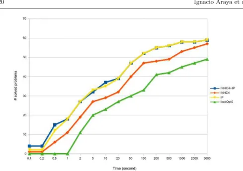
The performance comparison between IbexOpt and IbexOpt0 appears in Table 3 and Fig. 7.
Results
This experiment highlights the significant benefits of our upper bounding, compared to simple probing and inner tests (based on constraint inversion) in every explored outer box. A loss in performance of 31% has been observed in only one instance whereas a speedup of at least a factor 2 has been observed on 33 systems. Furthermore, IbexOpt0 was not able to solve 10 of the 59 selected systems: it reached the timeout in 1 system and raised a memory overflow in 9 systems.
Table 2 Sample of 59 systems selected in the serie 1 of the COCONUT benchmark. name n name n name n
alkyl (rr) 14 ex6 1 4 6 ex9 2 6 16 bearing 14 ex6 2 6 3 ex14 1 2 6 ex2 1 3 13 ex6 2 8 3 ex14 1 6 9 ex2 1 5 10 ex6 2 9 4 ex14 1 7 10 ex2 1 6 10 ex6 2 10 6 ex14 2 1 5 ex2 1 7 20 ex6 2 11 3 ex14 2 3 6 ex2 1 8 24 ex6 2 12 4 ex14 2 4 6 ex2 1 9 10 ex6 2 14 4 ex14 2 6 5 ex2 1 10 20 ex7 2 1 7 ex14 2 7 6 ex3 1 1 8 ex7 2 3 9 haverly 12 ex3 1 3 6 ex7 2 7 (rr) 4 hhfair 28 ex5 2 2 c1 9 ex7 2 8 (rr) 8 himmel11 9 ex5 2 2 c2 9 ex7 2 9 (rr) 10 himmel16 18 ex5 2 2 c3 9 ex7 3 4 12 house 8 ex5 2 4 7 ex7 3 5 13 hydro 30 ex5 3 2 22 ex8 1 8 6 immun (rr) 21 ex5 4 2 8 ex8 5 1 6 launch 38 ex5 4 3 16 ex8 5 2 6 meanvar 7 ex6 1 1 8 ex8 5 3 5 process 10 ex6 1 3 12 ex8 5 6 6
Table 3 Gains obtained by different optimizers X (IbexOpt, InHC4, IP) w.r.t. IbexOpt0. IPdenotes a variant of the optimizer calling only InnerPolytopeUB at each iteration. InHC4 denotes a variant of the optimizer calling only InHC4UB at each iteration. IbexOpt=IP+InHC4 calls InnerPolytopeUB and InHC4UB. The gain is defined by time(IbexOpt0)time(X) . For each line (gain range), the number of problems obtaining that gain is reported for the different opti-mizers. The penultimate line reports the number of systems successfully handled by X but which induce a memory overflow with IbexOpt0.
Gain IbexOpt InHC4 IP <0.69 0 0 0 0.69 – 0.9 1 4 2 0.9 – 1 2 2 2 1 – 1.1 0 11 0 1.1 – 2 14 13 13 2 – 10 19 15 22 10 – 100 11 3 8 >100 3 2 3
Memory overflow (MO) with IbexOpt0 9 7 9 Solved within the timeout 59 57 59
InnerPolytopeseems more useful than InHC4, but endowing a B&B with InnerPolytopeand InHC4 together is more robust and shows a better perfor-mance than using each individually.
Fig. 7 Performance profile. A point on a curve indicates the number of systems solved within the CPU time in abscissa by the corresponding optimizer.
Qualitative study
Several qualitative analyses were conducted on the systems to better under-stand them individually and also to discover some general trends of our upper bounding heuristics.
A first attempt was to determine which of the two inner region extraction heuristics is the most useful in every system. To measure this, we counted the number of times InHC4UB and InnerPolytopeUB improved the upper bound. No general conclusion was drawn because the result does depend on every instance.
We also measured the mean size of outer boxes in which the algorithms succeed in extracting an inner region. Again, no definite trend was observed, but it appears that InHC4UB generally improves the upper bound in boxes that are larger than boxes where InnerPolytopeUB does. This would confirm that an interval Taylor form provides a good approximation of a non-convex function in a small box handled at the bottom of the search tree.
We finally observed a greater variability in runtime when IbexOpt is called with InHC4UB only than with InnerPolytopeUB only. (We tried 10 runs with different seeds for the random number generator.) This is due to the random choices made in the cases 2, 3 and 4 of InHC4UB (in the MonoMaxInnerBox procedure).
6.2 Comparison with other global optimizers
We conclude experiments with a comparison between six competitors belong-ing to the three types of deterministic branch & bounds for constrained global optimization (over the reals) introduced in Section 2:
– Baron [26] and Couenne [3] cannot guarantee their results (see Section 2). In addition, Couenne rewrites the whole system using a DAG-based rep-resentation of the expressions where some common sub-expressions are detected and synthesized. The equations in this DAG are relaxed by two inequalities each, thus making the overall relaxation larger than with the original system.
– IbexOpt and IBBA return a floating-point vector guaranteed to be feasible in a system where the equations are relaxed. Two versions of IbexOpt are tested: the first one (Ibex 1.19) and the latest one (Ibex 2.0).
– Icos and GlobSol rigorously handle the global optimization problem under inequality and equality constraints (see Definition 2).
The rigorous answer of Icos and GlobSol is very interesting, but these interval optimizers are not competitive at all with the others in terms of per-formance. They show a loss of performance of several orders of magnitude compared to Baron or IbexOpt on many difficult instances. Thus, the results do not appear in the performance profile. Tables 2 and 3 in the first paper about IbexOpt [27] show the results obtained by Icos and GlobSol on 32 instances of the above sample.
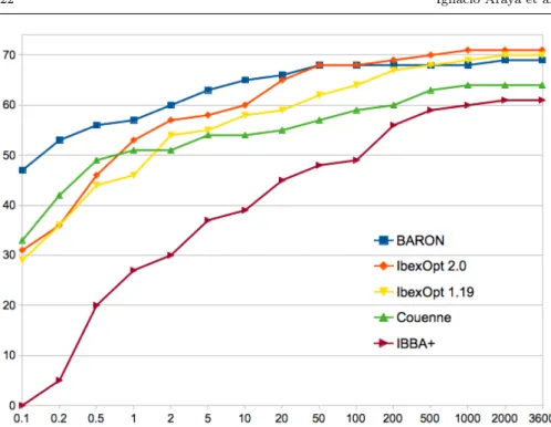
The sample of instances used in the performance profile shown in Fig. 8 comprises the 74 instances tested by Ninin et al. [22] and reused in our AAAI article [27]. This sample allows a comparison with IBBA [22]. All the competitors used the same precision parameters (i.e., 1e-8 for the cost and the relaxation of equations). Most of the competitors were run on the same computer (Intel X86, 3 GHz). Baron was launched on the Neos server (see www.neos-server.org/neos/) also on a X86, thus making the compari-son rather fair. (Other experiments showed that the difference in CPU time between both computers is about 10%.) We can observe that Baron version 12 (June 2013) is generally the most efficient optimizer, but the difference with IbexOpt 2.0 is small, especially after 1 second of CPU time. Note that IbexOpt2.0 solves two more instances than Baron in one hour. In particular, the system ex7 2 3 cannot be solved by Baron within the time limit of 3600 seconds, while this system is solved in less than 100 seconds by IbexOpt 2.0.
IbexOpt compares favorably with Couenne version 0.4 on this sample. It is worthwhile noting Couenne answers that 4 instances have no feasible points (ex3 1 1, ex5 2 4, ex7 3 1, ex14 1 9). This underlines that the lack of rigor is not a theoretical drawback but does lead to failures in practice.
Baronand Couenne seem better than IbexOpt and IBBA on the most simple instances, in part because they can solve some of them during a pre-processing phase. IbexOpt and IBBA are not endowed with these pre-processing tools.
Fig. 8 Performance profile. For a given strategy, a point (t, p) on the corresponding curve indicates that p among the 74 systems are solved in less than t seconds.
However, in 1 or 2 seconds, IbexOpt can solve the same number of systems as Couenne, while IbexOpt 2.0 reaches the performance of Baron in 50 seconds.
IbexOptis (one order of magnitude) more efficient than IBBA and we know that upperbounding with inner regions mainly explains this gain in perfor-mance (see [27]).
7 Conclusion
We have proposed in this paper a new upperbounding policy for systems with inequality constraints (or relaxed equalities). The two proposed heuristics (InnerPolytope and InHC4) first extract an inner (entirely feasible) region and then select a good (or best) point inside the extracted inner region for updating the upper bound with its cost. We have obtained very good results on a representative sample of medium-sized instances proposed in the CO-CONUT benchmark suite. InnerPolytope obtains the best results on the sample, although using both InnerPolytope and InHC4 renders the upper-bounding phase more robust. Overall, endowed with these upperupper-bounding fea-tures, IbexOpt compares favorably with deterministic global optimizers found in the literature, namely Couenne, IBBA, Icos, GlobSol. Baron remains more efficient than IbexOpt, in particular on easy instances or on polynomial ones.
This is not the case for systems with non polynomial operators (division, sine, log, etc).
It is worthwhile noting that our upperbounding does not use any local minimization approach. As shown in Section 5, our heuristics are not costly and are thus used at each node of the interval B&B. In other deterministic optimizers, upperbounding with local minimization is often costly because of the heavy generation of the Lagrangian relaxation. Therefore, these optimiz-ers generally do not call this process at each node of the B&B. We believe that both approaches are complementary, and integrating them together is an interesting line of research.
References
1. Araya, I., Trombettoni, G., Neveu, B.: Exploiting Monotonicity in Interval Constraint Propagation. In: Proc. AAAI, pp. 9–14 (2010)
2. Araya, I., Trombettoni, G., Neveu, B.: A Contractor Based on Convex Interval Taylor. In: CPAIOR, pp. 1–16. LNCS 7298 (2012)
3. Belotti, P.: Couenne, a user’s manual (2013). www.coin-or.org/Couenne/
4. Benhamou, F., Goualard, F.: Universally Quantified Interval Constraints. In: Proc. CP, Constraint Programming, LNCS 1894, pp. 67–82 (2004)
5. Benhamou, F., Goualard, F., Granvilliers, L., Puget, J.F.: Revising Hull and Box Con-sistency. In: Proc. ICLP, pp. 230–244 (1999)
6. Bliek, C.: Computer methods for design automation. Ph.D. thesis, MIT (1992) 7. Chabert, G., Beldiceanu, N.: Sweeping with Continuous Domains. In: Proc. CP, LNCS
6308, pp. 137–151 (2010)
8. Chabert, G., Jaulin, L.: Contractor Programming. Artificial Intelligence 173, 1079–1100 (2009)
9. Collavizza, H., Delobel, F., Rueher, M.: Extending Consistent Domains of Numeric CSP. In: Proc. IJCAI, pp. 406–413 (1999)
10. Goldsztejn, A.: D´efinition et applications des extensions des fonctions r´eelles aux inter-valles g´en´eralis´es: nouvelle formulation de la th´eorie des intervalles modaux et nouveaux r´esultats. Ph.D. thesis, University of Nice Sophia Antipolis (2005)
11. Hansen, E.: Global Optimization using Interval Analysis. Marcel Dekker inc. (1992) 12. Kearfott, R.B.: Rigorous Global Search: Continuous Problems. Kluwer Academic
Pub-lishers (1996)
13. Kreinovich, V., Lakeyev, A., Rohn, J., Kahl, P.: Computational Complexity and Feasi-bility of Data Processing and Interval Computations. Kluwer (1997)
14. Lebbah, Y., Michel, C., Rueher, M., Daney, D., Merlet, J.: Efficient and safe global constraints for handling numerical constraint systems. SIAM Journal on Numerical Analysis 42(5), 2076–2097 (2005)
15. Lin, Y., Stadtherr, M.: LP Strategy for the Interval-Newton Method in Deterministic Global Optimization. Industrial & engineering chemistry research 43, 3741–3749 (2004) 16. McAllester, D., Van Hentenryck, P., Kapur, D.: Three Cuts for Accelerated Interval Propagation. Tech. Rep. AI Memo 1542, Massachusetts Institute of Technology (1995) 17. Messine, F., , Laganouelle, J.L.: Enclosure Methods for Multivariate Differentiable Func-tions and Application to Global Optimization. Journal of Universal Computer Science 4(6), 589–603 (1998)
18. Messine, F.: M´ethodes d’optimisation globale bas´ees sur l’analyse d’intervalle pour la r´esolution des probl`emes avec contraintes. Ph.D. thesis, LIMA-IRIT-ENSEEIHT-INPT, Toulouse (1997)
19. Moore, R., Kearfott, R.B., Cloud, M.: Introduction to Interval Analysis. SIAM (2009) 20. Moore, R.E.: Interval Analysis. Prentice-Hall (1966)
22. Ninin, J., Messine, F., Hansen, P.: A Reliable Affine Relaxation Method for Global Optimization. Tech. Rep. RT-APO-10-05, IRIT (2010)
23. Oettli, W.: On the Solution Set of a Linear System with Inaccurate Coefficients. SIAM J. Numerical Analysis 2(1), 115–118 (1965)
24. Rohn, J.: Inner Solutions of Linear Interval Systems. In: Proc. Interval Mathematics 1985, LNCS 212, pp. 157–158 (1986)
25. Shary, S.: Solving the Linear Interval Tolerance Problem. Mathematics and Computers in Simulation 39, 53–85 (1995)
26. Tawarmalani, M., Sahinidis, N.V.: A Polyhedral Branch-and-Cut Approach to Global Optimization. Mathematical Programming 103(2), 225–249 (2005)
27. Trombettoni, G., Araya, I., Neveu, B., Chabert, G.: Inner Regions and Interval Lin-earizations for Global Optimization. In: AAAI, pp. 99–104 (2011)
28. Trombettoni, G., Chabert, G.: Constructive Interval Disjunction. In: Proc. CP, LNCS 4741, pp. 635–650 (2007)


![Fig. 5 Case 3, procedure MonoMaxInnerBox: The dotted box corresponds to a maximal inner box of [z] w.r.t](https://thumb-eu.123doks.com/thumbv2/123doknet/8031861.269176/13.892.167.554.516.830/fig-case-procedure-monomaxinnerbox-dotted-corresponds-maximal-inner.webp)
![Fig. 6 illustrates the two main cases for the multiplication x 1 .x 2 ∈ [z], depending whether 0 belongs or not to [z].](https://thumb-eu.123doks.com/thumbv2/123doknet/8031861.269176/14.892.116.613.463.612/fig-illustrates-main-cases-multiplication-x-depending-belongs.webp)