To cite this document: Mignot, Rémi and Hélie, Thomas and Matignon, Denis
Digital waveguide simulation of convex acoustic pipes. (2010) In: 13th
International conference on Digital Audio Effects, DAFx’10, 06-10 Sep 2010,
Graz, Austria.
O
pen
A
rchive
T
oulouse
A
rchive
O
uverte (
OATAO
)
OATAO is an open access repository that collects the work of Toulouse researchers and
makes it freely available over the web where possible.
This is an author-deposited version published in:
http://oatao.univ-toulouse.fr/
Eprints ID: 8978
Any correspondence concerning this service should be sent to the repository
administrator:
[email protected]
DIGITAL WAVEGUIDE SIMULATION OF CONVEX ACOUSTIC PIPES
Rémi Mignot
∗ †, Thomas Hélie,
IRCAM & CNRS, UMR 9912
1, pl. Igor Stravinsky,
75004 Paris, France
{mignot,helie} @ ircam.fr
Denis Matignon
ISAE, Applied Mathematics Training Unit,
10, av. E. Belin, B.P. 54032.
F-31055 Toulouse cedex4, France
denis.matignon @ isae.fr
ABSTRACT
This work deals with the physical modelling of acoustic pipes for real-time simulation, using the “Digital Waveguide Network” approach and the horn equation. With this approach, a piece of pipe is represented by a two-port system with a loop which in-volves two delays for wave propagation, and some subsystems without internal delay. A well-known form of this system is the “Kelly-Lochbaum” framework. It allows the reduction of the com-putation complexity and it gives a physically meaningful interpre-tation of the involving subsystems.
In this paper, we focus this work on the simulation of pipes with a convex profile, for which a curvature coefficient is constant and negative. In the literature, it has been shown that such pipes have trapped modes. With the formalism of automatic control, adapted for “Waveguides”, we meet some substates of the system which do not take effect on the outputs.
But, using the “Kelly-Lochbaum” framework with the horn equation, two problems occur: first, even if the outputs are bound, some substates have their values which diverge; second, there is an infinite number of such substates. The system is then unstable and cannot be simulated as such.
The solution of this problem is obtained with two steps. First, we show that there is a simple standard form compatible with the “Waveguide” approach, for which there is an infinite number of solutions which preserve the input/output relations. Second, we look for one solution which guarantees the stability of the system and which makes easier the approximation in order to get a low-cost simulation.
1. INTRODUCTION
In [1] and [2], the physical modelling of acoustic wave propagation in convex pipes has been studied, and these studies have shown the presence of trapped modes. Similarly to the model of cone connec-tions with a negative change of slope (cf. eg. [3]), some problems of stability occur. Since these instabilities have no influence in a global point of view, for the simulation some solutions have con-sisted in considering the system in a global point of view, using for example a modal approach or a digital convolution with finite impulse response filters.
But, for digital simulations with low-cost computations, the modal approaches need the truncation of modes, which involve some problems of realism. And because of some long memory ef-fects (of the diffusive type for visco-thermal losses for example)
∗Rémi Mignot is Ph.D. student at Télécom ParisTech/TSI.
†This work is supported by the CONSONNES project,
ANR-05-BLAN-0097-01.
the convolution methods are not adapted because the impulse re-sponses decrease very slowly.
In [4], flared pipes have been modelled with the Digital Wave-guide Network approach (cf. eg. [5]) using the horn equation of Webster (cf. [6]) and taking into account the visco-thermal losses (cf. [7, 8]). The simulation framework of Kelly-Lochbaum has been obtained (cf. eg. [9]). This system involves some delays for wave propagation through pieces of pipe, and some recursive filters for reflections and transmissions at junctions of pieces of pipe. This model leads to real-time simulations.
Nevertheless, the application of the latter model to convex pipes produces some stability problems. The aim of this work is to get a stable digital realization for convex pipes, similar to this one of [4].
This paper is organized as follow. Section 2 presents the acous-tic model we use, the Webster-Lokshin model, and 2 equivalent systems for the simulation. In sec. 3, we study in the Laplace domain the singularities of the transfer functions involved in this model, and we explain the reason of their presence in the case of convex pipes. In sec. 4, we propose a “generalized” framework for simulation, which allows the description of the acoustic model with 2 degrees of freedom, which are 2 transfer functions of the system. In sec. 5, we choose 2 transfer functions which allow a stable digital simulation for convex pipes. This solution is com-patible with the Waveguide approach and it is similar to [4]. The last section concludes this paper and deals with perspectives.
2. ACOUSTIC MODEL AND SYSTEMS 2.1. The Webster-Lokshin model
The Webster-Lokshin model is a mono-dimensional model which characterizes the linear propagation of acoustic waves inside ax-isymmetric pipes, with the weak hypothesis of quasi-sphericity of isobares near the wall (cf. [8]), and taking into account the visco-thermal losses at the wall with the hypothesis of large tubes (cf. [7, 10]). The acoustic pressureP and the volume flow U are gov-erned by the following equations, given in the Laplace domain:
s2 c2+2ε(ℓ) s32 c32 +Υ(ℓ) − ∂ 2 ∂ℓ2 !n r(ℓ)P (ℓ, s)o= 0, (1) ρ sU (ℓ, s) S(ℓ) + ∂ ∂ℓP (ℓ, s) = 0, (2) wheres ∈ C is the Laplace variable (ℑm(s) = ω is the pulsation), ℓ is the curvilinear abscissa at the wall, r(ℓ) is the radius of the pipe,S(ℓ) = πr(ℓ)2is the section area,ε(ℓ) = κ
0p1−r′(ℓ)2/r(ℓ)
represents the curvature of the pipe. Equation (1) is the Webster-Lokshin equation, and (2) is the Euler equation satisfied outside the boundary layer.
2.2. Two equivalent systems
We define a piece of pipe by a tube with a finite lengthL and with constant coefficients of losses and curvature (ε and Υ). We will build two systems which represent the acoustic effects of a piece of pipe on the travelling waves given by:
φ±= r 2 “
P ± ZU”, where Z(ℓ) = ρc
S(ℓ). (3) In [4], the effects of a piece of pipe on the variablesφ±are
rep-resented by input/ouput systems for the Webster-Lokshin model. Two equivalent forms (in an input/output point of view) are given. A first form, so-called “global”, is given in Fig. 1-(a). Its 4 transfer functions represent global effects of the piece of pipe on the wavesφ±:Rl
gandRgrare the left and right reflections
respec-tively, andTgis the global transmission through the piece of pipe.
“global” means that all internal acoustic effects are mixed, for ex-ample the forwards and backwards of wave propagation are taken into account.
A second form, so-called “decomposed”, is given by Fig. 1-(b). This form is interesting because it isolates the internal acoustic ef-fects inside some transfer functions. For example,Rlerepresents
the reflection ofφ+0 at the left interface, andT represents the prop-agation through the piece of pipe. Here the successive forwards and backwards are represented by the internal loop. This form al-lows the recovery of the Kelly-Lochbaum framework which is well adapted for digital real-time simulation (cf. eg. [9]).
(a) (b) Rl g Tg Tg Rr g φ+ 0 φ + 0 φ− 0 φ−L φ−0 φ − L φ+ L φ+L Qp Q Qr Ql Rle R li 1+Rle 1+Rli Rre Rri 1+Rre 1+Rri T T
Figure 1: Two-port Q (global form) and its decomposed form. Let’s defineΓ(iω) = ik(ω), where k(ω) is the standard com-plex wavenumber. In the Laplace domain, the functionΓ is given by Γ(s) =r“s c ”2 + 2ε“ s c ”3 2 + Υ. (4)
The analytical solving of (1) and (2) gives the functions of Q Tg = {ATcosh(ΓL) + BTsinh(ΓL) / Γ}−1, (5) Rl g = {ARcosh(ΓL) + BRlsinh(ΓL) / Γ} Tg, (6) Rr g = {ARcosh(ΓL) + BRrsinh(ΓL) / Γ} T g, (7)
whereAT,AR,BT,BRlandBRrare some known functions ofs
andΓ(s)2. Withζ = r′/r, the functions of the decomposed form
are given in [4]: T (s) = e−Γ(s)L, (8) Rle(s) = s c−Γ(s)−ζl s c+Γ(s)+ζl , Rli(s) = − s c−Γ(s)+ζl s c+Γ(s)+ζl , (9) Rre(s) = s c−Γ(s)+ζr s c+Γ(s)−ζr , Rri(s) = − s c−Γ(s)−ζr s c+Γ(s)−ζr . (10)
Withτ := L/c, note that we can write Tg(iω) = Dg(iω) e−iωτ
andT (iω) = D(iω) e−iωτ, whereDg and D are two transfer
functions associated to causal systems (forΥ ≥ 0). Consequently, the impulse responses ofTg andT are these ones of Dg andD
delayed byτ which corresponds to the time of propagation inside the piece of pipe.
In the case of pipes with negative curvatures (Υ < 0) these two forms present a paradox: whereas some numerical calculus reveal that the global form of Fig. 1-(a) is stable, the transfer func-tions of the decomposed form of Fig. 1-(b) have some singularities in the Laplace domain which produces some instabilities. The aim of the following section is the understanding of the reason of this problem.
3. ANALYSIS OF SINGULARITIES 3.1. Complex analysis ofΓ
The functionΓ(s) (associated to the wavenumber k(ω), cf. (4)) is defined as a square root of a complex number which depends itself on a square root ofs. But there is an infinite number of continuations of the positive square root defined on R+ for the complex plan, and we must choose one of them in order to define in C the transfer functions of the system.
In [11, 12], the functionΓ is defined by the choice of curves (called cut) which link some branching points to the infinity. These cuts are continuous sets of singularities, which produce some dis-continuities ofΓ. And the branching points snare the solutions of
Γ(s)2= 0, and s
0= 0 (for√s).
Υ = 0: For cylindrical and conical pipes, the unique branching point iss0= 0.
Υ > 0: For flared pipes, Γ has 3 branching points: s0= 0, s1and
s2= s1, withℜe(s1) ≤0.
Υ < 0: For convex pipes, Γ has 2 branching points: s0 = 0, and
s1∈ R+.
Whereas these branching points are fixed (they depend onc, ε and Υ), the cuts have to be chosen.
ForΥ ≥ 0, since no branching point is in the right-half Laplace plane (denoted C+0 := {s ∈ C/ ℜe(s) > 0}), it is possible to define an analytical continuation over C+0 in order to respect the stability of the transfer functions. For example, the case of horizontal cuts is presented in Fig. 2.
However, forΥ < 0, one branching points, s1, is in C+0, and
so it is not possible to define a analytical continuation over C+0 since at least one part of the cut is in C+0. Figure 2 presents the case of 2 overlapped cuts on R−:]−∞, 0] and ]−∞, s1].
−4000 −2000 0 2000 −2000 −1000 0 1000 2000 −4000 −2000 0 2000 −2000 −1000 0 1000 2000 −4000 −2000 0 2000 −2000 −1000 0 1000 2000 s1 s1 s2 s0 s0 s0 ℜe(s) ℜe(s) ℜe(s) ℑm(s) ℑm(s) ℑm(s) −π − π2 0 + π2 +π Υ > 0 Υ = 0 Υ < 0
Figure 2: Phase ofΓ(s) in the complex plan, branching points and horizontal cuts.
3.2. Poles and physical interpretation
Whereas the transfer functions of the decomposed form (cf. (8-10)) have the same type of singularities thanΓ (of the cut type), the 3 global transfer functions (cf. (5-7)) only depends onΓ(s)2
and notΓ(s) (they are invariant with the transformation Γ 7→ −Γ). Thus these 3 transfer functions have only one cut which comes from√s, and some other singularities of the pole type which are associated to the resonance modes of the piece of pipe.
This last remark implies that only the transfer functions of the decomposed form depend on the choice ofΓ. The input/output relations do not depend on the choice of the cuts which start from s1ands2(because of the curvature) but they only depend on the
cut which starts froms0= 0 (because of the visco-thermal losses).
For this branching point, we will choose R−for some reasons of stability and hermitian symmetry.
In [13],Γ is given by √. defined by
√. : s = ρ exp(iθ) 7→√s =√ρ exp(iθ/2),
(11) with(ρ, θ) ∈ R+∗×] − π, π]. With this choice of Γ, the set of the cuts is R−∪ C with C := {s ∈ C/ Γ(s)2 ∈ R−}. With this
definition,Γ has the following property:
∀s ∈ C \ C, ℜe(Γ(s)) > 0. (12) Consequently, whenL increases,
∀s ∈ C \ C, T (s) = e−Γ(s)L→ 0, when L → ∞. (13) Thus, in the decomposed form of Fig. 1-(b), T (s) behaves as a “circuit breaker” at the limit. And so, we prove the following result
∀s ∈ C \ C, lim
L→∞R l
g(s) = Rle(s). (14)
The functionRleis then interpretated as the global reflection
of a semi-infinite pipe (anechoic). A similar reasoning has been done in [3] for cones.
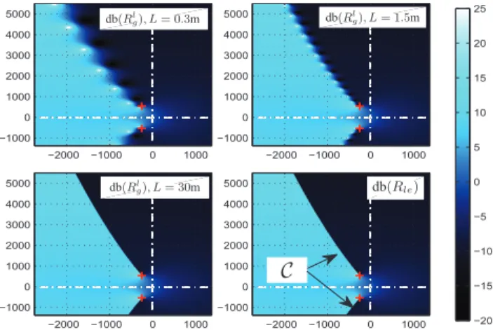
We observe the convergence of poles and zeros ofRl gtowards
the cutC of RlewhenL increases. Thus, the cut can be
interpre-tated as a densification of intertwined poles and zeros. Figure 3 illustrates this convergence withΥ > 0.
−2000 −1000 0 1000 −1000 0 1000 2000 3000 4000 5000 −2000 −1000 0 1000 −1000 0 1000 2000 3000 4000 5000 −2000 −1000 0 1000 −1000 0 1000 2000 3000 4000 5000 −2000 −1000 0 1000 −1000 0 1000 2000 3000 4000 5000 −20 −15 −10 −5 0 5 10 15 20 25 db(Rl g), L = 0.3m db(R l g), L = 1.5m db(Rl g), L = 30m db(Rle)
C
Figure 3: Convergence of poles and zeros ofRl
g whenL → ∞
(withΥ > 0). Poles, zeros and branching points are represented by white points, black points and red crosses respectively.
3.3. Interpretation forΥ < 0
For negative curvatures, because of the part of the cut on[0, s1] ⊂
R+, the associated functions have an infinite number of singulari-ties which produce instabilisingulari-ties. But some numerical observations show that the global transfer functions of the piece of pipe, which have not this cut, are stable as expected.
A pipe with constant and negative curvatureΥ = r′′/r has a
sinusoidal profiler(ℓ) which changes sign every Lcrit:= π
p |Υ|. But we observe that whenL increases, a pole pkofRlg becomes
unstable as soon as the lengthL of the piece of pipe exceeds kLcrit
(withk ∈ N∗). Figure 4 illustrates this.
−1000 −500 0 500 1000 −500 0 500 1000 1500 2000 2500 −1000 −500 0 500 1000 −500 0 500 1000 1500 2000 2500 −1000 −500 0 500 1000 −500 0 500 1000 1500 2000 2500 −1000 −500 0 500 1000 −500 0 500 1000 1500 2000 2500 −20 −15 −10 −5 0 5 10 15 20 25 p1 p1 p1 p1 p2 p2 p2 p2 db(Rl g),LcritL = 0.9 db(R l g),LcritL = 1.1 db(Rl g),LcritL = 1.9 db(R l g),LcritL = 2.1
Figure 4: Pole transition from C−0 to R+, withΥ < 0. In this case, whenL → ∞ there is a densification of an in-finite number of unstable poles on[0, s1]. Thus, for L < Lcrit
the global transfer functions of the piece of pipe are stable, but the transfer functions of the decomposed form, which are associ-ated to a semi-infinite pipe, have an infinite number of unstable singularities. This phenomenum comes from the decomposition of Fig. 1-(b) which is well adapted to digital waveguide simula-tions with positive curvatures. For negative curvatures, we have to search another decomposition which is adapted to waveguides and which is stable forΥ < 0.
4. GENERALIZED FRAMEWORK 4.1. Global form and decomposed form
We have seen that the piece of pipe can be modelled by 2 systems (cf. Fig. 1). The first is given by the two-port Q and its 4 global functions; and the second is given by a decomposed form with 10 transfer functions.
• Global form: No matter the sign of the curvature coeffi-cientΥ, the transfer functions Rl
g,Rrg, andTg are stable.
Moreover, we have seen that they have only one cut on R− because of the visco-thermal losses. Their simulation with a modal approach, could allow a stable realization of the piece of pipe. But the low-cost computation need the trun-cation of modes, which involves some problems of realism. • Decomposed form: This form is adapted to the waveguide modelling, but it implies some problems of stability. With Υ < 0 an unstable part of the cut appears on R+.
In the next section, we see that there is an infinite number of forms of a piece of pipe, and then we get a parametrization in order to find a stable realization which respects the waveguide forma-lism.
4.2. Standard form of a piece of pipe
In a first time, we represent the 2 forms of Fig. 1 with a common framework: the framework of Fig. 5 is equivalent to the 2 forms (global or decomposed) if the following equations hold:
• Global form: Hl= Rlg, Fl= Dg, Gl= 0, Hr= Rrg, Fr = Dg, Gr= 0. • Decomposed form: Hl= Rle, Fl= D(1 + Rri)(1 + Rle), Hr= Rre, Fr= D(1 + Rli)(1 + Rre), Gl=RliD(1+R1+Rliri), Gr=Rri1+RD(1+Rri li).
whereD and Dgcorrespond to the transmissionsT and Tg
with-out delay: T (s) = D(s) e−τ s andT
g(s) = Dg(s) e−τ s. The
other functions of the decomposed form are given by (8-10).
Gl Gr Hl Hr Fl Fr e−τ s e−τ s φ+ L φ− 0 φ − L φ+0
Figure 5: Standard form of a piece of pipe
4.3. Parametrization
In a general case, the standard form (Fig. 5) allows the representa-tion of a piece of pipe if the following algebraic equarepresenta-tions hold
Rl g = Hl+ ` FlGre−2τ s ´ /`1 − GlGr e−2τ s ´ , (15) Rr g = Hr+ ` FrGle−2τ s ´ /`1 − GlGr e−2τ s ´ , (16) Dg = Fl/ ` 1 − GlGr e−2τ s ´ , (17) = Fr/`1 − GlGr e−2τ s´. (18)
We observe that this system of equations has 2 degrees of free-dom. ChoosingGlandGras degrees of freedom, the solving of
the system (15-18) gives
Hl = Rlg− DgGre−2τ s, (19) Hr = Rrg− DgGle−2τ s, (20) Fl = Dg ` 1 − GlGre−2τ s ´ , (21) Fr = Dg ` 1 − GrGre−2τ s ´ . (22)
Consequently, it is possible to choose arbitrarily the functions GlandGrand to preserve the original input/ouput relations of the
system. And so we have a parametrization of the system with 2 functions. For example the global form corresponds to the choice:
Gl= 0, Gr= 0.
In the case of the decomposed form, the 6 transfer functions have no internal delay, the modes of the piece of pipe are simulated by the loop. For the global form,Gl= Gr = 0, the loop is open,
and the modes are simulated by the delays in the denominator of the 4 other functions.
Remarks: For all causal and stableGlandGr, the 4 functionsHl,
Hr,FlandFrdefined by (15-18) are causal and stable. Moreover,
the choiceGlandGrsuch as|Gl(s)| < 1 and |Gr(s)| < 1, ∀s ∈
C+0, allows the guarantee of the stability of the internal loop of the system.
Now we have to findGlandGrwhich allow to guarantee the
stability and the passivity of the system, and to preserve the wave-guide formalism.
5. STABLE REALIZATION OF CONVEX PIPE 5.1. Stabilization of convex pipes
With the waveguide approach, the “ideal” choice is this one of the decomposed form. With
R∗li:= Rli(1 + Rri) 1 + Rli D et R∗ri:= Rri(1 + Rli) 1 + Rri D, (23) this “ideal” choice is given byGl = R∗lietGr = R∗ri. But these
functions depend onΓ and they have some unstable singularities on[0, s1] with Υ < 0. We should do another choice.
5.1.1. What can be a “good choice”?
Qualitatively, in order to understand what is a “good choice” ofGl
andGrwe can examine for example the expression of the function
Flgiven by (21): Fl(s) = Dg(s) ` 1 − Gl(s)Gr(s) e−2τ s ´ .
The functionDg has a cut on R−because of losses, and an
infinite number of pairs of complex conjugate poles in C−0. Every pair corresponds to a mode of the piece of pipe. These poles are the zeros of the denominator ofDgwhich is:1 − R∗liR∗rie−2τ s. The
choiceGl= R∗liandGr= R∗ri, allows the exact compensation of
the poles ofDg. With this choice,Flhas no pole as singularity,
but only the cutC of Γ.
The idea we propose and test here, is to compensate the high frequency poles (there is a infinite number) by the internal loop of the framework with a choice such asGl(iω) ≈ R∗li(iω) and
Gl(iω) ≈ R∗ri(iω) when |ω| is high, but with Gland Gr
holo-morphic in C+0. Finally, the staying poles in low frequencies are simulated as such in the 4 transfer functionsHl,Hr,FlandFr
given by (19-22).
5.1.2. How to find a “good choice”?
For simplification, we artificially modify the functionsR∗ liandR∗ri
with a mappings 7→ γ(s) of the complex plan:
Gl(s) := R∗li(γ(s)), and Gr(s) := R∗ri(γ(s)). (24)
Now the choice ofGlandGris done by the choice of this
“map-ping”. To guarantee a good behavior in high frequency (Gl(iω) ≈
R∗
li(iω) and Gl(iω) ≈ R∗ri(iω)), we choose γ such as:
∀s ∈ C+0 with|s| high: γ(s) ≈ s. (25)
Remark: The expression “|s| high” is voluntarily imprecise. In practice, we want thatγ(iω) goes quickly towards iω when |ω| increases.
5.1.3. Properties of a “good mapping”
Not onlyγ have to verify (25), but it is also interesting to control the singularities ofGlandGrwith the choice ofγ. In a first time
the chosen mapping has to guarantee the stability and the passivity ofGlandGr, and if possible it has to reduce the set of their
sin-gularities. To guarantee the good definition of these functions, we give some constraints:
P1: γ is hermitian (for real signals), P2: γ is analytical in C+0, P3: ] − ∞, s1] ∩ γ`C+0 ´ = {∅}, P4: ∀s ∈ C+0, |R∗ li(γ(s))| < 1 et |R∗ri(γ(s))| < 1.
With these properties, the choice Gl(s) := R∗li(γ(s)) and
Gr(s) := R∗ri(γ(s)) defines some hermitian functions (P1),
holo-morphic in C+0 (P2, P3 and becauseR∗
liandR∗riare holomorphic
on C\ ]−∞, s1]) and P4 guarantees the stability of the loop.
Note that the set of the cuts ofGl and Gr becomesC† :=
{s ∈ C/ γ(s) ∈] − ∞, s1]} (with C† ⊂ C−0 thanks to P3). Thus
the mappingγ allows the “rejection” of the unstable part of the cut ofΓ ([0, s1] ⊂ R+) in C−0, this stabilize the transfer functions.
5.2. Stable digital realization
Now we give some results of stable realizations of a piece of pipe with a negative curvature. We use the previous idea, but with some empirical considerations.
The procedure is summarized by the following steps: • We choose the parameter functions GlandGrusing a
map-pingγ.
• We deduce Hl,Hr,FlandFr.
• We approximate the 6 transfer functions using standard re-cursive filters.
5.2.1. Definition of the mapping
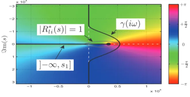
In practice, instead of looking for a well definedγ in C, we limit the search in iR (Fourier domain). Thus, we look for a contour given byγ(iR).
In high frequencies, the contour must get closer to the imagi-nary axis (cf. (25)), and so we choose it such asγ(iω) = iω with |ω| > ω0, whereω0is a pulsation we can name junction pulsation.
In lower frequencies, this contour has not only to get around the part[0, s1] of the cut (to guarantee P3), but also to get around
the set ofs ∈ C such as |R∗
li(s)| > 1 and |R∗ri(s)| > 1 (P4).
Moreover, this contour must verify a constraint ofC∞
-regula-rity oniR (necessary condition for P2). Thus, the “junction” in ω = ±ω0 between low and high frequencies must has the
conti-nuity of all its derivatives.
In order to simulate only the 2 first modes of the piece of pipe, the junction pulsationω0is chosen equal toℑm(p2) where p2 is
the pole associated to the second mode of the piece of pipe. Figure 6 illustrates the contourγ(iω) which gets around the cut, and the contour line of 1.
5.2.2. Approximation and results
Previously, we have chosen a mappingγ which defines the param-eter functionsGlandGr. Then, we deduceHl,Hr,FlandFr
−1 −0.5 0 0.5 1 x 10⁴ −3 −2 −1 0 1 2 3 x 10⁴ −π − π2 0 + π2 +π ℑ m (s ) |R ∗ li(s)| = 1 γ(iω) ]−∞, s1] Figure 6: Phase ofR∗
liand contourγ(iω).
which preserve the input/output relations of the system using (19-22). For a given piece of pipe this choice allows the definition of a system composed by stable transfer functions, and which contains a stabilized delay loop (|Gl| < 1 and |Gr| < 1 in C+0), cf. Fig. 5.
For the digital realization of the system, first the transfer func-tionsGland Gr are approximated by standard recursive filters.
This type of approximations is presented in [11, 12]; here it need a placement of some poles on R−.
ForHl, Hr,Fl andFr, the same type of approximation is
realized. Here, with|ω| > ω0,Gl(iω) = R∗li(iω) and Gr(iω) =
R∗
ri(iω), in consequence the modes with frequencies higher than
ω0 are simulated by the internal loop of the system. Then, there
are two staying modes which are simulated by 2 pairs of complex conjugate poles.
For evaluation, we have built the realization of a convex piece of pipe with the following parameters:r0 = 7 cm, rL= 10 cm,
Υ = −100 m−2,L = 15 cm, et ε = 0.0033 m−1
2. The junction
pulsation is fitted according to the second mode of the piece of pipe which corresponds to a pair of poles atω0≈ 17 103rad.s−1
(F0 = ω0/(2π) ≈ 2700 Hz). Every transfer function GlorGr
is simulated by 6 stable poles (on R−) and every function among the 4 other by 6 stable real poles and 2 pairs of complex conjugate poles. The delays of the framework of Fig. 5 are simulated by low-cost digital delays (circular buffers).
Figure 7 illustrates the frequency response ofHland its
ap-proximation. We observe 2 lobes which correspond to the 2 first resonances of the piece of pipe which are not simulated by the internal loop. 0 1000 2000 3000 4000 5000 6000 7000 8000 9000 10000 −30 −25 −20 −15 −10 −5 0 Hl(iω) f Hl(iω) d b (H (iω ))
Figure 7:Hland its approximation fHl.
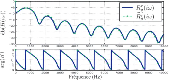
The result of the simulation is illustrated in Fig. 8 by the fre-quency response of the global transfer functionRr
gand of its
sim-ulated version fRr
g. Note that the maximal error is almost 1.9 dB,
0 1000 2000 3000 4000 5000 6000 7000 8000 9000 10000 −35 −30 −25 −20 −15 −10 −5 0 0 1000 2000 3000 4000 5000 6000 7000 8000 9000 10000 −π −π 2 0 π π 2 Rr g(iω) f Rr g(iω) Fréquence (Hz) d b (H (iω )) a rg (H ) Figure 8:Rr
gand its simulated version fRrg.
6. CONCLUSION
In this paper, we have seen in the case of convex pipes that the use of the simulation framework of [4] produces some problems of stability, because of the presence of unstable singularities which are not of the pole type, but of the cut type. After an explanation of the problem, we have proposed a “generalized” framework which parameterizes the system with 2 degrees of freedom which are 2 transfer functions. Then in part 5 we have done a choice which stabilizes the system and preserve the approach of [4]. This choice allows the “rejection” of the unstable singularities to the left-half Laplace plane, this stabilizes them. Finally, the digital simulation of a piece of pipe has been realized with 2 delays and 6 standard recursive filters.
The approach we use here is a little bit empirical and it needs a theoretical study more rigorous. For example, the choice of the mappingγ presented here, only guarantees that the singularities leave to C−0, it seems interesting to guarantee that they go to R− only.
Moreover, only the stability of one piece of pipe is done. For the simulation of a whole virtual pipe, which is the concatenation of several pieces of pipe, it is necessary to study the stability of the whole system.
7. REFERENCES
[1] D. P. Berners, Acoustics and signal processing techniques for physical modeling of brass instruments. PhD thesis, Stand-ford University, 1999.
[2] V. Pagneux, Propagation acoustique dans les guides à sec-tion variable et effet d’écoulement. PhD thesis, Université du Maine, 1996.
[3] J. Gilbert, J. Kergomard, and J.-D. Polack, “On the reflection functions associated with discontinuities in conical bores,” J. Acoust. Soc. Am., vol. 87, no. 4, pp. 1773–1780, 1990. [4] T. Hélie, R. Mignot, and D. Matignon, “Waveguide
mode-ling of lossy flared acoustic pipes: Derivation of a Kelly-Lochbaum structure for real-time simulations,” in IEEE WASPAA, (Mohonk, USA), pp. 267–270, 2007.
[5] J. O. Smith, “Music applications of digital waveguides,” Tech. Rep. STAN-M-39, Center for Computer Research in Music and Acoustics (CCRMA), Department of Music, Stan-ford University, 1987.
[6] A. Webster, “Acoustic impedance and the theory of horns
and of the phonograph,” Proc. Nat. Acad. Sci. U.S, vol. 5, pp. 275–282, 1919.
[7] J.-D. Polack, “Time domain solution of Kirchhoff’s equation for sound propagation in viscothermal gases: a diffusion pro-cess,” J. Acoustique, vol. 4, pp. 47–67, February 1991. [8] T. Hélie, “Unidimensional models of acoustic propagation
in axisymmetric waveguides,” J. Acoust. Soc. Am., vol. 114, pp. 2633–2647, 2003.
[9] J. D. Markel and A. H. Gray, “On autocorrelation equations as applied to speech analysis,” IEEE Trans. Audio and Elec-troac., vol. 21, April 1973.
[10] A. A. Lokshin and V. E. Rok, “Fundamental solutions of the wave equation with retarded time,” Dokl. Akad. Nauk SSSR, vol. 239, 1978.
[11] G. Montseny, “Diffusive representation of pseudo-dif-ferential time-operators,” ESAIM: Proc, vol. 5, pp. 159–175, 1998.
[12] T. Hélie, D. Matignon, and R. Mignot, “Criterion de-sign for optimizing low-cost approximations of infinite-dimensional systems: Towards efficient real-time simula-tion,” in IFAC Workshop on Control Applications of Opti-misation (CAO’06), (Cachan, France), 2006. 6 pages. [13] R. Mignot, T. Hélie, and D. Matignon, “On the appearance
of branch cuts for fractional systems as a mathematical lim-iting process based on physical grounds,” in IFAC Fractional Differentiation and its Applications, (Ankara, Turkey), 2008. 6 pages.
[14] V. Pagneux, N. Amir, and J. Kergomard, “A study of wave propagation in varying crosssection waveguides by modal decomposition. Part I: Theory and validation,” J. Acoust. Soc. Am., vol. 100, no. 4, pp. 2034–2048, 1996.