State-space representation for digital waveguide networks of lossy flared acoustic pipes

To cite this document: Mignot, Rémi and Hélie, Thomas and Matignon, Denis

State-space representation for digital waveguide networks of lossy flared acoustic

pipes. (2009) In: 12th International conference on Digital Audio Effects,

DAFx’09, 01-04 Sep 2009, Como, Italy.

O

pen

A

rchive

T

oulouse

A

rchive

O

uverte (

OATAO

)

OATAO is an open access repository that collects the work of Toulouse researchers and

makes it freely available over the web where possible.

This is an author-deposited version published in:

http://oatao.univ-toulouse.fr/

Eprints ID: 8977

Any correspondence concerning this service should be sent to the repository

administrator:

[email protected]

STATE-SPACE REPRESENTATIONS FOR DIGITAL WAVEGUIDE NETWORKS OF LOSSY

FLARED ACOUSTIC PIPES

Rémi Mignot

, Thomas Hélie,

IRCAM & CNRS, UMR 9912

1, pl. Igor Stravinsky,

75004 Paris, France

{mignot,helie} @ ircam.fr

Denis Matignon

ISAE, Applied Mathematics Training Unit,

10, av. E. Belin, B.P. 54032.

F-31055 Toulouse cedex4, France

denis.matignon @ isae.fr

ABSTRACT

This paper deals with digital waveguide modeling of wind instru-ments. It presents the application of state-space representations to the acoustic model of Webster-Lokshin. This acoustic model describes the propagation of longitudinal waves in axisymmetric acoustic pipes with a varying cross-section, visco-thermal losses at the walls, and without assuming planar or spherical waves. More-over, three types of discontinuities of the shape can be taken into account (radius, slope and curvature), which can lead to a good fit of the original shape of pipe. The purpose of this work is to build low-cost digital simulations in the time domain, based on the Webster-Lokshin model. First, decomposing a resonator into independent elementary parts and isolating delay operators lead to a network of input/output systems and delays, of

Kelly-Lochbaum network type. Second, for a systematic assembling of

elements, their state-space representations are derived in discrete time. Then, standard tools of automatic control are used to reduce the complexity of digital simulations in time domain. In order to validate the method, simulations are presented and compared with measurements.

1. INTRODUCTION

Studying physical modeling for sound synthesis allows to simu-late the behavior of musical instruments. Consequently it naturely leads to realistic sounds, especially during attacks and note transi-tions, compared to signal processing approaches. However, digital simulations in time domain require intensive computations from signal processors, and simplifications of the physical model have to be considered to make real-time simulations possible. More-over, because of interactions between elements of an instrument, building a modular synthetizer proves difficult.

With the approach of digital waveguides (cf. eg. [1]), some works have considered 1D acoustic model of axisymmetric pipes based on the Webster horn equation (cf. [2]). Approximating a varying cross-section pipe by some cylinders or cones leads to the Kelly-Lochbaum scattering network (cf. eg. [3, 4]), which allows a low-cost digital simulation in time domain. These mod-els assume planar and spherical waves respectively. For a more realistic behavior of the virtual instrument, in [5] and [6] visco-thermal losses have been taken into account. This model of losses (cf. [7]) involves fractional derivatives, and is more accurate than more standard dampings based on integer order derivatives. In [8],

∗_{Rémi Mignot is Ph.D. student at Télécom ParisTech/TSI}

†_{This work is supported by the CONSONNES project,} ANR-05-BLAN-0097-01

the Kelly-Lochbaum network has been derived for pipes with

con-tinuity of radius and slope (C1-regularity of the shape), using the

Webster-Lokshin acoustic model of lossy flared pipes which does

not assume planar or spherical waves (cf. [9]).

After modeling each piece of pipe separately, it is necessary to put them together in order to build the whole resonator. In [10] and [11], the following modular method is proposed: deriving

state-space representations of every pieces of pipe in discrete time

do-main, interconnection laws allow to calculate the state-space rep-resentation of the whole resonator. This formalism facilitates the modularity of the building of a virtual trombone.

In a recent work [12], a framework (based on the

Webster-Lokshin equation) has been derived and allows to recover all

mod-els mentioned above ([3, 5, 4, 6, 8]). Moreover, it allows to ob-tain a good level of accuracy with a small number of pipes. The novelty of the present work is the use of the formalism of [11], starting from the unifying model of [12]. Thanks to the modular-ity of the method, virtual wind instruments can be built connecting additional models such as: mouth-piece, radiation, tone-hole, lips and reed (which are not studied in this paper). For example, Fig. 1 presents the network of a possible virtual resonator built by con-necting such acoustic elements.

p+ e p− e ps,1 ps,2

Figure 1: Example of an acoustic network modeling a resonator with a mouth-piece, a horn and a tone-hole.

This document is organized as follows. In section 3, a pipe with varying cross-section is separated into some pieces of pipe. Using the Webster-Lokshin model, each piece of pipe is modeled by an input/output network of the Kelly-Lochbaum type. In section 4, a state-space representation is derived for the network of section 2, in continuous time and in discrete time. Section 5 presents stan-dard tools of automatic control which allow to optimize numerical realizations in order to obtain low-cost digital simulations in the time domain. Section 6 presents the digital simulations of virtual trombones and a comparison between computed impedances and the measured impedance of a real trombone. The last section con-cludes this paper and deals with perspectives.

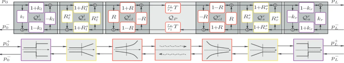
p+ 0 p+ 0 p− 0 p− 0 p− L p− L p+ L p+ L QP Ql a R Qls Rls Qcll Qrcl Qsr Qar s l Rsr _Rs r 1+Rs l 1+Rs l 1+Rs r 1+Rs r kl _k r 1+kl 1+kr −kl −kr 1−kl 1−kr R _−R −R _R 1+R 1+R 1−R 1−R rl rrT rr rlT

Figure 2: Separation of the effects of pipe geometry.

2. MODELING A PIECE OF PIPE 2.1. Webster-Lokshin model and traveling waves

The Webster-Lokshin model is a mono-dimensional model which characterizes linear waves propagation in axisymmetric pipes, as-suming the quasi-sphericity of isobars near the inner wall (cf. [9, 13]), and taking into account visco-thermal losses (cf. [7]) at the

wall. The acoustic pressureP and the particle flow U are governed

by the following equations, given in the Laplace domain: " „ s c0 «2 +2ε(ℓ) „ s c0 «3 2 +Υ(ℓ) ! −∂2ℓ # r(ℓ)P (ℓ, s) = 0, (1) ρ0sU (ℓ, s) S(ℓ) + ∂ℓp(ℓ, s) = 0, (2)

wheres ∈ C is the Laplace variable, ℓ is the space variable

mea-suring the arclength of the wall, r(ℓ) is the radius of the pipe,

S(ℓ) = πr(ℓ)2 _{is the section area,ε(ℓ) = κ}

0

p

1−r′_(ℓ)2_/r(ℓ)

quantifies the visco-thermal losses andΥ(ℓ) = r′′_{(ℓ)/r(ℓ) is the}

curvature. Eq. (1) is called the Webster-Lokshin equation, and (2) is the Euler equation satisfied outside the boundary layer. The

physical constants are the mass densityρ0, the speed of soundc0,

andκ0=√l′v+ (γ − 1)

√

lhwherel′vandlhdenote characteristic

lengths of viscous (l′

v) and thermal (lh) effects.

With the formalism of Digital Waveguides, it is usual to

de-scribe acoustic effects with traveling waves rather thanP and U .

In this work, we define the change of variables by introducing a

virtual reference pipe: a lossless cylinder with (arbitrary) radiusrc.

Its characteristic impedance isZc = ρ0c0/Sc, withSc = πr2c,

for which corresponding planar traveling waves would be defined

by _» p+(ℓ, s) p−_{(ℓ, s)} – =1 2 » 1 Zc 1 −Zc – » P (ℓ, s) U (ℓ, s) – . (3)

In the case of lossy varying cross-section pipes, these vari-ables are neither decoupled nor perfectly progressive inside the pipe. Nevertheless, they remain “physically meaningful” at inter-faces of the pipe (cf. [12]), and respect the causality principle. 2.2. Two-port system of a piece of pipe

In this paper, a pipe with varying cross-section is approximated by a concatenation of pieces of pipe with constant parameters. Thus,

a piece of pipe is defined as a finite pipe with lengthL, and with

constant curvature (Υ) and losses (ε) parameters.

The piece of pipe is modeled by a system, the inputs of which

arep+0(s) := p+(ℓ = 0, s) and p−L(s) := p

−_{(ℓ = L, s) (incoming}

waves atℓ = 0 and ℓ = L). Outputs are p+

0(s) and p

−

L(s) (outgoing

waves).

In [12], a detailed analysis gives a framework which represents the system of a piece of pipe. In this framework, delays and effects of geometry of the pipe are isolated from each others. The

geome-trical parameters are the radii at endsr0andrL, the slopes at ends

r′

0andr′L, the curvature and the visco-thermal losses of the piece

of pipe (Υ and ε). The framework is presented in Fig. 2 where

kl= Zl− Zc Zl+ Zc , and kr= Zr− Zc Zr+ Zc , (4) Rls(s) = αl s − αl , with αl= − c0 2 r′ l rl , (5) Rrs(s) = αr s − αr , with αr= + c0 2 r′ r rr , (6) R(s) = s/ c0−Γ(s) s/ c0+Γ(s) , (7) T (s) = e−Γ(s)L= D(s) e−c0sL_{, (8)} with D(s) = e− “ Γ(s)−s c0 ” L , (9) and Γ(s) = s “ s c0 ”2 + 2ε“ s c0 ”3 2 + Υ, (10)

and where √. denotes an analytical continuation of the positive

square root of R+ on a domain compatible with the one-sided

Laplace transform, namely C+₀ = {s ∈ C/ℜe(s) > 0} (see

Ref. [14, 15] for more details). The functionΓ is proved to be

analytical in C+₀, and such thatℜe(Γ(s)) ≥ 0 if ε ≥ 0.

Brief interpretations of cells of Fig.2 are

• Cells Ql

a andQ r

a, withklandkr(cf. (4)), remind

Kelly-Lochbaum junctions between two lossless cylinders (cf. eg.

[3, 5]) with discontinuities of sections.

• Cells Ql

sandQrs, withRlsandRrs(cf. (5-6)), are similar to

Kelly-Lochbaum junctions between lossless cones (cf. eg.

[4, 6]) with discontinuities of slopes.

• Cells Ql

clandQ r

cl, withR(s), remind Kelly-Lochbaum

junc-tions between lossy pipes with constant curvature of [8].

• T (s) (cf. (8)), of the cell Ql

cl, represents the delay L/ c0

of wave propagation through the piece of pipe, and the

ef-fectD(s) (cf. (9)) due to the visco-thermal losses and the

curvature. In [14]D(s) is proved to be causal and stable.

The framework of Fig. 2 is interesting because the effects of the curvature and losses are isolated from the others (section and slope), and it makes their study easier. Because of the square roots

in the functionΓ (cf. (10)), the study requires special treatments

3. STATE-SPACE REPRESENTATION

For a systematic building of resonators, it is proposed to derive state-space representations for each cell of Fig. 2. These represen-tations allow algebraic manipulations on the system using well-known tools of automatic control (see sec. 4). Introducing the

in-put vectorU (N ×1), the output vector Y (N ×1), and the state

vector_{X (J ×1), each cell is rewritten with the following}

repre-sentation in continuous time 

s X(s) = A X(s) + B U (s),

Y (s) = C X(s) + D U (s). (11)

3.1. Finite-dimensional systems

Because of the square roots in Γ(s), transfer functions such as

R(s) and T (s) (see sec. 2.2) are irrational. These functions have continuous lines of singularities in C, which are named cuts. These cuts join some points (branching points) and the infinity.

IfΥ = 0, the function Γ has one branching point at s = 0. The

cut R− is chosen to preserve the hermitian symmetry. Thereof,

transfer functions have a continuous line of singularities on R−_.

The residues theorem shows that these functions are represented by a class of infinite-dimensional systems, called Diffusive

Re-presentations (cf. [16, 17, 15]). For any diffusive representation

H(s) which is analytic on C\R− : H(s) = Z∞ 0 µH(ξ) s + ξ dξ, (12) µ_H(ξ) = 1 2iπ{H(−ξ+i0 − )−H(−ξ+i0+)}. (13)

For simulation in time domain, eg. in [17], it is proposed to approximate such diffusive representations by finite-dimensional

approximations, given by eH(s) =Pj=L_j=1 µHj

s+ξj, where L is the

number of poles, −ξj ∈ R−is the position of thejth pole and

µH

j is its weight. The poles are placed in R−with a logarithmic

scale, and the weightsµH

j are obtained by a least-square

optimiza-tion in the Fourier domain.

IfΥ > 0, Γ has two more branching points, which are

com-plex conjugate. In this case, diffusive representations are approxi-mated with a finite sum of 1st and 2nd order differential systems:

e H(s) = j=L_X j=1 µH j s + ξj + j=M_X j=1 wH j s + γj + w H j s + γj ! . (14)

R and D can be approximated with L + 2M = 10 or 15. 3.2. State-space representations in continuous time CellsQl

aandQra These Cells only contain constant coefficients

klandkr. WithQlafor example, the state-space representation is

A = [ ] , B = [ ] , C = [ ] , D = » kl 1−kl 1+kl −kl – . (15) A, B, C are degenerated (empty) matrices, but this convenient notation is used to standardize the procedures in the sequel. CellsQl

sandQrs They contain one first-order transfer function,

the state-space representation ofQl

sis A =ˆ αl˜ , B = ˆ1 1˜ , C =»αl_αl – , D =» 0₁ 1₀ – . (16) CellsQl clandQ r

cl The transfer functionR of the type (12) is

approximated by eR of the type (14). The state-space representation

ofQl

clis given by the following diagonal form

A = diag(ˆξ1, ..., ξL, γ1, ..., γM, γ₁, ..., γM ˜ ), C = " µR 1, ..., µRL, wR1, ..., wMR, wR1, ..., wRM µR 1, ..., µRL, wR1, ..., wMR, wR1, ..., wRM # , B = » 1, ... 1 −1, ... −1 –T and D = » 0 1 1 0 – . (17)

CellQp In the central cellT (s) = D(s) e

−L

c0s_{. The transfer}

functionD(s) of type (12) is approximated by eD(s) of type (14)

for which the state-space representation can be written

A = diag(ˆξ1, ..., ξL, γ1, ..., γM, γ1, ..., γM ˜ ), C =ˆµD 1, ... µDL, wD1, ... wMD, wD1, ... wDM ˜ , B =ˆ1, ... 1˜T and D =ˆ0˜. (18)

Pure delay operators are treated differently : fore−τ s

, ifτ =

M Ts withM ∈ N∗andTsis the sampling period, its

discrete-time version isZ−M

and is performed by a circular buffer. IfM

is fractional, interpolation filters are needed (cf. eg. [4, 11]). 3.3. State-space representations in discrete time

Since every state-space representation are written in diagonal form,

the dynamics equation behaves asJ independent first order

equa-tions with polesaj= Aj,j. This leads to

sXj= ajXj+ Vj, for 1 ≤ j ≤ J, (19)

whereVj=PN_n=1B(j,n)Un.

Using any standard discretization schemes, J discrete-time

equations of the first order are derived from (19). The

correspond-ing difference equations are1

zXjd= αjXjd+ (zλ(j,1)+ λ(j,0))V

d

j, for 1 ≤ j ≤ J. (20)

WithΛl= diag({λ(j,l)}1≤j≤J)B for l ∈ {0, 1}, and Ad=

diag({αj}1≤j≤J), the matrix version is

zXd = AdXd+ (zΛ1+ Λ0)Ud, (21)

Yd _{= CX}d_{+ DU}d_.

(22) Equation (21), is not a standard dynamics equation of

state-space representation, becausexndepends uponunin the time

do-main. To cope with this problem, let’s define the new state vector:

Wd_{= X}d − Λ1Ud⇒ zWd= AdXd+ Λ0Ud, ⇒  zWd _{= A}d_Wd_{+ B}d_Ud_, Yd _{= C}d_Wd_{+ D}d_Ud_, (23) withBd_{= (A}d_Λ 1+ Λ0), Cd= C and Dd= (CΛ1+ D).

To simplify notations, vectors and matrices of the

discrete-time systems are renotedU , Y , X, A, B, C and D.

1_{For example, choosing the triangle approximation (modified} first-order hold, cf. [18]), the coefficients of (20) are:

αj= eajTs_{, λ} (j,0)=− 1−αj a2 jTs − 1 aj, and λ(j,1)= 1−αj a2 jTs +αj aj.

4. REALIZABLE NETWORK

To build the network of a whole pipe, two-port systems of pieces of pipe (cf. Fig. 2) are connected together. This section is devoted to obtain a computationally realizable network of the whole system. 4.1. Concatenating systems

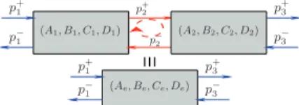
In Fig. 3 (top part), delay-free loops appear at interfaces of two systems which represent some cells of Fig. 2. These instantaneous loops cannot be simulated numerically as such, and it is necessary to remove them. To cope with this problem, it is possible to derive an equivalent two-port as the bottom of Fig. 3 shows.

p+ 1 p+ 1 p− 1 p− 1 p+ 2 p− 2 p+ 3 p+ 3 p− 3 p− 3 (A1, B1, C1, D1) (A2, B2, C2, D2)

(Ae, Be, Ce, De)

Figure 3: Concatenating two two-ports

In [11, p. 31-33], the interconnection laws are performed from

state-space representations. This leads to the matricesAe,Be,Ce

and De of the equivalent two-port. This operation is performed

recursively to remove every instantaneous loop, until the network only contains intertwined two-port systems (without delay) and

cellsQP(with delay operators).

4.2. Minimal realization

At this stage of the building, a well-known result in automatic con-trol allows to reduce the dimensions of the systems, in order to reduce the cost of numerical computation.

For an original state-space representation, the study of its ob-servability allows to know if a change of state exists, which defines observable and non-observable sub-states. From an input/output point of view it is not necessary to simulate the last substates, be-cause they have no influence on the output.

Similarly, the study of reachability allows to separate reachable and unreachable sub-states. With zero initial conditions,

unreacha-ble sub-states remain zero for bounded excitationsU .

Using the canonical Kalman’s form (cf. [19]), the minimal

re-alization is derived by eliminating non-observable or unreachable

sub-states. If they exist, the dimension of this minimal realization is lower than the original.

Remark: the minimal realization can be required for stability reasons in some particular cases (cf. eg. [20]).

4.3. Jordan decomposition

To reduce the calculation cost, it is useful to look for a new change

of state which makes the matrixA sparse.

Considering the minimal realization of a system of the

net-work, if its matrixA is diagonalizable over CJ×J_{, the modal form}

of the system is computed. If this matrix is not diagonalizable, it

always admits a Jordan decomposition over CJ×J.

Then, the appropriate change of variable is done to lead to

the new dynamics matrixA′_{with the diagonal form or the Jordan}

normal form. This matrix contains its complex eigenvalues on its

diagonal, some0 or 1 on its super-diagonal and 0 everywhere else.

4.4. Last reduction

Whereas all systems are real-valued (unandyn ∈ RN), matrices

of the state-space representation are complex-valued. From a nu-merical point of view, computation with complex numbers is more expensive than with real numbers. However using the hermitian symmetry of input/output transfer matrix (H(s) = H(s)), it is possible to reduce the number of sub-states to calculate.

The matrixA is with the Jordan normal form, then its Jordan

blocks are sorted with respect to their eigenvalues:

A′= diag(AR, AC, AC),

withARis a Jordan matrix composed with real eigenvalues,AC is

a Jordan matrix composed with complex eigenvalues with positive

imaginary part, andA_C = AC. ThenH(s) is decomposed:

H(s) = HR(s) + HC(s) + HC(s) + D.

The hermitian symmetry of H(s) and identifications prove

thatHR(s) = HR(s) and HC(s) = HC(s). Thus, the contribution

ofH_C(s) can be deduced from that of H_C(s).

Decomposing matrices with respect to eigenvalues ofA′

,B′₌ ˆ BR, BC, BC ˜T ,C′₌ˆ_C R, CC, CC ˜ andX′₌ˆ_X R, XC, XC ˜T , the equivalent scheme for simulation is, in time domain:

8 > < > : » xR(n+1) xC(n+1) – = » AR 0 0 _A C – » xR(n) xC(n) – + » BR BC – u(n), y(n) = CRxR(n) + 2ℜe “ CCxC(n) ” + Du(n). 5. RESULTS OF SIMULATIONS

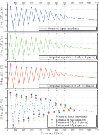
From the geometry of a real trombone, two virtual trombones are built numerically. The varying cross-section pipe of the first

vir-tual trombone,M1, is built with 11 pieces of pipe, for a refined

fit with the original shape of pipe. The second model,M2, is a

simplified version with 5 pieces of pipe. Additionally, the mouth-piece and the radiation impedance are modeled, but these models are not detailed here.

From the geometrical parameters ofM1 and M2, the

state-space representations of the networks of simulation are built with the procedures described in sections 3 and 4. These global sys-tems which represent the resonator of a trombone, have one input

and two outputs: the input is the incoming traveling wavep+

e at

the entry of the mouth-piece, and their outputs are the traveling

wavep−

e outgoing from the mouth-piece and the radiated pressure

ps from the horn. Simulating the impulse response of the input

reflexion of the resonator,p−

e/p+e, in time domain, the computed

input impedance,P/U , is deduced in frequency domain from (3).

Computed impedances are compared with the measured

impe-dance of the real trombone1in Fig. 4. As we can see, the main

im-provement of the modelM1(with 11 pieces of pipes) compared to

that ofM2(with 5 pieces) is about the spectral envelop. Whereas

the envelop of maxima and minima ofM2 is smooth, that one of

the measurements have some irregularities (see the fifth and the sixth maxima for example). With a best fit of the real shape of

pipe, the envelop ofM1has the same type of irregularities.

How-ever, because of the simplification ofM2, the complexity of the

network of simulation is reduced.

1_{Measurements was done with the impedance sensor of the Centre de}

0 100 200 300 400 500 600 700 800 900 1000 1100 −10 0 10 20 30 −10 0 10 20 30 −10 0 10 20 30 0 100 200 300 400 500 600 700 800 900 1000 1100 −10 0 10 20 30 Frequencyf (hertz) 2 0 lo g10 (| Zm (f )| ) 2 0 lo g10 (| Z1 (f )| ) 2 0 lo g10 (| Z2 (f )| ) 2 0 lo g10 (| Zk (f )| )

Measured input impedance

Computed impedance of M1(11 pieces)

Computed impedance of M2(5 pieces)

Measured input impedance Extrema of measurements Extrema of M1(11 pieces) Extrema of M2(5 pieces)

Figure 4: Comparison between impedances.

6. CONCLUSIONS AND PERSPECTIVES

Using the formalism of state-space representations for digital wave-guide networks leads to a good modularity for the assembling of elements, and an automatic building of the network of simulation. Moreover, standard tools of automatic control are used to reduce the calculation cost.

Considering the refined model of Webster-Lokshin for lossy flared pipes, it has been shown that this formalism can be applied with approximations of the diffusive representations by finite-di-mensional systems. Compared to models based on cylinders or cones, this model requires much fewer pieces of pipes to obtain good geometrical fits and realistic computed impedances.

At present, the global complexity of computation is equivalent to former models mentioned above. But the dimension of approx-imation (cf. sec. 3.1) can be reduced with a different method.

In this paper, only linear resonators with static parameters have been presented. In order to have a complete computer-aided maker of virtual wind instruments, nonlinear or time-varying system must be considered: trombone slide, valves, lips, reed, tone-holes. The modularity of the formalism should make an easy integration pos-sible with only a few differences.

7. ACKNOWLEDGMENT

The authors thank René Caussé, Thomas Hézard and Pierre-Da-mien Dekoninck for their collaboration.

8. REFERENCES

[1] J. O. Smith, Applications of Digital Signal Processing to

Audio and Acoustics, pp. 417–466, Kluwer Academic

Pub-lishers, February 1998.

[2] A. Webster, “Acoustic impedance and the theory of horns and of the phonograph,” Proc. Nat. Acad. Sci. U.S, 1919. [3] J. D. Markel and A. H. Gray, “On autocorrelation equations

as applied to speech analysis,” IEEE Trans. Audio and

Elec-troacoust., vol. AU-21, no. 2, pp. 69–79, April 1973.

[4] V. Välimäki, Discrete-time modeling of acoustic tubes using

fractional delay filters, Ph.D. thesis, Helsinski University of

Technology, 1995.

[5] D. Matignon, Représentations en variables d’état de guides

d’ondes avec dérivation fractionnaire, Ph.D. thesis,

Univer-sité Paris-Sud, 1994.

[6] E. Ducasse, “An alternative to the traveling-wave approach for use in two-port descriptions of acoustic bores,” J. Acoust.

Soc. Am., vol. 112, pp. 3031–3041, 2002.

[7] J.-D. Polack, “Time domain solution of Kirchhoff’s equa-tion for sound propagaequa-tion in viscothermal gases: a diffusion process,” J. Acoustique, vol. 4, pp. 47–67, February 1991. [8] T. Hélie, R. Mignot, and D. Matignon, “Waveguide

mode-ling of lossy flared acoustic pipes: Derivation of a

Kelly-Lochbaum structure for real-time simulations,” in IEEE

WASPAA, Mohonk, USA, 2007, pp. 267–270.

[9] T. Hélie, “Unidimensional models of acoustic propagation in axisymmetric waveguides,” J. Acoust. Soc. Am., 2003. [10] D. Matignon, “Physical modelling of musical instruments:

analysis/synthesis by means of state space representations,” in ISMA95, pp. 496–502.

[11] S. Tassart, Modélisation, simulation et analyse des

instru-ments à vent avec retards fractionnaires, Ph.D. thesis,

Uni-versité Paris VI, Paris, 1999.

[12] R. Mignot, T. Hélie, and D. Matignon, “From the Webster-Lokshin equation to a general framework for simulation of digital waveguides,” Submitted, 2009.

[13] T. Hélie, Modélisation physique des instruments de musique

en systêmes dynamiques et inversion, Ph.D. thesis,

Univer-sité Paris-Sud, Orsay, France, 2002.

[14] T. Hélie and D. Matignon, “Diffusive reprentations for the analysis and simulation of flared acoustic pipes with visco-thermal losses,” Math. Models Meth. Appl. Sci., 2006. [15] D. Matignon, “Stability properties for generalized fractional

differential systems,” ESAIM: Proc, vol. 5, 1998.

[16] O. J. Staffans, “Well-posedness and stabilizability of a vis-coealistic in energy space,” Trans. Amer. Math. Soc., vol. 345, no. 2, pp. 527–575, 1994.

[17] G. Montseny, “Diffusive representation of

pseudo-dif-ferential time-operators,” ESAIM: Proc, vol. 5, 1998. [18] G. F. Franklin, J. D. Powell, and M. L. Workman, Digital

Control of Dynamic Systems, p.151, Addison-Wesley, 1990.

[19] R. Kalman, “Canonical structure of linear dynamical sys-tems,” in Proc. of the Nat. Ac. of Sciences.

[20] R. Mignot, T. Hélie, and D. Matignon, “Stable realization of a delay system modeling a convergent acoustic cone,” in