Nonlinear Discrete Observer for Flexibility Compensation of Industrial Robots

Science Arts & Métiers (SAM)

is an open access repository that collects the work of Arts et Métiers Institute of

Technology researchers and makes it freely available over the web where possible.

This is an author-deposited version published in: https://sam.ensam.eu

Handle ID: .http://hdl.handle.net/10985/8755

To cite this version :

Jinna QIN, François LEONARD, Gabriel ABBA - Nonlinear Discrete Observer for Flexibility Compensation of Industrial Robots In: IFAC World Congress 2014, South Africa, 20140824 -Proceedings of IFAC World Congress 2014 - 2014

Any correspondence concerning this service should be sent to the repository Administrator : archiveouverte@ensam.eu

Nonlinear Discrete Observer for Flexibility

Compensation of Industrial Robots ⋆

J. Qin∗ F. Léonard∗∗ G. Abba∗∗

∗_{Design, Manufacturing and Control Laboratory (LCFC), Arts et}

Métiers ParisTech, 57078 Metz, France. (Email: jinna.qin@ensam.eu)

∗∗_{Design, Manufacturing and Control Laboratory (LCFC), National}

Engineering College of Metz, 57035 Metz Cedex, France.(Email: leonard@enim.fr),(Email: gabriel.abba@ensam.eu)

Abstract: This paper demonstrates the solutions of digital observer implementation for industrial applications. A nonlinear high-gain discrete observer is proposed to compensate the tracking error due to the flexibility of robot manipulators. The proposed discrete observer is obtained by using Euler approximate discretization of the continuous observer. A series of experimental validations have been carried out on a 6 DOF industrial manipulator during a Friction Stir Welding process. The results showed good performance of discrete observer and the observer based compensation has succeed to correct the positioning error in real-time implementation.

Keywords: Observer; Discrete-time; Flexibility compensation; Industrial robot; Real-time implementation.

1. INTRODUCTION

Observers are widely used to estimate unknown or unmea-surable variables of linear or nonlinear systems. The ob-server considered in this study is used to determine the real state (pose and twists) as well as external forces of a 6 DOF industrial robot manipulator. Under significant external forces (e.g. for Friction Stir Welding (FSW) process as first proposed by Thomas et al. [1991]), the manipulators are not rigid enough to perform the task under the process requirements. As a consequence, the deformation due to the flexibility of robot needs to be taken into account. Which means, the robot joint position is different from the one measured with the motor encoder. However, those variables are usually not measured by industrial manipula-tors. That’s the reason why we proposed an observer-based control.

In recent years, high-gain observers have been widely ap-plied in the nonlinear output feedback control of nonlinear systems. The computing problem of exact discrete-time models is a reason that makes the sampled-data nonlinear control difficult as described by Nešić and Teel [2004]. The solutions to realise the real-time implementation of discrete-time high-gain observer is highly required. Dabroom and Khalil [1999] studies discrete-time imple-mentation of high-gain observers and their use as numer-ical differentiators. They compared several discretization methods and found out that the bilinear transformation method outperforms other methods. But no general the-orem has proposed in this paper, and these methods are classically used for linear systems. The design of nonlinear

⋆ This study is a part of the project

ANR-2010-SEGI-003-01-COROUSSO that is sponsored by the French National Agency of Research as a part of the program ANR-ARPEGE.

sampled-data controllers based on approximate discrete-time models is presented in Nešić et al. [1999]. They com-pared the regions of attractions with different sampling period for different controllers using Euler or a second approximation of the plant model. This article shows that the Euler based control has a good performance with small and large sampling time and shows better performance than the Damping control.

Arcak and Nešić [2004] proposed a framework for digital controller design based on approximate discrete-time mod-els of the plant, with a nonlinear sampled-data observer to guarantee a good performance on the exact discrete-time model and pointed out that the sampling periods cannot be arbitrarily reduced in real-time applications. Moreover continuous differentiator or integrator can be numerically approached using some transformations (Aström and Wit-tenmark [1997], Franklin et al. [1998], Krishna [2011]) but for an integrator used in closed loop control Simp-son method is not recommended (see Léonard and Abba [2012]) whereas Euler method appears to be efficient as ex-plained by Nešić et al. [1999]. On the other hand, Nešić and Teel [2006] present several backstepping designs in strict feedback form based on the Euler approximate discrete-time model of a continuous-discrete-time plant as not all the backstepping controllers based on Euler approximate plan model stabilize the discrete plant. Real time experiments of industrial robots with observers have been carrying out by De Luca et al. [2007], Boukezzoula et al. [2004]. A dual-rate observer-based output feedback controller is proposed in Ustunturk [2012], which deals with the problem of output feedback stabilization of sampled-data nonlinear systems under the constraint of low measurement rate. A numerical example is given in this paper to illustrate the

proposed method.

The objective of this paper is the design of a high gain nonlinear discrete observer using Euler approximation of the continuous high gain nonlinear observer proposed by Qin et al. [2013] in order to build the joint state of flexible industrial robots. The estimation of this state enables us to compensate the flexibility of these manipulators in real time. Such a compensation can be carried out for industrial processes like manufacturing as described by Qin et al. [2012].

This paper is organized as follows: In Section 2 the modelling of an industrial robot manipulator is presented. In Section 3 the design of nonlinear continuous high-gain observer proposed by Qin et al. [2013] is briefly reminded. Section 4 proposes the design of the new discrete high gain observer with its proof of stability. Then Section 5 provides the results of experiments with an industrial robot Kuka KR500-2MT used for a welding process. These results show good performances of the proposed digital observer. Finally, conclusions and ideas for future work are discussed in Section 6.

2. MODELING OF FLEXIBLE JOINT ROBOT The robot concerned in this study is a serial chain ma-nipulator (see Fig. 1). The control problem of this kind of manipulator for precise manufacturing is a challenging task: the manipulator is an elastic multibody, multivari-able and strongly coupled system. Its highly non-linear dynamics change rapidly while manipulator moves in its workspace.

Fig. 1. Robot KUKA KR500-2MT (by courtesy of Institut de Soudure)

The Modified Denavit-Hartenberg (MDH) notation is fre-quently used to model robots including the robot con-cerned in this research work Khalil and Dombre [2004]. The MDH parameters for this manipulator are listed in Table 1 and are used for the modeling of robot with the help of software SY M ORO+ Khalil and Creusot [1997].

Fig. 2. Modelisation of robot

The Fig. 2 shows a general model of the robot manipulator. By choosing distance Dt and angle αt, this model can be adapted for different tools when the rotation axis of the tool has an offset or if not coaxial with axis 6. More details can be found in Qin [2013] such as, for instance, the rigidity of each axis.

Table 1. MDH paramètres du robot rigide

j µj σj αj dj θj rj 1 1 0 π 0 q1 −L1z 2 1 0 π/2 L1x q2 0 3 1 0 0 L2 π/2 + q3 0 4 1 0 −π/2 D4 q4 −L34 5 1 0 π/2 0 q5 0 6 1 0 −π/2 0 q6 −L5 7 0 2 0 −Dt −π/2 0 t 0 2 αt 0 0 −Ltz

According to Spong et al. [2005], a dynamic model of a flexible joint robot can be expressed as follows:

D(q)¨q = Γ− H(q, ˙q) − Ff r( ˙q)− JT(q)F (1)

Iaθ = Γ¨ m− NvTΓ− Ff m( ˙θ) (2) where JT_(q)

(6×6) is the Jacobian matrix of the tool frame, F(6×1) is the wrench vector applied by robot on external environment, Γm(6×1) is the vector of mo-tor mo-torques, Γ is the vecmo-tor of gearbox mo-torque, vecmo-tors

q = [q1q2q3q4q5q6]T, ˙q and ¨q represent angular posi-tions, velocities and acceleraposi-tions, respectively. Vectors

θ = [θ1θ2θ3θ4θ5θ6]T, ˙θ and ¨θ denote the vector of an-gular positions, velocities and accelerations of motor axes, respectively. Here Nv = N−1 is the gear transmissions ratio matrix. For the robot Kuka KR500-2MT, N is not a diagonal matrix, there is also a coupling among axes 4, 5 and 6. D(q) is the symmetric, uniformly positive definite and bounded inertia matrix of the robot. Ia is the inertia matrix of the motor. H(q, ˙q) represents the

contribution due to centrifugal, Coriolis and gravitational forces and the gravity compensator of axis two. Ff r and

Ff m are vectors of the friction at joint and motor axis respectively. Robots have two main sources of flexibilities: the flexibilities of body/arms, and those located at joints (which include those of motors and transmissions). Here-after, links of robot are considered as rigid and only the

flexibilities localized at gearboxes are taken into account and represented by a rigidity matrix K:

Γ = K(Nvθ− q) (3)

3. NON LINEAR CONTINUOUS HIGH GAIN OBSERVER FOR FLEXIBLE ROBOTS

Fig. 3. Non linear continuous high gain observer design proposed by Qin et al. [2013]

In this paragraph, the design of nonlinear continuous high-gain observer proposed by Qin et al. [2013] is summarized since it will be emulated in the next paragraphe. If we define the measured variables as y, according to equations (1), we obtain:    z1= [Ia−1N−TK]−1x4= K−1NTIaθ˙ z2= q , z3= ˙q , z4=−D−1(z2)JT(z2)F y1= θ , y2= ˙θ (4) Moreover, if u = Γmthen:          ˙ z1= z2+ K−1NT[u− Ff m(y2)]− Nvy1 ˙ z2= z3 ˙ z3= z4+ ψ(z2, z3, y1) ˙ z4=− d dt[D −1_(z 2)JT(z2)F ] (5)

where ψ is equal to:

ψ = D(z2)−1[K(Nvy1− z2)− H(z2, z3)− Ff r(z3)] (6) If A and C are defined as following (for a robot with n axes, I is the n order identity matrix and 0 is the n× n zero matrix): A =    0 I 0 0 0 0 I 0 0 0 0 I 0 0 0 0    and C = (I 0 0 0) (7) then: ˙ z = Az + g(z, y, u) + d(z, F, ˙F ) (8) with g =      K−1NT[u− Ff m(y2)]− Nvy1 0 ψ(z2, z3, y1) 0 (9) and d(z, F, ˙F ) = [0 0 0 −_dtd[D−1(z2)JT(z2)F ]]T. Define now the following high gains matrix, with G a constant≥ 1: ΓG=     GI 0 0 0 0 G2I 0 0 0 0 G3I 0 0 0 0 G4I     (10)

and matrix L such as (A− LC) has all its eigenvalues in the left half of the complex plane, then a new observer is proposed as follow: ˙ˆz = (A − ΓGLC)ˆz + g(¯z, y, u) + ΓGKy¯ 2 (11) where ¯K = LK−1NTIa and:              ¯ z2= Nvy1− Nvy1− ˆz2 ∥ Nvy1− ˆz2∥ Nssat(∥ N vy1− ˆz2∥ Ns ) ¯ z3= ˆ z3 ∥ ˆz3∥ Mssat( ∥ ˆz3∥ Ms ) ¯ z4= ˆ z4 ∥ ˆz4∥ Assat(∥ ˆz 4∥ As ) (12)

with the function of saturation:

sat(x) =

{

x if | x | ≤ 1

1 if | x | > 1 (13) and Ms, Ns, FM, Fd, JM, DM and Asare known positive physical constant bounds:

{

∥ x2∥< Ms,∥ x1− x3∥< Ns,∥ F ∥< FM,∥ ˙F ∥< Fd

∥ JT_(z

2)∥< JM,∥ D−1(z2)∥< DM, As= DMJMFM Fig. 3 shows the diagram of the proposed observer where

Ac = A− ΓGLC. For only one axis, L = [L1L2L3L4]T and:

det[λI− (A − LC)] = λ4+ L1λ3+ L2λ2+ L3λ + L4 (14) where λ is an eigenvalue of matrix A− LC. A possible choice for L is then: L1 = 4a, L2 = 6a2, L3 = 4a3 and

L4 = a4. In this case, matrix A− LC has four stable eigenvalues in λ =−a, where a is a positive real fixing the dynamics of the proposed observer.

The estimation error e = z − ˆz satisfies the following differential equation:

˙e = Ace + g(z, y, u)− g(¯z, y, u) + d(z, F, ˙F ) (15) Because of the form of disturbance d(z, F, ˙F ) the following

stability theorem can be proven for the observer (11) (see Qin et al. [2013]):

Theorem 3.1: There exists a constant G0_{such that error}

e(t) is bounded for any gain G > G0_.

4. NONLINEAR HIGH-GAIN DISCRETE OBSERVER DESIGN

Fig. 4. Discrete observer design

High-gain observers are important for the output feedback control of nonlinear systems and they are almost always implemented digitally in industrial applications. However, many studies have been limited to continuous-time analy-sis Dabroom and Khalil [1999]. In this paragraph, a nonlin-ear high-gain discrete observer is proposed to compensate

the errors due to the flexibilities of industrial robots. Such robot flexibilities induce large position errors in case of processes which need high supply force like for instance FSW process as described by Zhao et al. [2009]. As the continuous observer is nonlinear, a good compromise is ob-tained using only a first order approximation like Euler one as for nonlinear system high order discrete approximations are usually very complex and not really more significantly accurate, Nešić et al. [1999]. The proposed discrete ob-server is obtained using Euler approximate discretization of the continuous observer (11) where T is the sampling time of the discrete observer:

ˆ

z(k + 1) = ˆz(k) + T (Acz + g(¯ˆ z(k), y(k), u(k)) + KGy2(k)) (16) where KG= ΓGK. Relation (16) can be factorized as:¯ ˆ

z(k+1) = (I +T Ac)ˆz(k)+T (g(¯z(k), y(k), u(k))+KGy2(k)) (17) where I is here the twenty-four order identity matrix. This discrete observer provides naturally a good estimation of the robot state if the sampling time T is quite small, in this case a good emulation of continuous observer (11) is obtained. Unfortunately, as in (Ustunturk [2012]), the measurements and also here the control input u are only available every Tm: typically, for the Kuka robot controller KRC2 using RSI and control force tools, Tm is equal to 12 ms, Qin [2013]. To overcome this large value Tm, an linear interpolation of measure vector y and control u is done (see Fig. 4) so as the discrete observer (17) is fed at a small sampling time T = Tm/n where n is an integer design parameter chosen to get an accurate and stable digital observer. In this paper, k is used for sampling time T and k′ for sampling time Tm. To analyse stability of discrete observer (17) is convenient to introduced the matrix AT and the new input v as follows:

AT = I + T Ac (18)

v(k) = T (g(¯z(k), y(k), u(k)) + KGy2(k)) (19) so as the discrete observer (17) appears now as a linear observer with an input vector v:

ˆ

z(k + 1) = ATˆz(k) + v(k) (20) Moreover, the input u is bounded, for instance in industrial robots the motor currents are limited and the measure output y is also bounded since robot positions and speeds are also limited. On the other hand, ¯z(k) is bounded by

relation (12) and as g(¯z(k), y(k), u(k)) is only function of

sines, cosines and bounded values ¯z(k), y(k) and u(k) it

is clear that the input v(k) is bounded for any k by T ν where ν is a positive real:

||v(k)|| < T ν (21) It then appears that ||v(k)|| tends to zero when T tends to zero.

Now the following theorem shows that the state of the discrete observer (17) is bounded if the sampling time T is small enough:

Theorem 4.1: If F = A− LC is the Hurwitz matrix chosen to stabilize the continuous observer (11) and if the sampling time T is such as supi=1,24(|1 + T Gλi(F )|) < 1, where λi(F ) is the ith eigenvalues of matrix F , then the state of the digital observer (17) is bounded for any finite initial state ˆz(0).

Proof : Evolution of state ˆz(k) can be recursively obtained

using relation (20): ˆ z(k) = Ak_Tz(0) +ˆ k−1 ∑ i=0 A(k_T−i−1)v(i) (22)

Now, it is known that for a given matrix AT and ϵ > 0, there exists an induced norm matrix||.|| such that:

||AT|| ≤ ρ(AT) + ϵ (23) where ρ(AT) is the spectral radius of matrix AT. Moreover the eigenvalues of matrix AT are such that:

λ(AT) = 1 + T λ(Ac) (24) since det(AT − λI) = det(T Ac − (λ − 1)I). On the other hand, if L = [L1 L2 L3 L4]T and if, λ and λ′ are respectively an eigen value of matrix F and Ac then they are solution of respectively:

det(I6λ4+ L1λ3+ L2λ2+ L3λ + L4) = 0 (25)

det(I6λ′4+ L1Gλ′3+ L2G2λ′2+ L3G3λ′+ L4G4) = 0 (26) where I6 is the identity matrix of order 6. Multiply then equation (26) by G−4 and replace λ′G−1 by w leads to:

det(I6w4+ L1w3+ L2w2+ L3w + L4) = 0 (27) which is the same characteristic equation that the equation (25). This means that:

λ(Ac) = Gλ(F ) (28)

Reporting now equation (28) in (24) provides the following eigen value relation:

λ(AT) = 1 + GT λ(F ) (29)

which enables us to calculate the spectral radius of matrix

AT:

ρ(AT) = supi=1,24(|1 + GT λ(F )|) (30) By hypothesis supi=1,24(|1 + GT λ(F )|) < 1 so that:

0 < ρ(AT) < 1 (31) Now choosing a positive real ϵ = 0.5(1− ρ(AT)) and using norm (23) prove that:

||AT|| ≤ δ < 1 (32) where δ = 0.5 + 0.5ρ(AT), and for any integer n:

||An

T|| ≤ ||AT||n< δn< 1 (33) Finally taking norm (23) of equation (22) provides a bound for state ˆz(k): ||ˆz(k)|| ≤ ||Ak Tz(0)ˆ || + || k−1 ∑ i=0 A(k_T−i−1)v(i)|| (34) ≤ ||Ak T|| ||ˆz(0)|| + k−1 ∑ i=0 ||A(k−i−1) T || ||v(i)|| (35) Now using (33) and (21) give:

||ˆz(k)|| ≤ ||ˆz(0)|| + T ν k−1 ∑ i=0 δ(k−i−1) (36) As ∑k_i=0−1δ(k−i−1) ₌∑k−1 i=0 δ i ₌ 1− δ k 1− δ and 0 < δ < 1 it appears that: k−1 ∑ i=0 δ(k−i−1)< 1 1− δ (37)

and therefore that:

||ˆz(k)|| ≤ ||ˆz(0)|| + T ν

which proves that the state of digital observer (17) is bounded.

To get a robust digital high gain observer it is found out in Dabroom and Khalil [1999] that it is preferable to assign the poles as real ones. For instance, if twenty-four real stable poles in −a are designed for the continuous observer then theorem 4.1 guaranties the stability of digital observer (17) for:

|1 − T Ga| < 1 (39) which imposes the following practical relation to well define the sampling time T:

T < 2

Ga (40)

The sampling time T should be chosen less than bound (40) in order to get a best stability robustness as, for instance, the zero holders always provide a phase lag (see Léonard [1999]).

5. REAL TIME ROBOT FLEXIBILITY COMPENSATION USING THE PROPOSED

DISCRETE OBSERVER

The proposed discrete observer is carried out with the industrial robot Kuka KR500-2MT of Institut de Soudure in Goin, France. This robot is used for a Friction Stir Welding operation of Aluminium alloys. Table 2 shows the welding condition during the experiments.

Table 2. Table of the welding test conditions

Parameters Name/Value Unit

material Al6082

depth of welt piece (dm) 6 mm

advance speed (va) 400 mm/min

rotation speed (Ω) 1100 rpm

desired axial force (Fzd) 9000 N

The robot is controlled in force in its z direction (9000 N desired) and a welding in its x direction with an advance speed va is programmed. An external computer receives each Tm = 12 ms the joint positions and the currents of each robot axis. In the external computer, the digital observer (17) is implemented as a C++ program with the sampling time T = Tm/n. Each period Tm, the computer sends to robot via an Ethernet link a trajectory correction ∆Y (k′) in order to compensate the positioning error in

y-direction due to the robot flexibility. In fact, the robot

flexibility error vector ∆P (k′) can be evaluated as (see Qin [2013]):

∆P (k′) = J (ˆq(k′))(ˆq(k′)− N−1θ(k′)) (41) = [∆X(k′) ∆Y (k′) ∆Z(k′) ∆θx(k′) ∆θy(k′) ∆θz(k′)]T

(42) To appreciate accuracy of proposed digital observer, the observer error ˆe is calculated as:

ˆ

e(k) = ˙θl(k)−θˆ˙l(k) = ˙θl(k)− N−1Ia−1N−TK ˆz1 (43) and its RMS value is obtained as:

ˆ ERM S = v u u t(1/6)∑6 i=1 ˆ eRM S(i)2 (44)

where ˆeRM S(i) is the RMS observer error of axis i during the welding. For the welding, the twenty-four continuous

observer poles are chosen in−a with a = 52 and G = 1. In this case, the sampling T should be less than 2/(Ga) = 38.5 ms as described by (40). Nevertheless, a smaller value must be used to get a certain stability margin. Thus Table 3 shows that if n is greater or equal to 4, a constant and very small value of ˆERM S is got. For n = 1, i.e.

T = 12 ms, the proposed digital observer is stable but

has a bad accuracy. Moreover, a too large value of n needs more calculation time and also a large mantissa for the different variables used by discrete observer. These results are obtained without compensation of the robot flexibility i.e. ∆Y (k′) send by external computer to Kuka robot are null. Fig. 5 displays digital observer error for n = 10, this means that the digital observer state is calculated every

T = 1.2 ms although the robot positions and currents are

only received by external computer every Tm= 12 ms. It can be noticed in this figure that a persistent very small static error exists for each axis, which is not surprising as the proposed digital observer is not an exact one. Such an static error exists even for very small sampling time as mentioned in Arcak and Nešić [2004].

A FSW welding has also been carried out using compen-sation ∆Y (k′) calculated by relation (41).

Table 3. RMS observer error ˆERM S(mrad/s) versus n = Tm/T n 1 2 3 4 5 10 1000 ˆ ERM S 3.2106 3.0106 0.47 0.46 0.46 0.46 0.46 0 1 2 3 4 5 6 7 8 9 10 −2.5 −2 −1.5 −1 −0.5 0 0.5 1 1.5 2 2.5x 10 −3 t [s] Error [rad/s] axis1 axis2 axis3 axis4 axis5 axis6

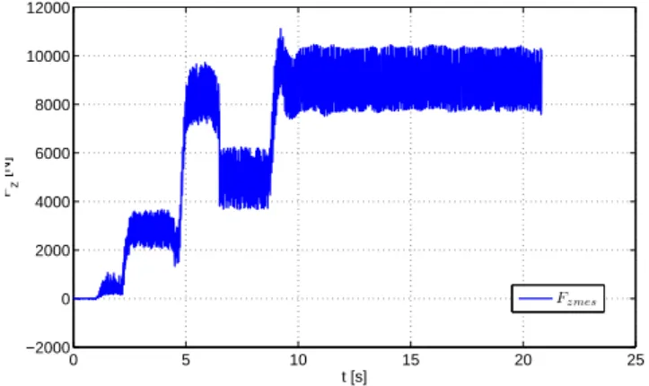
Fig. 5. Digital observer error of velocities for n = 10 The results of FSW in this paper are obtained from the test IS1709J. The dive phase consists of three levels of force of 600 N , 3000 N and 9000 N in z direction. In Fig. 6, one can see the three different force level set points and that in the welding phase a mean force of 9000 N is effective with a variation of±1000 N at a frequency close to the tools rotation speed (1100 rpm). Then at t = 7.7 s, the derivative of the lateral adjustment ∆Y (k′) calculated by the digital observer is sent to robot which corrects its trajectory in relative mode every 12 ms. At t = 8.8 s , the force controller is reactivated in z direction with a set point of 9000 N and a movement in x direction is begun with an advance speed of 400 mm/min (see Table 2). Once this displacement is effected, the force control

is deactivated and the PC-robot connection is cut. Fig. 9 shows the welded work-piece where one can see that the robot can weld the work-piece in a desired location with the help of discrete compensator (41). Without this discrete compensation a static error of about 4.8 mm in y position could be observed that means than the proposed discrete compensator suppress more than 90 % of error in y direction. Fig.7 shows the correction ∆Y (k′) calculated by external computer, a static correction of 4.8 mm is effective using the proposed discrete observer. We can also see the current of each joint in Fig. 8 and notice that during the welding phase, the axes 2 and 3 are the most requested.

0 5 10 15 20 25 −2000 0 2000 4000 6000 8000 10000 12000 t [s] Fz [N] Fz mes

Fig. 6. Measured axial force

0 5 10 15 20 25 0 1 2 3 4 5 t [s] ∆Y [mm] 0 5 10 15 20 25 −0.04 −0.02 0 0.02 0.04 t [s] ∆Y (k) − ∆Y (k−1)[mm] ∆Y d_∆Y

Fig. 7. Calculated absolute correction ∆Y and relative real time correction ∆Y (k′)−∆Y (k′−1) sent to the robot during the FSW operation

6. CONCLUSION

This paper proposed a new discrete high gain observer to calculate the state of flexible industrial robots. A theorem is proposed to guarantee its stability. This new discrete observer is obtained by emulation of the observer intro-duced by Qin et al. [2013] by using Euler approximation. This discrete observer has been implemented in C++ in an external computer and it has proven to be effective for FSW process done with an industrial robot. More precisely, with the discrete compensation (41), more than

0 5 10 15 20 25 −10 −5 0 5 10 15 20 t [s] Current [A] I1 I2 I3 I4 I5 I6

Fig. 8. Measured currents sent by Kuka Controller used as the entry of digital observer

Fig. 9. Welded work-piece with compensation

90 % of error due to the Kuka KR500-2MT robot flexibility has been cancelled in a FSW process with a significant external force for this robot. In this application, a sampling time T = 1.2 ms is used to calculate the state of the discrete observer whereas the input of observer has fed only with a sampling time of Tm= 12 ms. Such a result proves also that industrial robot flexibility can be compensated in real time, which opens the door to many new process robotization that needed very important force supply or a better precision.

ACKNOWLEDGEMENTS

The authors would like to thank the partner of project, Institut de Soudure. Especial thanks to Thomas Goubet for his support during the experimental validation.

REFERENCES

M. Arcak and D. Nešić. A framework for nonlinear sampled-data observer design via approximate discrete-time models and emulation. Automatica, 40(11):1931– 1938, 2004.

K. J. Aström and B. Wittenmark. Computer controlled

systems. Prentice Hall International, 1997.

R. Boukezzoula, S. Galichet, and L. Foulloy. Observer-based fuzzy adaptive control for a class of nonlinear systems: real-time implementation for a robot wrist.

Control Systems Technology, IEEE Transactions on, 12

(3):340–351, May 2004.

A.M. Dabroom and H.K. Khalil. Discrete-time implemen-tation of high-gain observers for numerical differenti-ation. International Journal of Control, 72(17):1523– 1537, 1999.

A. De Luca, D. Schroder, and M. Thummel. An acceleration-based state observer for robot manipulators with elastic joints. In IEEE International Conference

on Robotics and Automation, pages 3817–3823, Roma,

Italy, May 2007.

G. F. Franklin, J. D. Powell, and M. L. Workman. Digital

Control of Dynamic Systems. Addison Wesley, 1998.

W. Khalil and D. Creusot. Symoro+: A system for the symbolic modelling of robots. Robotica, 15:153–161,

1997.

W. Khalil and E. Dombre. Modeling, Identification and

Control of Robots. Elsevier Ltd, Oxford, 2004.

B. T. Krishna. Studies on fractional order differentiators and integrators : A survey. Signal Processing, 91:386– 426, 2011.

F. Léonard. First-order optimal reduced-delay sample-data holds. IEEE Trans. Autom. Control, 44(7):1446– 1448, 1999.

F. Léonard and G. Abba. Robustness and safe sampling of distributed-delay control laws for unstable delayed systems. IEEE Trans. Autom. Control, 57(6):1521–

1526, 2012.

D. Nešić and A.R. Teel. A framework for stabilization of nonlinear sampled-data systems based on their ap-proximate discrete-time models. IEEE Transactions on

Automatic Control, 49(7):1103–1122, 2004.

D. Nešić and A.R. Teel. Stabilization of sampled-data nonlinear systems via backstepping on their euler ap-proximate model. Automatica, 42(10):1801–1808, 2006. D. Nešić, A.R. Teel, and P.V. Kokotović. Sufficient condi-tions for stabilization of sampled-data nonlinear systems via discrete-time approximations. Systems Control

Let-ters, 38:259–270, 1999.

J. Qin. Robust Hybrid Position/Force Control of a

Ma-nipulator Used in Machining and in Friction Stir Weld-ing(FSW). Phd thesis, ENSAM, Metz, France, 2013.

J. Qin, F. Léonard, and G. Abba. Non-linear observer-based control of flexible-joint manipulators used in ma-chine processing. In Proceedings of The ASME 2012

11th Biennial Conference on Engineering Systems De-sign and Analysis, number 82048, Nantes, France, July

2012.

J. Qin, F. Léonard, and G. Abba. Experimental external force estimation using a non-linear observer for 6 axes flexible-joint industrial manipulators. In The 9th Asian

Control Conference, pages 701–706, Istanbul, Turkey,

June 2013.

Mark W. Spong, Seth. Hutchinson, and M. Vidyasagar.

Robot Modeling and Control. John Wiley and Sons, Inc.,

Berlin Heidelberg, 2005.

W. M. Thomas, E. D. Nicholas, J. C. Needham, M. G. Murch, P. Temple-Smith, and C. J. Dawes. Interna-tional patent application pct/ gb92/02203 and gb patent application. Technical report, The Welding Institute, London, UK, 1991.

A. Ustunturk. Output feedback stabilization of non-linear dual-rate sampled-data systems via an approx-imate discrete-time model. Automatica, 48(8):1796–

1802, 2012.

X. Zhao, P. Kalya, R G. Landers, and K. Krishnamurthy. Empirical dynamic modeling of friction stir welding processes. Journal of Manufacturing Science and