is an open access repository that collects the work of Arts et Métiers Institute of
Technology researchers and makes it freely available over the web where possible.
This is an author-deposited version published in: https://sam.ensam.eu Handle ID: .http://hdl.handle.net/10985/8500
To cite this version :
Joffrey VIGUIER, Arnaud JEHL, Robert COLLET, Laurent BLERON, Fabrice MERIAUDEAU Improving strength grading of lumber by grain angle measurement and mechanical modeling -Wood Material Science and Engineeering p.24 - 2015
Any correspondence concerning this service should be sent to the repository Administrator : archiveouverte@ensam.eu
Improving strength grading of timber by grain angle
measurement and mechanical modeling
Joffrey VIGUIER1*, Arnaud JEHL2, Robert COLLET2, Laurent BLERON1, Fabrice MERIAUDEAU3
Université de Lorraine, ENSTIB / LERMAB, 27 rue Philippe SEGUIN, BP1041 F-88051 Epinal Cedex 9 France
Phone: +33 (0)3 29 29 61 76 - Fax: +33 (0)3 29 29 61 38
2LaBoMaP, Groupe Matériaux et Usinage Bois, Arts & Métiers ParisTech, rue Porte de Paris F-71250 Cluny, France
3UMR 5158 uB-CNRS, Le2i, IUT du Creusot, 12 rue de la Fonderie F-71200 Le Creusot, France.
Running headline: Mechanical modeling of timber. *Corresponding author: joffrey.viguier@univ-lorraine.fr
Abstract - Timber strength grading has become a major issue in the European Union during the last years, due
to the introduction of the Eurocode 5 and all its related standards. Currently, the most performing strength grading machines are able to locally detect the boards’ knots sizes and positions and interpret this information through adapted grading models. The best lead to improve their accuracy seems to be the introduction of new information about the boards and adapt the mechanical model to take them in account. Small grain angle causes high reduction of clear wood’s mechanical properties, local value of slope of grain appears to be of high interest. The aim of this study is to quantify the additional accuracy that grain angle information can bring to an optical scanner used as a strength grading machine. A specific grading model has been developed accordingly, and the results obtained for different machine / model / loading combinations are presented. These results show that slope of grain measurement can significantly improve the accuracy of the optical scanner, for both MOE and MOR estimations.
Keywords: grain angle / spruce / strength grading / X-ray
List of symbols
ρ: Board (average) density
E: Experimental modulus of elasticity σt:Experimental tension strength σm:Experimental bending strength
MOE: Corrected modulus of elasticity taken as reference MOR: Corrected modulus of rupture taken as reference IP MOE: Indicating property of MOE
IP MOR: Indicating property of MOR
Edyn: Modulus of elasticity measured by E-Scan ECW : Modulus of elasticity of clear wood Ep: Modulus of elasticity along the profile Eb: Modulus of elasticity of the board σp: Strength of the profile
σb: Strength of the board
Ip: Quadratic momentum of the profile Ib: Quadratic momentum of the board
1
Introduction
1.1 Timber variability
The design of structures usually requires the knowledge of three points. The first one is the combination of loads that will be applied on the final structure, the second is the material that will constitute the structure and its mechanical properties, and the last one is the limits of acceptable stresses and strains. Since March 2010 in the European Union, the first and last points are regulated by the Eurocode 5 and its associated standards. The second one, however, is supposed to be provided by the material’s supplier. Apart from timber, structures can usually involve concrete and steel. On the opposite of these materials, whose raw materials and manufacturing processes are controlled, the growth of the trees is led by multiple factors on which foresters have little influence. As a result, wood presents a very high variability degree due to the growth conditions, and to the presence of local singularities which have a direct influence on boards’ mechanical properties. This makes a statistical characterization of timber impossible within a single species, a single growth area, and even a single tree. In order to harmonize the structures design methods, the EN338 standard (AFNOR, 2009) defines a set of strength classes, which imposes limits on the boards’ mechanical properties. Consequently each board must be affected to the appropriate grade. Regardless of the standardized process, the objective of strength grading is to define Indicating Properties (IPs) of each board describing its density, mean Modulus of Elasticity (MOE) and Modulus of Rupture (MOR).
1.2 Strength grading technologies
The strength grading machines technologies can be divided into two groups. The first ones uses the rather high correlation between timber’s MOE and its MOR , and proceed to the MOE measurement either by a vibration analysis , or a dynamic and non-destructive bending test. According to the method used for the modulus’s measure, several studies showed that the coefficients of determination between MOE and MOR are limited to 0.70 (Hanhijärvi et al., 2005; Rohanovà et al., 2011). This method is currently the most commonly applied in the industry thanks to its simplicity and relatively low cost. However, this technology remains limited due to its incapacity to take local singularities in account. In addition, these machines’ performances rely mostly on the species mechanical properties correlations, and are not suitable for boards optimization applications. The other strength grading technology consists in using an optical scanner to detect local singularities and integrate them in the grading model. Usually, the singularities of interest are knots, detected either by an X-Rays sensor, or by laser imaging, then matched using an appropriate algorithm (Roblot et al., 2008). The knots sizes and positions
information is then summarized in the Knots Area Ratio (KAR) indicator or one of its variants, which are proven to be well correlated to the boards’ MOR . Apart from knots, several kinds of singularities are known to be strength reducing, especially the angle between fibers and stress respective directions, called grain angle . Several studies have already shown that mean grain angle is correlated to boards’ mechanical properties (Pope et al., 2005; Brännström et al., 2008). Baño et al. (2011) also showed that the association of slope of grain and nodosity measurements in a finite element model, conducts to a high correlation between experimental and predicted bending strength (R2=0.88). The consideration of the slope of grain appears to be effective, but finite element method is not industrially applicable because of the computational time.
1.3 Objectives
The main objective of this study is to determine if local grain angle measurement can potentially improve the performances of optical scanners as strength grading machines. Estimations of MOE and MOR using this equipment (combined or not to a vibrations analysis device to measure the boards’ dynamic MOE) have been performed with current X-Ray imaging technologies only, or with additional local grain angle information. The results, in terms of determination coefficients between predicted and destructively measured mechanical properties, have then been compared in the different configurations. In addition, since current grading models are not natively designed to take in account additional data, a new and adapted model has been developed, and is presented below.
2
Materials and methods
2.1 Samples description and destructive tests
The batch of samples used in this study is constituted by 1373 boards of European spruce (Picea abies). All of them are 4m in length and the range of cross-sections is described in Table 1. The different boards have been dried to around 12% of moisture content. Among all of these boards, 1017 have been destructively tested in bending and 356 have been tested in tension. These destructive tests have been performed according to both EN 408 (AFNOR, 2012) and EN 384 (AFNOR, 2010). The critical cross-section was chosen visually and placed between the loading heads in bending or between the jaws in tension. In tension, the boards were gripped by jaws on both endings and the critical-cross-section was located in a range of 9 time the specimen’s width. Bending tests were performed using a distance equal to 18 times the specimen’s width between the supports and
6 times between the loading heads. The bending test performed is an edgewise bending test and the tension edge was selected at random.
According to EN 384 (AFNOR, 2010) some adjustments have been made on measured values of modulus of elasticity in bending and both tension and bending strength. MOE has been converted using equation 1 where E is the measured global modulus of elasticity and MOR by equation 2 where σt and σm are respectively the measured strength in tension and in bending in order to normalize the strength to boards of 150mm of width.
MOE = 1.3 ∙ E − 2690 (1)
= ( ℎ 150)⁄ .
( !) (2)
2.2 Data acquisition and processing
2.2.1 X-Ray densitometry
The CombiScan+ optical scanner produced by Luxscan Technologies can be equipped with an X-Rays imaging system. Assuming that the grey levels of thereby provided images are proportional to the acquired corresponding light intensities, they can be easily and accurately converted into local densities maps. Under this condition, the Beer-Lambert’s law was applied, which describes the intensity of an electromagnetic field crossing a homogeneous material layer. In our case, the final expression of the local density ρ, averaged through the board’s thickness, is given by the equation 3, where t represents the board’s thickness, a and b are linear calibration coefficients, and G is the corresponding image pixel’s grey level.
t ∙ ρ(x, y) = a ∙ ln(G)(+,,)+ b (3)
The actual values of a and b depend on a lot of factors but can easily be quantified by scanning and weighing a batch of boards. These two parameters are then defined as the linear regression coefficients (see Figure 6) between the board’s mean values of ln(G) calculated on the images and their mean densities multiplied by their respective thickness measured manually.
Despite the contactless nature and the high speed of X-Ray densitometry, the random estimation error remains reasonably low. Its 99% confidence interval has been measured to less than 5%, which is equivalent to the accuracy of an on-the-run weighing system.
The real interest of this method stands in its ability to provide a local density measurement, and therefore to highlight the presence of knots (Figure 1). With its help, it is possible to estimate the Knots Depth Ratio (KDR), which represents the local knot thickness divided by the board’s one (Oh et al., 2009). A first image processing step is used to separate knotty areas to clear wood ones, and the average clear wood density (ρCW) can consequently be determined. For each board, it was assumed that knots density (ρKN) is constant and proportional to ρCW (Oh et al., 2009). Finally, the local KDR value is defined by the equation 4, and will be later used in our strength grading model.
KDR(x, y) = ρ(+,,)2 ρ34
ρ56 2 ρ34 (4)
2.2.2 Dynamic MOE
The boards’ MOE has been measured with E-Scan, a product of Luxscan Technologies. This vibration analysis system is made up of a hammer, hitting one end of the board, inducing the propagation of a tension/compression wave. Displacements at the end of the board are measured with a laser interferometer, and then a Fourier transform is applied on the output signal in order to determine its main frequency (f0). The equation 5 defines the relationship between this frequency, the board’s dynamic modulus of elasticity (Edyn), its density (ρ), and its length (L) .
E7,8 = ρ ∙ (2Lf )² (5)
The boards mean densities can either be measured by an additional weighing station, or by X-rays densitometry if combined to a CombiScan+ scanner. Both methods give similar results in terms of accuracy and reliability, but we chose the second one for more convenience (see part 3.2).
2.2.3 Grain angle
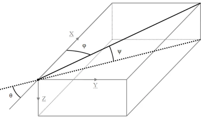
The angle θ between the fibers direction and the board’s main axis is the combination of two angles that we called φ and ψ. The projection angle φ stands between the board’s axis and the projection of the fibers direction on the observed face, whereas ψ represents the diving angle between the fibers direction and the observed face. In other terms φ is the projection of grain angle in the X-Y plane axis whereas ψ is the one in the X-Z plane. All these angles are represented in Figure 2.
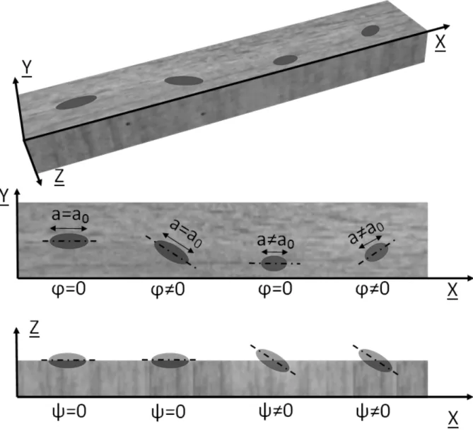
The optical scanner’s grain angle measurement device produced by Luxscan Technologies and integrated in the CombiScan+ uses the so-called tracheid effect (Simonaho et al., 2004; Nyström, 2003; Hu et al., 2004), which consists in projecting a dot laser perpendicularly on the top and bottom faces. The grain angle is measured on top and bottom faces at the same time. This measurement was made on both sides of the 1373 rough sawn timber. As a result of wood’s anisotropic light diffusion properties, one can observe an elliptic light pattern oriented parallel to the projection of the fibers axis on the observed surface (Figure 3). Consequently, the measure of the projection angle (φ) can be obtained thanks to a Principal Component Analysis applied on the ellipse binarized image (Simonaho et al., 2004; Nyström, 2003). The bottom part of Figure 3 shows how the eccentricity is calculated by measuring the length of the two axes constitutive of the ellipse. In addition to the projection angle (φ), the ellipses also contain an indication of the diving angle (ψ), which appears to be linked to their shape factor. In order to be able to calculate this angle, it was assumed that wood presents orthotropic light diffusion properties, similarly to (Simonaho and Silvennoinen, 2004; Kienle et al., 2008). Under this assumption, the Figure 4 illustrates a side view of the tracheid effect, where the visible ellipse pattern is the intersection between the observed face and a spheroid oriented parallel to the grain direction.
With the application of the polar coordinates ellipse equation, (equation 6) the angle ψ can be determined, where a and b are respectively the detected ellipse’s major and minor axis. The e0 parameter is defined as the eccentricity of the ellipse pattern if the diving angle was equal to 0. In practice, this parameter cannot be measured and it is taken as the 20% fractile of the measured eccentricity for each line of laser dots along the board. This value is determined in order to optimize the coefficient of determination. The assumption made here is that the diving angle is more often equal to 0 due to the extraction way of the board from the trunk.
a² = < – >?²;² @AB²(C) (6)
The next step in determining the actual grain angle θ corresponding to one ellipse is to merge the projection and diving angle information, according to the equation 7. Finally, grain angle values between two consecutive dots in the Y direction and values of θ between top and bottom faces are estimated by linear interpolation between grain angles values at the corresponding (x,y) positions. The resolution in x and y directions is respectively 10 and 3 mm. This constitutes the highest hypothesis of this model, and the resulting estimation errors will later be studied.
2.3 Mechanical modeling
The mechanical modeling consists of using the data previously acquired ρ(x,y), KDR(x,y) and θ(x,y,z) - in order to determine Indicating Properties (IPs) of the boards’ MOE and MOR. The IPs term stands for a measurement or combination of measurements made by a grading machine, which are closely related to the considered properties. The following describes the model used in this study, which computes the mechanical behavior of an equivalent homogeneous profile of identical length and width, and where variations in local mechanical properties are transferred to thickness variations. This method is then based on the equivalence of the mechanical properties between the computed profiles and the actual boards.
The general process is described in Figure 5. The data acquired by the optical scanner and the vibration analysis system are used to define the profile’s geometry and mechanical properties. Then, the behavior of the profile under the appropriate load is determined, in order to extract the board’s indicating properties.
2.3.1 Profile’s local thickness T(x,y)
The determination of the profile’s local thickness is achieved in one or two steps, depending on if slope of grain has to be taken in account. The first step consists in removing, for each position (x,y), the corresponding knot thickness, if any. Considering their inner fibers direction close to 90°, their mechanical properties along the board’s axis are indeed very low. One can also note that this approximation is also implicitly used in the KAR (Knot Area Ratio) model . At that point, the profile’s local thickness corresponds to the local amount of clear wood at the corresponding position (x,y).
The second step consists of taking in account the slope of grain, if required, to reduce the profile’s thickness. The link between relative mechanical properties and grain angle is defined by the Hankinson formula , expressed in equation 8, where H represents the multiplication factor used to degrade mechanical properties in the fiber direction for a considered angle θ. X represents either elasticity modulus or strength, several combinations for the parameters n and k within the range provided by the literature has been tested and the one that gives the best results in terms of coefficient of determination is when n = 1,5 and k = 0,05. Since the grain angle is measured on both sides of each board, mechanical properties are taken as the mean of the reduced property induced by the Hankinson formula calculated on both sides. This has been made to take into account the non-linear evolution of the Hankinson formula.
H(θ) = I(J)I( ) = BL8M(J) N K.@AB K M(J) (8)
The Hankinson formula is then applied and averaged along the board’s thickness, in order to determine the equivalent thickness (T) of the clear wood part. The complete expression of T is given by the equation 9.
T(x, y) = P1 − KDR(x, y)Q ∙ R HPθ(x, y, z)Q dzU (9)
2.3.2 Profile’s mechanical properties
In order to describe the mechanical behavior of the profile, the profile’s homogeneous material’s properties need to be determined and especially its modulus of elasticity, and its local tensile strength. In order to simplify the calculus of the profile’s mechanical behavior, only cross-section homogeneity (for each x position) is actually needed. The clear wood’s modulus of elasticity is based on an affix function of the clear wood density previously calculated . Then, in order to take in account the non-linear influence of the knots, the retained value of elasticity modulus (Ep) for each position on X is defined by equation 10, where ECW is the clear wood’s elasticity modulus, and Emin and p are constants defined to optimize the final results. Emin is the threshold of modulus of elasticity when KDR is equal to 1 and on this batch the result of its optimization is 3600 MPa.
EV(x) = max X P1 − KDR(x)Q V∙ E
YZ
E[L8 (10)
Based on the profile’s geometry and elasticity, it is possible to calculate its strains under a given load, and consequently to determine the board’s MOE Indicating Property. The profile’s tensile strength (σp), used in the estimation of the board MOR, is assumed to be proportional to its MOE IP. The ratio between σp and MOE IP depends on nodosity and grain angle of each board. The latter can either be calculated based on optical scanner’s data, or by vibration analysis when it is available (i.e. by the E-Scan).
2.3.3 Indicating properties determination
The determination of the Indicating Properties concerning the board’s MOE and MOR is the final step of the mechanical modeling. In order to ensure the versatility of the optical scanner as a grading machine, the boards destructively tested in tension were computed the same way as bended boards. In addition, due to the possibility of a strength optimization of boards by cross-cutting and finger jointing, the bending momentum applied on the profile to determine its mechanical behavior is assumed to be constant.
The board’s rupture is reached when the weakest cross-section is subject to its maximum bending momentum (Mb(x)). According to the equivalence between the actual board and the profile (virtual board where defects are taken into account as a diminution of the thickness along the X-axis), the board’s local bending strength (σb(x)) can be determined by the equation 11, where Ip and Ib are respectively the profile’s and the board’s local moment of inertia, yNF(x) is the profile’s local neutral fiber position, and w is the board’s width. The final MOR IP is taken as the N% fractile of σb, with N=12 for bending, and N=3 for tension in order to prevent from possible measurement error. Those values are chosen for this batch in order to optimize the coefficient of determination. Note that nearly the same results are obtained if instead of those percentile values, the mean of the 20 smallest values is taken (out of more than 400 values on one board). Defining these percentiles was a way to obtain another slight increase on coefficient of determination.
M;(x) =[_+`,2,\]∙^]6a(+)(+)b=\cd⁄(+)∙^c (11)
Similarly, the equivalence between the board and the profile results in the same value of deflection. The deflection of the profile under a unitary and uniform bending momentum is calculated by two consecutive numerical integrations (Simpson method) of the deflection second derivative, given by the equation 12.
ef(g) ∙ hf(g) i²kil²(x) = 1 (12)
The calculated deflection at x = L/2 now allows us to determine the board’s global modulus of elasticity Eb, according to the equation 13 where L is the total length of the board and Y the deflection. The MOE IP is then taken equal to this value.
e hm = en = −p∙ k(o )∙qo²⁄ r (13)
2.4 Error induced by the grain angle linear variation hypothesis on the prediction of MOE and MOR
As mentioned earlier, the grain angle measuring device can only operate on wood surface, and more precisely on top and bottom faces of the board. On the other hand, the grading method requires at least an estimation of grain angle inside the board’s volume. An approximation has consequently been used, which considers that grain angle varies linearly between two corresponding points on top and bottom faces. There are actually two ways to quantify the influence of this hypothesis on the grading results. The first one is to compare the error in terms of grain angle due to our assumption to the natural repeatability of the optical scanner. The second one is to
evaluate the error made on the final mechanical properties estimation, compared to the accuracy of the scanner/model association.
11 boards of spruce of 170x44x2000 (mm) have been chosen, in order to measure their grain angles variations over the profile thickness of the board (only φ has been considered in this part). This has been done by alternatively scanning and planing (2mm deep) them, down to a 16mm thickness. The grain angle estimation error has been evaluated at each resulting thickness by comparing the predicted and measured grain angles values. Predicted grain angles are the results of a linear interpolation between grain angle measured on top and bottom faces, the comparison is then made with the actual measurement after planing. Over 11000 randomly chosen points (x,y), around 3700 ones with angles above 25°, corresponding to knotty areas, have been removed for two reasons: these angles correspond to knots areas where grain angle measurement is highly uncertain, and according to equation 8, mechanical properties variations are very weak above this value.
In addition, the 11 boards have been graded at each planing step, once following the method presented above, and once again by replacing the estimated grain angle values (result of the linear interpolation) by measured ones. The differences between the respective corrected IPs have then been taken down to express the resulting error on the MOE and MOR estimations. For purposes of comparison grading error and scanner’s repeatability have been calculated. Repeatability has been calculated on the grain angle measurement and the model’s estimation of MOE and MOR by scanning 63 boards (randomly chosen from the whole batch of boards). The repeatability is calculated by considering 4 sources of possible error: the image’s acquisition, the scanning direction, the power of the X-Ray source and the detection threshold of the ellipse. The different settings are described in Table 2.Finally by calculating the absolute values of the difference between corrected IPs and destructive tests results on the whole batch of boards in bending (i.e. 1017 boards); grading error and mean grading error can be computed. Grading error is expressed as a 99% confidence interval while mean grading error is the mean of the differences.
3
Results
3.1 Destructive tests
The measured and calculated properties of the different boards, i.e. density, MOE and MOR are presented Table 3. The coefficient of variation expressed in percent showed us that for both bending and tension tests the
variability is higher for the MOR. The coefficient of determination between those three parameters is also shown.
3.2 Density measurements
The top part of Figure 6 shows the high correlation between the product of actual density of the boards by their thickness and the mean of the logarithm of greyscale calculated on the X-Ray images. The parameters a and b used to assign a density for each pixel of the X-Ray images are also presented. The second part shows the comparison of measured density (by weighing and measuring boards) and the density obtained by X-Ray densitometry for the 356 boards tested in tension.
3.3 Strength grading
Figure 7 represents the experimental values based on predicted values for the boards tested in tension. Three different models are presented for both MOE and MOR predictions: the E-Scan only, the CombiScan+ only and the combination of CombiScan+ and E-Scan. Except for the E-Scan only, the models include both of φ and ψ to determine the different IPs.
Table 4 shows the results obtained by the strength grading model under several configurations. Concerning the “CombiScan+ & E-Scan” combination, the MOE has been estimated by vibration analysis, whereas the MOR IP has been calculated by the optical scanner’s data and the dynamic MOE (instead of MOE IP). For each combination of grading machine, three cases have been studied: θ = 0, θ = φ, θ = ψ and θ estimated from φ and ψ. The values displayed are the coefficients of determination R² between IPs and destructive tests results (noted respectively as MOE and MOR in Table 4). The consideration of the slope of grain improves the coefficient of determination by 13 points for the model with the CombiScan+ used alone for the MOR prediction in bending; the improvement is 9 points in tension. For the MOE prediction the improvement is a little lower: 9 and 7 points respectively in bending and tension. For the CombiScan+ combined with E-Scan the improvement is visible only on the MOR because the prediction made by the E-Scan is the best.
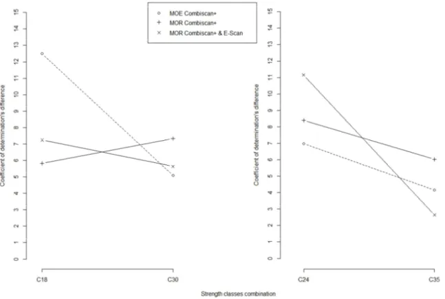
Figure 8 shows the improvement of the coefficient of determination on the whole batch of boards (for both bending and tension) for two combinations of strength classes. Note that the strength grading has been done with the destructive data; the whole batch of boards is divided into different batch that fulfill the requirements of the different grade described in the EN 338 (each sub-batch of boards meets the requirements in terms of density,
MOE and MOR). The gain observed is always positive but seems to decrease for the higher classes; this observation is more noticeable for the prediction of MOE.
3.4 Error induced by the grain angle linear variation hypothesis on the prediction of MOE and MOR
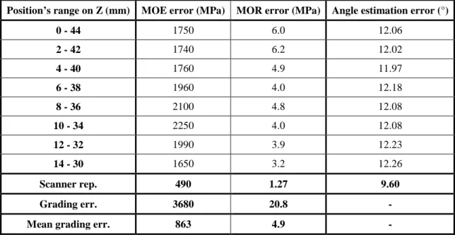
The grain angle estimation angle has been evaluated and compared to the scanner’s accuracy for this particular measurement. The estimation error, based on a 99% confidence interval is presented in Table 6 for each step of planning and at each resulting thickness. This error is on average 2° higher than the measurement accuracy and remains constant through the board’s thickness. The linear regression hypothesis can consequently be considered reasonable in clear wood areas.
The error induced in the mechanical properties by the grain angle linear variation hypothesis is shown Table 5, for each position’s range on Z for the 11 boards described above. These values can be compared to the scanner’s degree of repeatability (“Scanner rep.”), and its estimation error, i.e. the error between the corrected IPs and destructive tests results (“Grading err.”) expressed as well as a 99% confidence interval.
4
Discussions
Due to the high variability of timber in terms of mechanical properties, the numerical values of the results presented above cannot be guaranteed on another batch of boards. Indeed the fact that our batch of boards is composed of low and high quality timber, the presence of very high and very low values stretches the data cloud and gives better coefficient of determination. Nevertheless, the grain angle measurement should still permit an improvement for grading timber. However, the number of tested boards, native to various countries across Europe, is in accordance with EN 14081 (AFNOR, 2011) which contains standards requirements for grading machines certification. These results consequently highlight a stable and reproducible tendency. Sawmills should choose the right machine corresponding to their production and evaluate if buying more than one machine is financially viable, so the results analysis must take this parameters into account. Furthermore, adding the grain angle measurement to the Combiscan + is cheaper than buying an E-Scan. Concerning the comparison between grading performances with and without taking in account the slope of grain, it is clear that this information allows improvement of the optical scanner’s prediction accuracy for both MOE and MOR, in tension as well as in bending. In particular, taking into account the grain angle for the MOE prediction with the CombiScan+ allows to get closer to the E-Scan accuracy and permits the use of the CombiScan+ alone while keeping a reasonable accuracy on the MOE prediction. Adding the slope of grain information to the combination of the
E-Scan & CombiE-Scan+ does not permit a high improvement but this combination seems viable if both of MOE and MOR predictions are decisive for the strength grading due to the highest accuracy that can be obtained on these two parameters. It also appears that the projection angle brings more accuracy than the diving angle, despite the fact that, theoretically, both are of the same mechanical importance. The reason is probably that the projection angle measurement comes directly from laser light ellipses orientation, whereas diving angle is estimated from less accurate ellipses patterns statistics. Besides, it seems that estimation of the latter is dependent on the surface roughness, which induces additional uncertainty on the estimation of the spheroid eccentricity e0. Due to the equation 6 and 8, this uncertainty is highly prejudicial around 0°, i.e. in clear wood areas. Furthermore, the fact that the gain seems higher for lower class may be explained by their hypothetical higher nodosity and consequently the deviation of the grain angle around these knots.
The study of the grain angle variation between the top and bottom faces reveals that the measured error in terms of grain angle is the same order of magnitude as the scanner’s degree of repeatability, although around 2° above. It is important to note here that the scanner’s repeatability test has been performed on another batch of spruce boards. The fact that the angle estimation error remains stable regardless the position on Z axis can indicate two possibilities: either the 12° error corresponds to the scanner’s repeatability for this particular batch, or the validity of the linear variation hypothesis does not depend on the z position, and can therefore be extended on thicker boards. In both cases, it can be assumed that this hypothesis remains reasonable on clear wood areas. Its influence on the whole board grading, thus including knotty areas, shows that the error induced on MOE and MOR estimation is clearly above the scanner’s repeatability level, but remains under its grading error. An improvement in the grain angle modeling would likely reduce the MOR error, but would have a fewer importance in the MOE estimation. The fact that the MOR error due to this hypothesis increases with the board’s thickness, whereas MOE error does not seem to confirms this hypothesis. This can be explained by the fact that, contrary to the elastic modulus of a beam, the strength depends on the local mechanical properties near the area of the initial fracture. In other words, a single error in the estimation of slope of grain can greatly change the prediction of MOR, but will have a little effect on the MOE.
5
Conclusions
It is well known that knots are the predominant strength reducing defects of timber. Machines able to locally detect them and grade the boards accordingly already exist on the market, but the improvement potential in this field remains important. The grain angle is often seen as a strong candidate to enrich grading models due to its
high influence on clear wood mechanical properties. Yet, its impact on full boards strength grading had not been quantified.
The results of this study show that grain angle measurement, associated to the grading model presented above, can significantly improve the optical scanner’s performances as a strength grading machine. The main limitations on this field are the accuracy of the grain angle measurement, especially concerning the fibers diving angle, and the modeling of fibers angle across the board’s thickness. We saw that a linear variation model is acceptable, but could also be improved. The other way to improve the grading machines performances would consist in taking in account other types of singularities such as juvenile or compression wood.
6
Acknowledgements
The present project is supported by the National Research Fund, Luxembourg. LERMAB is supported by the French National Research Agency through the Laboratory of Excellence ARBRE (ANR-12- LABXARBRE-01).
7
References
AFNOR, 2009. NF EN 338, Bois de Structures - Classes de Résistance, 5 p.
AFNOR, 2010. NF EN 384, Bois de Structures - Détermination des valeurs caractéristiques des propriétés mécaniques et de la masse volumique, 11 p.
AFNOR, 2011. NF EN 14081, Structures en bois – Bois de structure à section rectangulaire classé pour sa résistance
AFNOR, 2012. NF EN 408, Structures en bois – Bois de structure et bois lamellé-collé – Détermination de certaines propriétés physiques et mécaniques
Baño V., Arriaga F., Soilán A., Guaita M. (2011). Prediction of bending load capacity of timber beams using a finite element method simulation of knots and grain deviation. Biosystems engineering, 109, 241-249
Brancheriau L. (2002). Expertise mécanique des sciages par analyse des vibrations dans le domaine acoustique, PhD thesis, Univ. Aix Marseille II, France, 278 p.
Brännström M., Manninen J. and Oja J. (2008). Predicting the strenght of sawn wood by tracheid laser scattering. BioResources 3: 437-451.
Guitard D. (1987). Mécanique du Matériau Bois et Composites, Cepadues, 238 p.
Hanhijärvi A., Ranta Maunus A., Turk G. (2005). Potential of strength grading of timber with combined measurement techniques. Report of the Combigrade project phase 1. VTT Publications568.
Hu C., Tanaka C. and Ohtani T. (2004). On-line determination of the grain angle using ellipse analysis of the laser light scattering pattern image. J. Wood Sci. 50: 321-326.
Kienle A., D’Andrea C., Foschum F., Taroni P. and Pifferi A. (2008). Light propagation in dry and wet softwood. Optics Express 16 n°13. 12 p.
Nyström J. (2003). Automatic measurement of fiber orientation in softwoods by using the tracheid effect. Computers and Electronics in Agriculture 41: 91-99.
Oh J.K., Shim K., Kim K.M. and Lee J.J. (2009). Quantification of knots in dimension lumber using a single-pass X-ray radiation. Journal of Wood Science 55: 264-272.
Pope D., Marcroft J. and Whale L. (2005). The effect of global slope of grain on the bending strength of scaffold boards. Holz als Roh- und Werkstoff 63: 321-326.
Roblot G., Coudegnat D., Bleron L. & Collet R. (2008). Evaluation of the visual stress grading standard on French Spruce (Picea excelsa) and Douglas-fir (Pseudotsuga menziesii) sawn timber. Ann. For. Sci. 65, n° 812, 4p.
Rohanovà A., Lagana R. & Babiak M., (2011). Comparison of non-destructive methods of quality estimation of the construction spruce wood grown in slovakia. 17th international nondestructive testing and evaluation of wood symposium, Hungary
Simonaho S.P. and Silvennoinen R. (2004). Light Diffraction from Wood Tissue. Optical Review 11: 308-311.
Simonaho S.P., Palviainen J., Tolonen Y. and Silvennoinen R. (2004). Determination of wood grain direction from laser light scattering pattern. Optics and Lasers in Engineering 41: 95-103.
Tredwell T. (1973). Visual Stress Grading of Timber, Explanation and practical interpretation of the visual grading elements of BS 4978:1973. Timber grades for structural uses, Timber Research and Development Association, 31p .
TABLES
Section (mm²) Number of samples
Bending 35x100 113 1017 45x110 58 45x150 177 50x150 253 60x175 243 75x220 173 Tension 45x110 58 356 35x210 125 45x150 58 45x195 115 Total : 1373
Table 1: Range of cross-sections and number of samples
Parameters Values
Image's acquisition Each board scanned five times Scanning direction Normal/End/Reverse/End+Reverse
Power of the X-Ray source 750/1050/1400/1800 Detection treshold of the ellipse 30/33/35/37/40
Table 2: Selected parameters to evaluate scanner's repeatability, underlined values are the defaults.
Min Mean Max StD CV (%) R2 ρ MOE MOR
ρ (kg.m-3) 294 432 634 49.93 12 ρ - 52% 27% B en d in g
MOE (MPa) 2840 11230 20560 2891 26 MOE - - 69%
MOR (MPa) 10.23 40.15 87.15 13.24 33 MOR - - -
ρ (kg.m-3) 301 393 529 35.88 9 ρ - 52% 24% T en si o n
MOE (MPa) 5790 10290 17940 2187 21 MOE - - 66%
MOR (MPa) 7 28.55 74.60 12.54 44 MOR - - -
Table 3 : Min, mean max values, standard deviations, coefficient of variation and coefficient of determination for different properties measured
Bending Tension
MOE MOR MOE MOR
E-Scan - 87% 57% 91% 58% CombiScan+ 0 65% 48% 73% 65% φ 73% 60% 78% 71% ψ 70% 55% 77% 71% θ 74% 61% 80% 74% CombiScan+ & E-Scan 0 87% 62% 91% 73% φ 87% 64% 91% 77% ψ 87% 61% 91% 74% θ 87% 63% 91% 78%
Table 4 : Strength grading R² coefficients between predicted and measured properties
Position’s range on Z (mm) MOE error (MPa) MOR error (MPa) Angle estimation error (°)
0 - 44 1750 6.0 12.06 2 - 42 1740 6.2 12.02 4 - 40 1760 4.9 11.97 6 - 38 1960 4.0 12.18 8 - 36 2100 4.8 12.08 10 - 34 2250 4.0 12.08 12 - 32 1990 3.9 12.23 14 - 30 1650 3.2 12.26 Scanner rep. 490 1.27 9.60 Grading err. 3680 20.8 -
Mean grading err. 863 4.9 -
FIGURES LEGENDS
Figure 1 – Local densities map obtained by X-Ray analysis.
Figure 2 – Relationship between θ, φ and ψ. The observed face is the z = 0 plane.
Figure 3 - Actual technology used in the scanner (top) and illustration of the different measured parameters (bottom).
Figure 4 – Four cases of grain angle observation and their effects on the elliptic pattern. Figure 5 – Grading process overview.
Figure 6 – Calculation of the parameters a and b (top) and comparison between density measured by X-Ray and manually measured (bottom).
Figure 7 – Comparison of predicted and tested values for MOE on the left and for MOR on the right for three different methods in tension.
Figure 8 - Difference of R2 between models with and without consideration of the slope of grain for two combinations of strength classes for both bending and tension.
FIGURES
Figure 1 – Local densities map obtained by X-Ray analysis.
Figure 2 – Relationship between θ, φ and ψ. The observed face is the z = 0 plane.
Figure 3 - Actual technology used in the scanner (top) and illustration of the different measured parameters (bottom).
Figure 4 – Four cases of grain angle observation and their effects on the elliptic pattern.
Figure 6 – Calculation of the parameters a and b (top) and comparison between density measured by X-Ray and manually measured (bottom).
Figure 7 – Comparison of predicted and tested values for MOE on the left and for MOR on the right for three different methods in tension.
Figure 8 - Difference of R2 between models with and without consideration of the slope of grain for two combinations of strength classes for both bending and tension.