Ravenna: Department of Economics, University of California – Santa Cruz, Institute of Applied Economics, HEC Montréal and CIRPÉE
I would like to thank Luca Benati, Thomas Cooley, Mark Gertler, Bart Hobijn, Oscar Jorda, Peter Ireland, Giorgio Primiceri, Francisco Ruge-Murcia, Paolo Surico and Carl Walsh for helpful discussion on earlier drafts of this project. Lorena Saiz Matute provided excellent research assistance.
Cahier de recherche/Working Paper 10-29
The Impact of Inflation Targeting : Testing the Good Luck Hypothesis
Federico Ravenna
Abstract:
Over the last twenty years the level and volatility of inflation decreased across industrial
countries. The inflation stabilization can be explained by a shift in monetary policy or by
a lucky period of low volatility in business cycle shocks. To test the “luck hypothesis” we
examine the inflation experience of Canada, one of the earliest and most successful
adopters of an inflation targeting monetary policy. We Kalman-filter the historical
structural shocks consistent with an estimated DSGE model. The estimated shocks are
used to build counterfactual histories. Ex-ante the model predicts inflation volatility to
more than halve under inflation targeting. But conditional on the shocks, we show that
the luck hypothesis can explain with a high probability Canada’s low inflation volatility
since the early 1990s. Any inflation stabilization induced by the shift in policy is
accounted for the most part by the impact on expectations. Counterfactuals built
neglecting expectations would prove the inflation targeting policy irrelevant.
Keywords: Business cycle shocks, Kalman filter, Credibility, Inflation targeting
1
Introduction
Over the last twenty years industrial countries have experienced a marked decline in the level and volatility of inflation, interest rates, and long term inflation expectations. The recent period of low and stable inflation can be attributed either to a change in the propagation mechanism of the economy -the most prominent explanation being a shift in -the management of monetary policy - or to a reduction in the volatility of exogenous shocks.
What are the reasons behind the observed change in inflation behaviour across industrial coun-tries? This paper examines the inflation performance of Canada, an early and successful adopter of an inflation targeting monetary policy since February 1991, and asks whether it can be explained by the ’luck hypothesis’. Accepting the luck hypothesis means that conditional on the exogenous shocks that hit the Canadian economy since 1991 the inflation time series would not have been significantly different under an alternative monetary policy. We focus on the impact of inflation targeting in reduc-ing inflation volatility, which dropped in Canada from 2.28 over the 1981-1990 decade to 0.51 over the following 1991-2000 decade, and to 0.48 over the 1991-2005 period (year-over-year core CPI inflation measured at monthly frequency, reported in Longworth, 2002, Murray, 2006). Our estimates show that the luck hypothesis cannot be rejected. At the same time, nearly all of the impact of inflation targeting on the behaviour of inflation was caused by the change in the private sector’s beliefs for monetary policy. The results are based on a methodology that builds upon, and expands on, a vast literature on constructing historical counterfactuals using restrictions from DGSE models.
The experience of inflation targeting countries is especially suitable to assess whether good luck or good policy can account for the observed change in inflation behaviour across industrial countries, since the monetary authority explicitly announced - and committed to - the inflation targeting policy. Countries adopting inflation targeting have experienced lower and more stable inflation, and a decline in the volatility of a wide range of other macroeconomic indicators. On the contrary, in the US case
the existence of a shift in monetary policy regime over the last 25 years is still widely debated. 1
Canada adopted inflation targets in 1991, aimed at stabilizing inflation around a long-term level of 2%. The change in policy happened at a time when inflation was feared to escalate again after the
1
While Boivin and Giannoni (2006), Cogley and Sargent (2005) and Clarida et al. (2000) provide evidence that US monetary policy did change in the 1980s, and affected the observed behaviour of inflation, the results in a number of papers do not support the claim of a shift in the systematic behaviour of US monetary policy, or the claim that it was responsible for the observed decline in real activity volatility (Ahmed, Levin and Wilson, 2004, Bernanke and Mihov, 1998, Canova and Gambetti, 2006, Justiniano and Primiceri, 2006, Primiceri, 2005, Sims and Zha, 2006, Stock and Watson, 2003).
significant reduction achieved in the 1982-84 period, following the economic boom at the end of the 1980s, an oil-price shock, and the introduction of a value added tax. A number of studies (Longworth, 2002, Ravenna, 2009) have documented that since 1991 there have been profound changes in the behaviour of inflation - beside its lower average level - including changes in its volatility, persistence, predictability, and in the slope of the Phillips curve. The average value of one measure of inflation uncertainty fell from 2.43 in 1981-1990 to 1.15 in 1991-2000, and the range of the forecast for long term inflation, a measure of dispersion in inflation expectations, fell from 6.55 to 2.91 across the two subsamples (Longoworth, 2002). An important objective of the inflation targeting policy is to reinforce the stability of the inflation process. The Bank of Canada itself documents that "the short run response of inflation to measures of excess demand and supply appears to have fallen" (Dodge,
2002). 2 Finding cross country evidence that inflation targeting improves macroeconomic performance
has been challenging (Ball and Sheridan, 2005, Cecchetti and Debelle, 2006, Goncalves and Carvalho, 2009, Levin, Natalucci and Piger, 2004), raising the possibility that the observed inflation stability was the result of good luck shared across industrial countries. Yet cross country evidence on the impact of inflation targeting may be hard to come by because aversion to inflation variability increased across most industrial countries since the 1980s (for cross country comparisons, see Bernanke, Laubach, Mishkin and Posen, 1999, Cecchetti and Ehrmann, 2002, Mishkin, 1999, Mishkin and Schmidt-Hebbel, 2002, Neumann and von Hagen, 2002, and Truman, 2003).
We investigate the impact of the shift in monetary policy by building counterfactual histories of the Canadian economy since the adoption of inflation targeting conditional on the earlier monetary policy and on a vector of shocks Kalman-filtered from data on ten aggregate variables. The shocks vector and the counterfactual history are constrained to be consistent with a maximum likelihood-estimated staggered wage and price adjustment DSGE model of the economy.
Contrary to counterfactuals built from VAR reduced-form models, as in Ahmed, Levin and Wilson (2004), Canova and Gambetti (2009), Primiceri (2005), Sims and Zha (2006), our approach allows for the policy change to affect the private sector’s expectations. Since a stated goal of inflation targeting central banks has been to change inflation expectations, the VAR reduced-form approach is likely to provide a distorted picture (see Benati and Surico, 2009). Our methodology is closer to the approach used by King and Rebelo (1998), Justiniano and Primiceri (2006), Rotemberg and Woodford (1998), and similar to the ’business cycle accounting’ in Chari, Kehoe and McGrattan (2007).
2Admittedly, core inflation standard deviation had been quite low in the second half of the 1980s, but it was even
As in the accounting approach, we take as a starting point a DSGE model, but we also allow for the possibility that the model may be too stylized to describe the data dynamics. Thus we introduce an additional vector of disturbances that identifies sources of fluctuations beyond the ones summarized in the DSGE model, and estimate the DSGE structural shocks with a Kalman filter. This same methodology is used by Christiano, Motto and Rostagno (2008), and is related to Ireland (2004) and Boivin and Giannoni (2006), and to the technique to estimate DSGE models in Sargent (1989). We provide a comparison of the results under three alternative methodologies. Our estimation shows that forcing the DSGE model to explain all the volatility in the data would overturn the result from the counterfactual exercise. Neglecting the policy impact on expectations would also bias the result from the counterfactual exercise.
We innovate relative to the Kalman filtering literature by showing two alternative ways to build counterfactuals so as to evaluate how much of the economy dynamics in the inflation targeting period is accounted for by the change in the path of the policy instrument (a shift in the actual policy) and by the announcement of an inflation target that is credible and affects expectations (a shift in the perceived policy)
Finally, we provide an explicit metric to evaluate the likelihood of the luck hypothesis. To test the luck hypothesis we ask what was the probability of observing the counterfactual inflation history conditional on the inflation targeting policy. In this way we can evaluate whether the counterfactual path would have been a more or less likely draw given the estimated variance of the shocks.
The main conclusions we reach are as follows.
With a high probability good luck can explain the low inflation volatility throughout the infla-tion targeting period in Canada. This result obtains despite model estimates implying the uncondiinfla-tional expected volatility of inflation to more than halve in the inflation targeting regime. We do not interpret the evidence for the luck hypothesis as implying that monetary policymaking is irrelevant. Inflation targeting simply may have not been put to test by inflationary shocks. But our result does support the good luck over good policy explanation, and - contrary to a vast literature on the impact of inflation targeting - implies that the shift in monetary policy cannot account for the historical improvement in inflation performance. While policies may be judged more or less desirable based on their uncondi-tional properties, the historical evaluation of their performance is only meaningful if conditioned on the business cycle shocks.
The counterfactuals show that inflation targeting affected the behaviour of inflation for the largest part through the impact on expectations. Monetary policy shocks are estimated to have
non-negligible variance, yet they contributed very little to inflation stabilization. Moreover, a monetary policy that did not affect private sector expectations but nevertheless stabilized inflation at its historical level would have lead to a severe and prolonged recession. This result supports the claim that changes in policy regime can dramatically affect the economy dynamics by altering private agents’ decision-making (Sargent, 1999), and the empirical observation that inflation targeting in Canada managed to de-couple inflation expectations from recently observed inflation rates (Dodge, 2002).
As for the methodological contribution, our result that alternative approaches to build counter-factuals can overturn the evaluation of the luck hypothesis illustrates the importance of allowing for a vector of non-structural disturbances when filtering the historical business cycle shocks. The Kalman filtering approach we adopt allows the data to choose what is the portion of business cycle volatility that the DSGE model can explain. Our methodology to assess the impact of a change in the path of the policy instrument separately from the impact of a change in the private sector expectation of policy can be applied to measure the announcement effect of any change in policymakers’ behaviour.
The paper is organized as follows. Section 2 compares alternative methods to build counterfac-tual histories and presents our empirical strategy. Section 3 presents the model. Section 4 explains the building of the Kalman-filtered counterfactual. Section 5 discusses the maximum likelihood estimation of the model and builds counterfactuals histories to evaluate the role of the policy rule, the role of policy shocks, and the role of credibility on Canadian inflation performance, and to assess the luck hypothesis. The implications of alternative methodologies are discussed. Section 6 concludes.
2
Counterfactual Histories to Evaluate the Impact of Policy Changes
A counterfactual history is defined by two components: a series of historical shocks εtand a
counterfac-tual law of motion. This section considers a baseline case to illustrate our empirical approach. Section 4 discusses the general case, and Appendix 7.3 provides the derivation of the equations in the following. Let the rational expectation equilibrium law of motion for a linearized DSGE model be given by the first order non-singular VAR process:
Yt= Γ1Yt−1+ Γ2εt (1)
where Yt = [yt, xt]0, yt is a vector of endogenous control variables, xt is a vector of endogenous state
variables, εt is vector of exogenous shocks randomly distributed. The VAR approach to generate a
(1) to build the historical shocks [εt]Tt=1. Couterfactuals are built by changing the coefficients in the row
of Γ1, Γ2 corresponding to the policy rule adopted, while expectations are assumed invariant to policy.
3 Benati and Surico (2009) have shown that the VAR approach can have low power in discriminating
between structural changes in the economy and changes in the exogenous shocks variance.
Our strategy is to derive the equilibrium law of motion (1) from estimation of a DSGE model,
and then use the DSGE reduced-form model to construct the historical shocks [εt]Tt=1. This approach
has been adopted by various authors, among which Arias, Hansen and Ohanian (2007), Benati and Mumtaz (2008), Justiniano and Primiceri (2006), King and Rebelo (1998), Rotemberg and Woodford
(1998), Stock and Watson (2003)4. Chari, Kehoe and McGrattan (2007) use a similar methodology,
although the ’business cycle accounting’ they propose identifies time-varying wedges in equilibrium decision-rules consistent with a whole family of models, rather than structural shocks from a uniquely identified model. Because this approach estimates the structural coefficients of the DSGE model, it is possible to build the counterfactual law of motion by solving the DSGE model conditional on the
alternative policy. Therefore, all the elements of Γ1, Γ2 are allowed to change, and expectations are
model-consistent.
An important drawback of this methodology is that by construction it requires a small set of structural shocks and the model internal propagation mechanism to explain all the volatility in the data. It is an accounting approach that does not allow for deviations from the DSGE model law of motion when building the model-consistent shocks vector. This requirement can be very taxing for the stylized models used in the DSGE literature. The Kalman filtering approach (Christiano, Motto
and Rostagno, 2008, Ireland, 2004) allows for the existence of an additional vector of disturbances wt
uncorrelated with εt. The vector wt identifies sources of fluctuations beyond the shocks included in
the DSGE model, which are given a structural interpretation. The law of motion for the observable variables is then:
Yt= Γ1Yt−1+ Γ2εt+ wt (2)
In essence eq. (2) augments the DSGE model so that there exists a residual variance in the data that the model is not called to explain in terms of movements of the structural shocks. This approach thus 3For applications of this approach, see Bernanke et al. (1999), Mishkin and Posen (1997), Canova and Gambetti
(2009), Sims and Zha (2006). It is possible to build VAR counterfactuals where expectations are policy-consistent, as in Ahmed, Levin and Wilson (2004) and Primiceri (2005). But in this case there is no assurance that the VAR counterfactual accounts exclusively for a change in the policy rule.
4These authors use the state-space representation of the equilibrium law of motion rather than the VAR representation.
The state-space representation does not require that the vector xtbe observable to obtain the historical series εt.Ravenna
allows for part of the observable variables’ variance to be explained by the vector wt when estimating
the model-consistent shocks vector, while it uses exclusively the DSGE model to build a counterfactual path with model-consistent expectations.
Empirical research using counterfactual histories to ascertain whether the change in the ob-served time-series of a macroeconomic aggregate must be ascribed to a change in exogenous shocks or behavioral parameters typically uses data before and after the observed change. We adopt a more parsimonious approach, and only use data after the adoption of inflation targeting in Canada. Thus we cannot discuss what was the cause of the observed change in inflation volatility before and after the inflation targeting policy adoption - whether, for example, the volatility of exogenous shocks did change across subsamples - but we can test whether the change in monetary policy was relevant or not for the behaviour of inflation volatility in the inflation targeting period. It may very well be that inflation targeting would have lowered inflation volatility in the earlier sample, or that the shocks from the earlier sample would have lead to high inflation volatility despite the switch to inflation targeting. These claims are distinct from the hypothesis we test, and are conditional on an estimated shocks’ vector that was never faced by the monetary authority in the inflation targeting period.
Our approach does not require estimation of the DSGE model over two subsamples - for the pre-inflation targeting period, only an estimate of the policy rule is needed . To impose as few constraints as possible on the data, we estimate the policy rule using a GMM estimator. The GMM estimator allows the use of a larger data set, which is useful since a number of time series used in the DSGE
model estimation post-1991 are only available starting in 1984.5
3
The General Equilibrium Model
The Canadian economy is modeled as a small open economy with nominal price rigidities, along the lines of the recent literature on monetary models of the international business cycle (see Bergin, 2003, Gali and Monacelli, 2005, Kollmann, 2001). The domestic (H) sector utilizes labor to produce a consumption-good basket that is both consumed by domestic households and exported to the foreign (F ) sector, in exchange for a foreign-produced consumption good.
A fraction of households and domestic firms set respectively nominal wages according to the Erceg, Henderson and Levin (1999) staggered contracts mechanism, and prices as in Calvo (1983). The
5
To obtain comparable estimates of the policy rule coefficients before and after the adoption of inflation tagerting, we estimate the policy rule with GMM over the two subsample, and estimate the DSGE model parameters given the inflation targeting policy rule estimates.
remaining fraction is assumed to follow a rule of thumb, so that price and wage setting is partially backward-looking. Households’ preferences have a habit-persistence specification. These three features improve the performance of sticky-price models, whose failure to generate plausible degrees of output and inflation persistence and to match the empirical correlation between real wages and output is well known (Fuhrer, 2000). Christiano, Eichenbaum and Evans (2005) and Rabanal and Rubio Ramirez (2005) provide evidence that nominal wage rigidity is at least as important as nominal price rigidity in accounting for US and Euro area business cycle fluctuations. Finally, the model allows for short-term incomplete pass-through from the foreign to the domestic price of imported goods.
3.1
Consumption Good Aggregates
Assume a continuum of infinitely lived households, indexed by j ∈ [0, 1]. Domestic households can
purchase a basket of differentiated home- and foreign-produced goods. The consumption aggregate Ct
combines the domestic (CH) and foreign (CF) goods basket in the same proportions as household j
would choose: Ctj = [(1 − γ)1ρ(Cj H,t) ρ−1 ρ + γ1ρ(Cj F,t) ρ−1 ρ ]ρ−1ρ (3)
where 0 ≤ γ ≤ 1 is the share of the foreign good and ρ > 0 is the elasticity of substitution between domestic and foreign goods. The domestic good H and the foreign good F are Dixit-Stiglitz aggregates defined over a continuum of differentiated goods indexed by i ∈ [0, 1] with elasticity of substitution
ϑ. Households allocate their expenditure optimally across goods. Pt, PH,t and PF,t indicate the price
indices for the aggregate, domestic and foreign good consumption basket.
3.2
Firms
The home production sector is made up of a continuum of firms indexed by i ∈ [0, 1]. Domestic firms produce goods by combining labor services supplied by households. Firms regard each household j’s
labor supply Ntj as an imperfect substitute for the labor offered by other households. A CES labor
aggregator Nt= (R01N jφφ
−1
t dj)
φ−1
φ combines households’ labor services in the same proportions as firms
would optimally choose. The wage index Wt= (
R1 0 W
j1−φ
t dj)
1
1−φgives the least expenditure that buys
a unit of the labor index. Firm i optimal demand for each type of labor j, conditional on the total
demand for labor services Nt(i), is equal to:
Ntj(i) = (W
j t
Wt
The total cost of the differentiated labor services hired by firm i isR01Ntj(i)Wtjdj = Nt(i)Wt. The firm
producing good i employs a CRS technology: Yt(i) = AtNt(i),where At is an aggregate productivity
shock. The firms’ cost minimization problem implies that when inputs quantities are chosen optimally
the real marginal cost M Ct is independent of the scale of production. We adopt the hybrid pricing
model in Gali and Gertler (1999). As in the time-dependent Calvo (1983) pricing model, in every
period t firms adjust their prices with probability (1 − θp). A fraction (1 − ωp) of the price resetting
firms update the price optimally, while a fraction ωp follows a backward-looking rule of thumb. The
problem of the firm optimally setting the price at time t consists of choosing PH,t(i) to maximize
Et ∞ X s=0 (θpβ)sΛt,t+s ∙ PH,t(i) PH,t+s YH,t+s(i) − M Ct+sN PH,t+s YH,t+s(i) ¸ (5) subject to YH,t+s(i) = ∙ PH,t(i) PH,t+s ¸−ϑ Ct+sW (6) M Ct+sN = PH,t+sM Ct+s = Wt+s M P Lt+s (7)
where M CN is the nominal marginal cost, M P L is the marginal product of labor. In (6), Y
H,t+s(i)
is the demand function for firm i output at time t + s, conditional on the price set s periods in
advance at time t, PH,t(i). Market clearing ensures that YH,t(i) = CtW(i) ≡ CH,t(i) + CH,t∗ (i) where
CH,t∗ (i) = (PH,t(i)
PH,t )
−ϑC∗
H,t is foreign demand for good i, CH,t∗ = γ∗Ct∗ is foreign demand for domestic
exports and Ct∗ is the exogenously given foreign aggregate demand for imports. Aggregate world
demand is defined as CtW ≡ CH,t+ CH,t∗ . The stochastic discount factor between t and t + s is βsΛt,t+s.
Backward looking firms update their price to the average level set in the most recent round of price
adjustment, Pt−1, adjusted for the lagged domestically-produced goods inflation rate πH,t−1 :
PH,tRT(i) = PH,t−1(1 + πH,t−1)
Conditional on the shocks vector at time t, the rule of thumb price PH,t+kRT (i) converges to the optimal
price as k → ∞. This hybrid model ensures that current inflation is determined partly by lagged and partly by expected inflation. At the same time, contrary to the indexation model assumed, for example, in Christiano et al. (2005), it does not constrain all firms to change prices every period.
3.3
Households
Households’ preferences are described by the instantaneous utility function:
Utj = ( [ln(Ctj− bCt−1j )]Dt− Ntj1+η 1 + η + ν Ã Mtj Pt !)
where Mt/Pt is real money balances, Nt is the amount of labor service supplied, Dt is an exogenous
preference shock that distorts the labor-leisure decision. Hall (1997) defines this shock as a shift in ”households’ choice between work in the market and time spent in non-market activities”. When b > 0 preferences are characterized by habit persistence. State-contingent claims ensure consumption levels are identical across households who supply different amounts of labor services. The aggregate consumption risk cannot be fully diversified, since on the international financial market the only asset traded is a riskless nominal bond. Households maximize the expected discounted utility flow:
Uj = E0 ∞ X t=0 βtUtj(Ctj, Ntj,M j t Pt , Dt)
subject to eq. (3) and the budget constraint:
PtCtj+ M j t + etvt∗Bt∗j+ +−→vt−→Bjt ≤ W j tN j t + M j t−1+ etBt−1∗j + Bt−1j + Πjt− τt (8)
where et is the nominal exchange rate, v∗t is the price of a zero-coupon riskless bond priced in foreign
currency, Bt∗ is the amount of foreign asset purchased, Wt is the wage rate, Πj is the share of profit
from the monopolistic firms rebated to the household, and τ is a lump sum government tax. Each
element of the row vector −→vt represents the price of an asset that will pay one unit of currency in a
particular state of nature in period t + 1. The corresponding element of−→Btrepresents the quantity of
such claims purchased by the household. Bt−1 indicates the value of the household portfolio of claims
against domestic residents given the current state of nature.
Households set the nominal wage Wj in contracts which can be renegotiated with probability
(1−θw). Of the households resetting the wage contract, a fraction (1−ωw) updates the wage optimally,
while a fraction ωw follows a backward-looking rule of thumb. Eq. (4) and the index of aggregate
employment Nt =
R1
0 Nt(i)di give household j0s downward sloping demand function for its type of
labor: Ntj = (W j t Wt )−φNt (9)
As in the staggered wage adjustment model of Erceg et al. (1999) any household j optimally resetting
the wage at time t maximizes its utility functional with respect to the nominal wage ˜Wtj, subject to
the sequence of budget constraints (eq. 8) and the labor demand function (eq. 9) at time t + s .
We assume the rule of thumb adopted by a fraction ωw of the wage-resetting households takes into
account the average nominal wage, the CPI inflation rate and the average contract duration 1−θ1
w, as in Rabanal (2001). Backward looking households update the wage to the average level prevalent across
all contracts at time t − 1, adjusted for the current inflation rate πt:
WtRTj = Wt−1(1 + πt)
1
1−θw (10)
For ωw → 0 the model converges to the Erceg et al. (1999) wage-updating mechanism. This
hy-brid model implies aggregate nominal wage inflation depends explicitly on current and expected CPI inflation through the indexing rule (10).
3.4
Import Sector
We model incomplete pass-through of imported goods prices by assuming that the foreign-produced good F is purchased by a continuum of monopolistically competitive firms in the import sector as an input for production (see Monacelli, 2005). Each firm z can costlessly differentiate the imported good
XF to produce a consumption good CF(z) using the production technology YF(z) = XF(z), where
XF(z) denotes the amount of input imported by firm z. The nominal marginal cost of producing one
unit of output is defined as M CN
F,t(z) = etPF,t∗ where PF,t∗ is the foreign-currency price of XF. The
domestic-currency price PF(z) is set following the Calvo (1983) pricing model with a probability of
price re-optimization equal to (1 − θF) . The producer faces an aggregate demand schedule given by:
YF,t(z) = ∙ PF,t(z) PF,t ¸− CF,t
where market clearing implies YF,t(z) = CF,t(z). This production structure generates deviations from
the law of one price in the short run, while asymptotically the pass-through from the price of the imported good to the price of the consumption basket F is complete.
3.5
Government Sector and Aggregate Shocks
The government budget is balanced in every period t. The central bank monetary policy is described
by the interest rate rule: ¡
1 + it ¢ (1 + iss) = ∙ Et µ Πt+1 ΠSS ¶¸ωπ ( YH,t YH,SS )ωy (11)
where ωπ, ωy ≥ 0 are the feedback coefficients to deviations of the expected gross CPI inflation rate
Πt+1 = PPt+1t and domestic output from their steady state values ΠSS, YH,SS. We assume the
policy-maker adjusts the interest rate only gradually to the target rate it:
(1 + it) =
£¡ 1 + it
¢¤(1−χ)
[(1 + it−1)]χεi,t (12)
where χ ∈ [0, 1) is the degree of smoothing and the exogenous shock εi,t represents non-systematic
movements in the monetary policy instrument. The logarithm of the exogenous preference shock Dt,
technology shock At, aggregate foreign demand Ct∗, and the world interest rate ˜ı∗t and imports’ price
inflation PF,t∗ /PF,t−1∗ follow a first order autoregressive stochastic process, with random innovation
εj,t ∼ N(0, σ2j). The exogenous policy shock εi,t is assumed to have no serial correlation. Market
clearing conditions and aggregate equilibrium conditions are in Appendix 7.6.
4
Counterfactual Histories: Methodology
Write the linearized DSGE model equilibrium law of motion as:
ξt+1 = F ξt+ vt+1 (13) qt = H 0 ξt (14) n+m×1ξ t = ⎡ ⎣ n×1ξ 1 t m×1ξ2 t ⎤ ⎦ = ⎡ ⎣ xt−1 zt ⎤ ⎦ (15) n+m×1v t = ⎡ ⎣ n×10 m×1εt ⎤ ⎦ (16) n+m×n+mF = ⎡ ⎣ n×nF 11 n×mF12 m×n0 m×mF22 ⎤ ⎦ (17) r×n+mH0 = h r×nH01 r×mH02 i (18)
E(vtv0t) = n+m×n+mQ = ⎡ ⎣ n×n0 n×m0 m×n0 m×mΣ ⎤ ⎦ (19) E(vtvτ0) = [0] f or τ 6= t (20)
qt is an r × 1 vector of observable variables, which may include elements of both the endogenous
state vector xt and control vector yt. εt is a multivariate Gaussian stochastic process with covariance
matrix Σ and unconditional expectation E(εt) = 0. Capital letters denote matrices. The index in the
upper-left corner indicates the size of a matrix.
The law of motion in eqs. (13), (14) can be inverted to obtain the vectors ξ1t and ξ2t conditional
on a vector of observable variables qt. Given an initial condition ξ0 and matrices F, H0 the state vector
ξt can be calculated from the recursion:
ξ1t = F11ξ1t−1+ F12ξ2t−1 (21)
ξ2t = (H02)−1[qt− H01ξ1t] (22)
For H02 to be invertible only m out of the r variables in the vector qt must be included. ξ2t is the
historical shocks vector consistent with the DSGE model and the observation vectors [q1...qt]. Eq.
(13) can be used to back out the corresponding series of innovations εt. We label this procedure the
’accounting approach’. Its mechanics imply that under the historical policy the model-simulated path
for the observables conditional on the historical vector ξ2t is identical to the data. Chari, Kehoe and
McGrattan (2007) use the accounting approach to measure how much of the business cycle fluctuations
can be explained by each shock during historical episodes6.
The accounting approach constrains the structural shocks to explain all of the variance observed in the data. We relax this assumption by assuming that the observable variables are described by the vector qto:
qto= qt+ wt (23)
where wt is an r × 1 Gaussian vector stochastic process with covariance matrix R:
E(wtwt0) = R ; E(wtw0τ) = [0] f or τ 6= t ; E(vtwτ0) = [0] ∀ τ (24)
6Chari, Kehoe and McGrattan’s (2007) ’business cycle accounting’ identifies time-varying wedges in the equilibrium
decision-rules, rather than structural shocks, since the covariance matrix Σ is not restricted to be diagonal. The authors show that a large class of models is equivalent to a prototype model with time-varying wedges.
In the econometric literature wt is assumed to represent a measurement error vector. It can be
in-terpreted as summarizing the volatility in qto which is not explained by the DSGE model. For the
system defined by eqs. (13), (14) and (23), and given the assumptions in equations (15) to (20), (24)
we define the linear projection of ξt+1 on the sample [qo1...qto] and a constant as the Kalman filtered
estimate ξt+1|t and Pt+1|t the associated mean squared error (MSE). The Kalman smoothed estimate
ξt|T ≡ ˆE(ξt|q1o...qTo) of the vector ξt is based on the full sample of observable variables, and Pt|T is the associated MSE.
A counterfactual history [q]Tt=1is built by simulating the model in eqs. (13) and (14) conditional
on a counterfactual law of motion F11, F12, H0and on the estimate [ξ2t|T]T
t=1. Because the model includes
the vector of disturbances wt, simulation of the historical equilibrium law of motion F, H0 conditional
on the filtered structural shocks in εtwill not generate the historical data series. Part of the variance in
the observable qto is accounted for by wt, while the vector εt (and the implied ξ2t vector) only explains
the variance of the unobservable qt. Therefore any counterfactual history qt by construction generates
a counterfactual path for qt rather than qto. The law of iterated projections implies that the Kalman
smoothed estimate qt|T ≡ ˆE(qt|qo1...qTo) is equal to H0ξt|T. The vector qt|T can be compared to the
counterfactual qt conditional on ξ2t+1|T, which is computed as:
ξt+1 ≡ ⎡ ⎣ ξ 1 t+1 ξ2t+1 ⎤ ⎦ = ⎡ ⎣ F 11 F12 0 I ⎤ ⎦ ⎡ ⎣ ξ 1 t ξ2t+1|T+ eξ2t+1 ⎤ ⎦ (25) qt = H0tξt (26)
where F11, F12, H0 describe the counterfactual law of motion and ξt describes the counterfactual path
of the state variables. For eξ2t = 0 ∀ t the system in eqs. (25) and (26) simulates the economy dynamics
when only the law of motion is changed. In some instances it is useful for some of the eξ2t components
to be nonzero in order to build counterfactual histories conditional on alternative shocks series. Note that by construction this method uses only the DSGE model in building a counterfactual history, since
all the variance in qt|T and qt is explained by the model structural shocks. The vector wt enters in the
5
The Impact of Inflation Targeting
The building of the Kalman-filter counterfactuals proceeds as follows. First we estimate the monetary policy rule coefficients over the inflation targeting sample and over the earlier 1971-1990 sample using a GMM estimator. Then we use the Kalman filter to evaluate the likelihood function of the model in eqs. (13), (14) and (23) conditional on the GMM estimates over the inflation targeting sample. The
maximum likelihood estimates are used to filter the historical shocks [ξ2t|T]Tt=1 and to compute
counter-factuals using eqs. (25) and (26) and the appropriate choice of F11, F12, H0. A detailed description of
the data set and estimation procedure is contained in Appendices 7.1 and 7.2.
5.1
Estimation
5.1.1 Monetary Policy Rule
Canadian monetary policy in the period before and after the adoption of inflation targeting is estimated on quarterly data using a two-stage GMM estimator with heteroschedasticity and autocorrelation
consistent covariance matrix. The orthogonality condition exploited in the GMM estimation is E[it−
(1 − χ)α − (1 − χ)ωππt+1 − (1 − χ)ωyyt− χit−1|ut] = 0 where α is a constant and ut is the set of
instruments. It is obtained by combining eqs. (11), (12) and taking a loglinear approximation around the steady state. The instruments set is similar to the one used by Clarida et al. (1998), and includes: four lags of the interest rate, inflation rate, money supply growth rate and three lags of the Hodrick-Prescott filtered output. Including lagged values of the real exchange rate among the regressors did not significantly modify the results.
The inflation targeting sample runs from 1992:1 to 2005:1. Inflation targeting was formally adopted in the first quarter of 1991, and the first target was set to reduce CPI inflation in the 1 to 3 percent range by the end of 1995, although inflation averaged 2% already in the first year. Before the announcement of specific inflation targets, the Bank of Canada had embarked in a three-year campaign to promote price stability as the long term objective of monetary policy, though it made little headway against the momentum in inflation expectations that had built up. In the fourth quarter of 1990
inflation was still at 4.2%. The pre-inflation targeting sample on which ωπ, ωy, χ, α are estimated
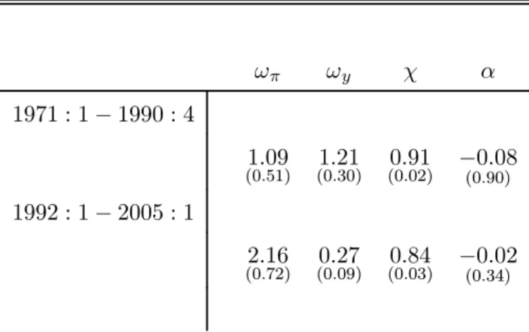
runs from 1971:1 (following the eight year period ending in 1970 when Canada pegged its exchange rate to the US dollar) to 1990:4. Table 1 reports the estimates, showing that in the inflation targeting period the weight on expected inflation increased from 1.09 to 2.16, while the weight on the HP-filtered output measure dropped from 1.21 to 0.27. The estimate of the coefficient χ on lagged interest rate
remained very high across subsamples. All estimated coefficients are significant at least at the 5% confidence level.
5.1.2 Maximum Likelihood Estimation
We estimate the small open economy model using a maximum likelihood estimator as in Bergin (2003) and Ireland (2004). The object of the estimation is the state-space representation of the loglinear approximation to the DSGE model law of motion, as specified in eqs. (13), (14) and (23). The
likelihood function for the sample [qot]Tt=1 can be constructed using the Kalman filter, and depends
nonlinearly on the structural parameters. The Sims (1999) algorithm is used to search for values of the DSGE model parameters and of the matrix R that will maximize the likelihood function.
The DSGE model parameters are estimated over the 1991:1 to 2007:2 sample using the observed data vector for 10 variables:
qto= [YH,t, πt, it, St, et/et−1, CH,t∗ , ˜ı∗t, ξt, Nt, M Ct]o
where the o superscript indicates that the observation available for variable xj,t is given by xoj,t= xj,t+
wj,t. The output variable YH,t is measured by the sum of constant-price consumption and net exports,
consistent with the model definition of output that includes only domestic and foreign consumption
of the home produced good: YH,t = CH,t+ CH,t∗ . Canadian real GDP over the same sample is about
20% less volatile, and shows a very similar pattern of correlations with the other macroeconomic
aggregates. The inflation measure πtis the seasonally adjusted CPI net of indirect taxes. The interest
rate it is the 3-month T-bill rate, although nearly identical results are obtained with the overnight
rate. The terms of trade series St= PF,t/PH,tis the ratio of the Laspeyres index for import and export
prices. Nominal exchange rate depreciation et/et−1 is obtained from the Canadian/US dollar exchange
rate (trade with the US accounts for about 80% of total Canadian international trade). The exports
series CH,t∗ is given by the Canadian constant-price export index for goods and services. The foreign
interest rate ˜ı∗
t is the US 3-month T-Bill quarterly yield. Nominal wage inflation ξt is measured by
the average hourly earnings for the non-farm sector, including government but excluding the defense
and not-for-profit sectors. The series for total labor hours Nt is built using employment and average
weekly hours of the same non-farm sector. The real marginal cost M Ct is obtained from the unit
labor cost series for the business sector discounted by the appropriate price deflator. All series are
and Hodrick-Prescott filtered.7
The covariance matrix R for the shocks vector:
wt= [wYH,t, wπt, wit, wSt, wet/et−1, wCH,t∗ , w˜ı∗t, wξt, wNt, wM Ct]
is assumed to be diagonal. Ireland (2004) suggests a more flexible specification, allowing for a VAR
structure of the wt components. We experimented with this specification, but the ML estimates of
the VAR coefficients and cross-correlations were for the large part not significant, while the robustness of the search algorithm to the initial starting value decreased considerably. The covariance matrix Σ of the structural shocks innovations is assumed diagonal, except for the submatrix describing the covariances for the foreign shocks Ct∗, ˜ı∗t and PF,t∗ /PF,t−1∗ . The non-zero correlation across these shocks allows the model to generate a richer dynamics for the foreign sector, and at the same time is a more parsimonious specification than a full blown VAR system.
The variance of the wtdisturbance for ˜ı∗t cannot be separately identified from the variance of the
shock itself, and we constrain the corresponding element in the R matrix to be zero. We also constrain
to zero the variance of the wtdisturbance for itwhich cannot be separately identified from the variance
of the policy shock εi,t. The parameters η and φ are not identified. To estimate η, the inverse of the
steady state labor supply elasticity, the value of the steady state wage markup φ/(φ − 1) is assumed equal to 10%, implying φ = 11. Amato and Laubach (1999) estimate a sticky price/sticky wage model of the US economy and find a value of φ equal to 8.5 with a standard deviation of 6.1. We use the model’s steady state restrictions to set prior to estimation some additional parameters for which the data contain only limited information. The quarterly discount factor β is set to 0.99, which implies a steady state real world interest rate of 4 percent. The foreign good share γ is equal to the steady state ratio between imports and domestic output, and is set to 0.35, the average Canadian import/output ratio over the inflation targeting sample. Finally, the elasticity of substitution between domestic goods ϑ is set equal to 6, so that the markup in a flexible-price steady state is 20% (Gali and Monacelli, 2005).
Parameter Estimates ML estimates and standard errors for 30 parameters are reported in Table
2. Most of the parameters are estimated with a low level of uncertainty, including the elements of
the covariance matrix R. The estimate of the standard deviations for the wt vector components is
7
We chose to filter also the series for M Ctsince it is characterized by a strong downward trend throughout the inflation
of the same order of magnitude as the volatility estimate for some of the structural shocks in ξ2t. This suggests there are important features in the data that the DSGE model propagation mechanism
cannot account for. The standard deviation of the preference shock innovation is σd= 5.68. This value
is large compared to the other disturbances, but it is not unusual for models with nominal rigidities to require volatile shocks to fit aggregate data. Rabanal and Rubio Ramirez (2005) estimation of a sticky price/sticky wage model on US data yields a standard deviation of the taste shock twice as large
(σd = 11.88). Del Negro et al. (2006) estimate a preference shock standard deviation of 40.54 within
a large-scale New Keynesian model of the US economy. Hall’s (1997) empirical decomposition shows that most of the volatility in U.S. labor hours can be attributed to a preference shift between market and non-market activities, and is consistent with the empirical evidence in Eichenbaum, Hansen and Singleton (1988) on the co-movements of real wages, consumption and work effort.
The estimates for the price and wage setting parameters deserve an extended comment. The
estimates for θw imply an average wage contract duration of five quarters, with about two thirds of
the contracts being reset at the optimal wage . The average length of wage settlements in Canada over the 1991-2000 period is 29.77 months (Longworth, 2002), but this figure does not include contracts in the non-unionized sector, and worker’s unionization in Canada has been declining. Additionally, the
estimate for θw implies a measure for the interval between wage adjustment, rather than the interval
between contract renegotiations.
The estimate for θF implies an average price duration for imported good of 3.75 quarters. The
estimate of the price setting probability θp for the domestic production sector implies an implausibly
long average price duration of 16 quarters. In addition, a fraction ωp close to 0.9 of the prices are
adjusted according to rule of thumb behaviour. When estimating DSGE model on aggregate US postwar
data, other authors have obtained estimates in the 0.85−0.9 range for θpand in the 0.82−0.96 range for
the degree of indexation to past prices among the non-reoptimizing firms (Rabanal and Rubio-Ramirez, 2005, Smets and Wouters, 2005). A comparison with the full-indexation price updating mechanism in Chistiano et al. (2005) is useful to illustrate the implications of the ML estimated parameters. These authors assume that a fraction of the firms can reset the price to the optimal level, while the remaining fraction indexes to lagged CPI inflation. Given the timing assumptions, the loglinear equilibrium condition for inflation is:
πH,t = γ∗bπH,t−1+ γf∗Et−1πH,t+1+(1 − βθp)(1 − θp
) (1 + β)θp
γ∗b = 1 1 + β ; γ ∗ f = β 1 + β
where lower case letters indicate log-deviations from the steady state. Since any plausible parameteri-zation for β implies a value close to 1 to be consistent with estimates of the steady state real interest
rate, the Christiano et al. (2005) inflation equation necessarily assigns nearly identical weights γ∗b and
γ∗f to lagged and expected inflation, and a weight whose value is close to 1/2. The Gali and Gertler
(1999) rule-of-thumb price resetting mechanism we adopt results in the loglinear equilibrium condition:
πH,t = γbπH,t−1+ γfEtπH,t+1+(1 − ω)(1 − θp)(1 − βθp ) Ψ mct (28) γb = ω Ψ ; γf = βθp Ψ ; Ψ = θp+ ω[1 − θp(1 − β)]
The estimates in table 2 imply γb = 0.49 and γf = 0.51, that is coefficients on lagged and expected
inflation that are virtually identical to the ones that appear in the price indexation model (27). There-fore both price updating mechanisms generate similar reduced form dynamics for inflation. But to be consistent with the reduced form favored by the data, both the rule of thumb model and the price indexation model imply an average price duration inconsistent with the microeconomic evidence, too long for the first one (16 quarters), too short for the second one (1 quarter). We interpret this result as evidence that neither of the two price resetting mechanism can be considered fully structural.
Likelihood Ratio Tests We use the likelihood ratio to compare the fit of the estimated model to
a state-space model where none of the DSGE restrictions is imposed. This is a strategy used by Bergin (2003) to evaluate the performance of the estimated model against an unrestricted model which takes the same reduced form, and therefore nests the DSGE model.
Estimation of the unrestricted model involves finding a parameterization for the matrices F, H, Q, R that maximizes the likelihood function. Since none of the DSGE model cross-equation restrictions is imposed, the unconstrained model is bound to have a higher likelihood than the con-strained DSGE model. The likelihood ratio test evaluates the statistical significance of the improvement in likelihood obtained by removing the DSGE model restrictions. The test accounts for the degrees of freedom, equal to the number of entries in F, H and in the lower triangular portion of the covariance matrices Q, R, minus the number of estimated parameters in the restricted model. Results are reported in table 3. The test cannot reject the DSGE model restrictions, the p-value of the null hypothesis being
equal to 0.23.
The result that the unconstrained model does not perform significantly better compared to the hybrid DSGE model is in part to be attributed to the degrees of freedom allowed by the additional
vector of disturbances wt. The relevance of the wt vector can be evaluated comparing the estimated
DSGE model to a model where the variance of (some components of) wtis set to zero. Since the model
has only six structural shocks, at least four components of wt must have non-zero variance to avoid
stochastic singularity when estimating the model over the 10-variables data set. Table 3 shows the likelihood ratio test result when the non-zero variance components of wt are [wSt, wet/et−1, wξt, wNt]. The zero-variance restrictions on the matrix R can be rejected at any significance level. Any other choice of zero-variance restriction results in an even lower likelihood.
The likelihood ratio can also be used to evaluate the role of nominal rigidities in the model performance. Table 3 provides the likelihood ratio for the restricted model where domestic wages and
prices are reset optimally in every period (the parameters θp, θw, ωp, ωw are restricted to be equal to
zero) and the benchmark hybrid model. The restrictions are rejected, implying that nominal rigidities play a statistically significant role in fitting the data. Finally, we test separately for the significance of the nominal rigidity in the foreign good import sector. This test is meant to discriminate between the
producer and consumer currency-pricing hypothesis for the imported good. A value of θF = 0 implies
instantaneous, complete pass-though of foreign price movements. This restriction can be rejected at any level of significance, as shown in the last line of table 3.
5.1.3 Structural Shocks Estimate
The Kalman-smoothed estimate of the structural shocks over the 1991:1-2007:2 sample is in figure 1,
together with ±1 root mean square error (RMSE) bands. The foreign interest rate shock ˜ı∗t has no
RMSE band since is included among the observables. We assume no prior information is available at time t = 0, and the recursion starts with ξ1|0 = E(ξ1) and P1|0 = E{[ξ1− E(ξ1)][ξ1− E(ξ1)]0}.
The technology disturbance is on average negative until 1994, then takes both negative and positive values throughout the remaining sample. This behaviour is not at odds with the strong Canadian output expansion in the 1990s. It is consistent with the Hodrick-Prescott filtered series for output used in the estimation, and with output gap estimates published by the Bank of Canada in its Monetary Policy Report, which imply an increase in both output and potential output in this period. Up to 1995 the data also imply a large and persistently negative preference shock, contributing to the severity of the recession in the early 1990s. The preference shock is mostly negative throughout the
1990s, possibly proxing for the fiscal consolidation during part of the decade. The monetary policy shock is small over all the sample. The estimates indicate that policy shocks were more volatile in the early years of inflation targeting, while in the 2000 to 2002 period the monetary authority set lower interest rates then warranted by the policy rule.
Figure 2 plots the historical data together with the smoothed estimate qt|T for the variables
YH,t, it, St, CH,t∗ 8. The ±1 RMSE error bands for qt|T are computed from M SEqt|T ≡ E{[qt− qt|T][qt− qt|T]0} = H0P
t|TH + R.
5.2
The Luck Hypothesis and the Cost of Inflation Targeting
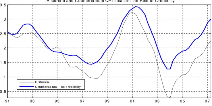
The first thought experiment compares the smoothed estimate of the historical annual CPI inflation
πt|T with the counterfactual path πtunder the hypothesis that inflation targeting had not been adopted
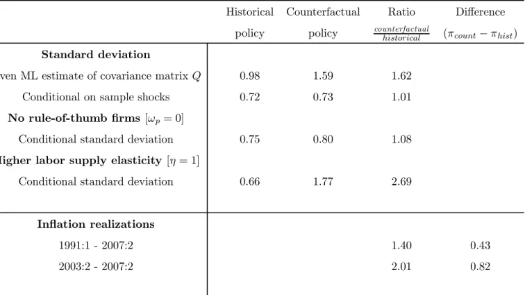
in 1991 (figure 3). It assumes ξ2t = ξ2t|T and that F11, F12, H0are computed conditional on the estimated pre-inflation targeting policy rule. We assume identical long-term inflation goals under the two regimes. Table 4 reports statistics to compare the two sample paths. The second row of table 4 shows that inflation targeting did not lower the realized volatility of inflation in the 1991 - 2007 period. What is remarkable is that while the volatility of inflation is virtually identical under the two policies conditional
on the Kalman-smoothed shocks vector ξ2t|T for the sample, the population volatility computed from
the ML estimate of the shocks’ covariance matrix bQ is more than 60% higher under the counterfactual
policy than in the inflation targeting regime. In other words, the historical shock vector was such that the policy rule had no impact on inflation volatility, even if ex-ante we would expect a change in inflation volatility.
Even if it did not affect significantly the volatility, the inflation targeting policy may still have had an important impact on the sample level of inflation, contributing to keeping it low. The last two rows of table 4 illustrate this point. Over the whole sample, inflation would have been on average 40% higher under the counterfactual policy. The level increase is even larger for the period following 2003. Since the average level of inflation is low, a 40% increase in inflation translates in an average inflation differential between the counterfactual and historical level of only 0.43 percentage points.
The Bank of Canada success in reducing inflation was associated by some critics with a high cost in terms of unemployment (Fortin, 1996). But it is by no means clear that the 10% unemployment rate reached in the early 1990s could be avoided using a different monetary policy (Mishkin and Posen,
8
If the estimate for qt is computed from the Kalman filtered series ξt|t−1, rather than the Kalman smoothed series
1997). In the same period world oil markets created inflationary pressures, while low commodity prices harmed Canadian exports. The output counterfactual (figure 3) shows the inflation targeting policy imposed a substantial cost in the period 1992-1994, when the extra output loss averaged slightly less than 0.5% of trend output per quarter.
Overall, it appears that monetary policy was largely irrelevant for inflation volatility, and helped to keep the inflation level lower after 2003. To assess the luck hypothesis, the appropriate question to ask is how likely a path of inflation as observed in the counterfactual history would have been under inflation targeting. To this end, we use the DSGE model to evaluate the probability of observing a given range of (smoothed) inflation values in any time t conditional on inflation targeting. Figure 3 plots the inflation unconditional 0.84 standard deviations bound above the mean computed from
simulating the DSGE model under inflation targeting. Since the vector qt has a multivariate normal
distribution, in the ergodic state 80% of the πt realizations will fall below the 0.84 standard deviations
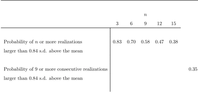
bound. The counterfactual inflation path lies above the 0.84 standard deviations bound in 15 periods over the sample. Yet in a long enough sample, inflation realizations as large as desired will occur even conditional on inflation targeting. Table 5 reports the results of a Monte Carlo exercise computing the probability of observing a given number n of inflation realizations above the 80% probability bound for the inflation targeting policy-maker over a sample as long as the 1991 to 2007 period. Would chance alone allow the economy to experience the performance of the non-inflation targeting policy - as many as 15 inflation observations above the 80% probability bound over 66 quarters? This event would not be unlikely at all: it would occur with a probability of 0.38. Even to generate the 9 consecutive inflation observation above the 0.84 standard deviations bound, as occurs in the counterfactual experiment between 2000:1 and 2002:1, the inflation-targeting central bank would not need much bad luck: such an event would be observed in 35% of the samples.
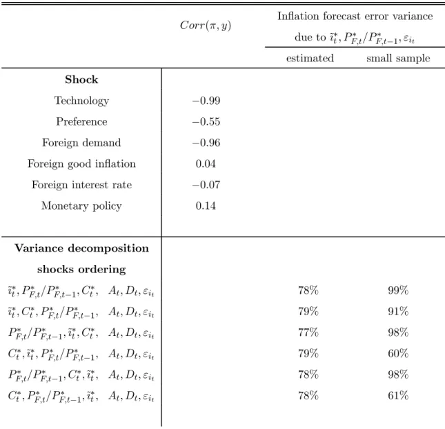
Since the shift to inflation targeting does generate a large decrease in the expected inflation volatility, what drives the result that in the sample the inflation behaviour is similar regardless of the monetary regime? After 1991 the estimated weights on the two variables entering the monetary reaction function, π and y, change in opposite directions. As a consequence, shocks that result in the model in a high negative correlation between inflation and output have the largest impact on the behaviour of policy, and ultimately on the counterfactual inflation time series. Table 6 shows the correlation between inflation and output in a hypothetical Canadian economy where all the business cycle volatility were generated by a single shock. Technology, preference and foreign demand shocks generate a very high negative correlation. If these shocks play a sufficiently large role in explaining the inflation volatility,
we would expect the counterfactual inflation time series to be strongly affected by the change in policy.
9 This is the case in the estimated model, where inflation volatility under the counterfactual policy is
more than 60% higher than in the inflation targeting regime when computed from the ML estimate of
the shocks’ covariance matrix Q. Using the ML estimate bQ, the forecast error variance explained by the
shocks ˜ı∗
t, PF,t∗ /PF,t−1∗ , εit - that do not generate a strong negative correlation for inflation and output - is between 77% and 79%. In the 1991:1 to 2007:2 sample, where the sample covariance matrix across the shocks is bQ =b T1ΣT
t=1bvtbv0t, the variance explained by the same shocks is for most orthogonalizations
above 90%.10 As a consequence, a change in the policy rule has a smaller than expected impact on the
inflation time series over the sample. Had, for example, the technology or preference shock played a larger role in explaining the inflation behaviour over the sample, the shift to inflation targeting would have resulted in a larger divergence between the historical and counterfactual inflation path.
Obviously the inflation behaviour results are also dependent on the parameter estimates. The
estimates for θp and ωp in the price-adjustment equation imply inflation is very inertial, and could
potentially limit the sensitivity of inflation to the policy rule. Table 4 shows that the large share of rule-of-thumb firms has only a small impact on the result. In an economy with no rule-of-thumb firms
(implying γb = 0 and γf = 0.99 in eq. 28) the counterfactual policy would have implied an increase in
inflation volatility of only 8%. Finally, it is legitimate to ask whether, given the Kalman-filtered shocks
vector ξ2t|T, the DSGE model is able to generate higher inflation volatility at all. This is indeed the
case. Table 4 includes the result from the counterfactual experiment conducted in an economy with a higher steady-state labor supply elasticity 1/η, increasing from 0.38 to 1. In this economy the sample
volatility would increase more than twofold relative to the inflation targeting policy case. 11
In summary, the estimation shows that the inflation path under the earlier monetary policy would have had a high likelihood of being generated also by an inflation targeting monetary policy. Chance alone resulted in a lower volatility of inflation over the period.
9This statement is not necessarily true in a DSGE model, since the correlation between inflation and output is
endoge-nous to the choice of policy. For the estimated model though the statement is accurate.
1 0
Since the estimation imposes overidentifying restrictions, the ML estimate eQcan differ from the covariance matrix of the sample shocks 1
TΣ T
t=1evtevt0. Note that since the covariance matrix is not diagonal, the fraction of inflation variance
attributable to each innovation depends on their order of preference. We assume foreign shocks are exogenous from Canada’s point of view, while Canadian shocks do not affect the rest of the world. The ordering of the domestic shocks does not alter the outcome of the variance decomposition exercise, and these results are not reported.
1 1
This result is provided to show that there exist model parameterizations which can imply a large impact of policy on inflation volatility conditional on the estimated sample shocks vector. It does not imply that the result on the impact of inflation targeting is extremely sensitive to the estimated parameters, since for different parameter estimates the Kalman-smoothed shocks vector would be different as well.
5.3
The Impact of Policy Shocks
The second counterfactual examines the impact of policy shocks in Canada by simulating an economy conditional on the inflation targeting policy but setting to zero the monetary policy disturbance (figure
4). The counterfactual assumes F11 = F11, F12 = F12, H0 = H0. We set the jth component of the
vector eξ2t, corresponding to the policy shock εi,t, equal to −ξ2
j
t|T so that ξ 2j
t = 0 ∀ t. The vector composed
of all the elements of ξ2t except the jth one, ξ2−j
t , is unchanged and equal to ξ2
−j
t|T .
The impact of policy shocks on inflation is limited over the sample, of the order of a quarter of a percentage point. Unexpected movements in monetary policy played a more important role in output dynamics. By lowering the interest rate level, they contributed to keeping output above trend over the 2002-2005 period. The improvement in output is as high as 1%. The counterfactuals show that the non-systematic component of monetary policy did not carry any weight for the poor output performance in the early 1990s.
5.4
The Impact of Credibility
Central banks adopting inflation targeting frameworks consider the achieved macroeconomic stability, at least in part, a result of the increased credibility of the policy commitment to inflation stabilization. Some authors (see Kuttner and Posen, 1999) argue instead that the adoption of inflation targeting simply indicates the central bank’s shift towards a greater conservatism with respect to the inflation goal, with increased credibility and transparency playing a minor role for the policy’s outcome.
The third counterfactual evaluates the role of the inflation targeting credibility in Canadian’s inflation performance since 1991 by building a history under the assumption that the shift in monetary
policy occurred but was not believed by the private sector (figure 5). It assumes ξ2t = ξ2t|T. The
matrices F11, F12, H0 are built under the hypothesis that the monetary authority adjusts interest rates
according to the estimated post-1991 inflation targeting policy (F11= F11, F12= F12, H0= H0), while
the private sector expectation eEtps[st+1] of any variable stis conditioned on the belief the central bank
adopts the policy rule estimated for the earlier period. Thus, while the actual policy changes relative to the pre-inflation targeting period, the perceived policy used to form the private sector’s expectation is unchanged. Effectively, the private sector interprets as non-systematic movements in the interest
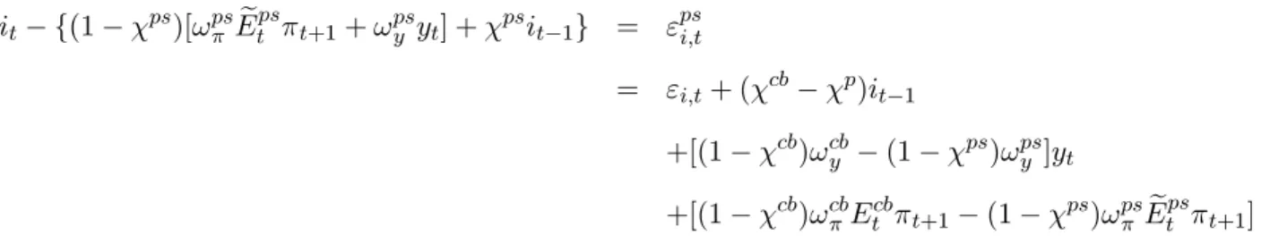
the true and believed policy rule: it− {(1 − χps)[ωpsπ Ee ps t πt+1+ ωpsy yt] + χpsit−1} = εpsi,t = εi,t+ (χcb− χp)it−1 +[(1 − χcb)ωcby − (1 − χps)ωpsy ]yt +[(1 − χcb)ωcbπEtcbπt+1− (1 − χps)ωpsπ Ee ps t πt+1]
where the index ps indicates the private sector believes, the index cb indicates the true value of a parameter in the central bank policy rule, and we assume the central bank’s expectation of inflation is
model-consistent: Etcbπt+1 = Etπt+1. Appendix 7.4 describes the equilibrium concept adopted to solve
the DSGE model when the private sector holds incorrect believes.
Figure 5 shows that despite the monetary authority increased aggressiveness towards inflation, a non-credible policy would achieve an inflation path very close to the one under the assumption inflation targeting had not been introduced at all (shown in figure 3), that is, under a less inflation-averse, but fully credible policy. By and large, the experiment shows that whatever change in inflation dynamics occurred over the inflation targeting period must be attributed to the change in the perceived policy. At the same time, the non-credible inflation targeting regime would not lead to as large a stabilization of output as the credible non-inflation targeting regime. The counterfactual shows that conditional on the shocks vector the largest part of the change in inflation dynamics after 1991 originated from the expectation channel: the private sector adjusting its behaviour given the belief that the central bank’s stance against inflation has become more aggressive.
To measure the gain from the expectation channel, we build a fourth counterfactual assuming the monetary authority still follows the inflation targeting policy without being believed by the private sector - but at each time t adjusts the nominal interest rate to bring inflation to its historical level
(figure 5). The counterfactual assumes the same matrices F11, F12, H0 as in the previous exercise while
eξ2tj is computed to ensure πt = πt. Appendix 7.5 provides the recursion to build the appropriate ξ
2j
t .
The counterfactual history describes an economy where the central bank achieves the given historical inflation path by actually changing the path of the interest rate through surprise policy interventions, rather than relying on its commitment to a policy rule to adjust the interest rate in response to the state of the economy.
Figure 5 shows the implied path of output. After 1996, output decreases persistently and dra-matically. In the counterfactual, when faced with inflationary shocks the monetary authority raises
interest rates and forces the economy into a severe recession to be able to achieve the inflation target path. Firms’ expect policy to be more accommodative towards inflation than it really is, and the incor-rect believes would lead firms to set persistently higher prices, ceteris paribus. The central bank reacts with unexpected increases in the nominal interest rate, that translate in real interest rate increases, to curb demand and the firms’ inflationary behaviour. Because only 6% of the prices are updated in every period, incorrect believes are very persistent in the economy, and result in a prolonged recession. The distance between the historical and counterfactual output represents the gain from cred-ibility: the extra movement in output relative to the one a credible central bank, achieving the same inflation rate, would have experienced. Ex-ante, the distance can be positive or negative, depending on the combination of shocks hitting the economy. Given the Kalman-smoothed shocks, it leads to a prolonged recession in the sample.
5.5
Alternative Methods to Build Counterfactuals
Figure 6 compares the baseline Kalman filtering method to two alternative methodologies to build a counterfactual inflation series conditional on the pre-inflation targeting policy. The top panel plots the
result from an exercise closer to the accounting approach. The shocks vector ξ2t|T is Kalman-filtered
using the DSGE model estimates in table 2 but assuming the only non-zero variance components of wt
are [wSt, wet/et−1, wξt, wNt]. This assumption allows using the same 10 data series to filter shocks as in the benchmark model. This fifth counterfactual is then obtained from the recursion in eqs. (21) and
(22) assuming F11, F12, H0 are built conditional on the estimated pre-inflation targeting policy rule.
The accounting method implies a shocks vector ξ2t with a larger variance, and this in turn returns a
counterfactual path for inflation which is much more volatile than the counterfactual smoothed estimate of inflation in figure 3. By construction, the Kalman filter methodology returns a more conservative
counterfactual path since a larger portion of the data volatility is explained by the vector wt. At the
same time, since the volatility of the unobserved component wπt is constrained to 0 in this exercise, the
counterfactual path must be compared to the observed historical path πo
t - which has a comparatively
higher variance than the smoothed estimate πt. Nevertheless, the accounting method would imply a
very substantial impact of the monetary policy shift on inflation dynamics. Over the whole sample, inflation volatility would increase by 59% relative to the historical volatility. The full-fledged Kalman-smoothed counterfactual implied an increase of only 1%.
The bottom panel of figure 6 still relies on the DSGE model, but shows a counterfactual