Computation of quasi-periodic localised vibrations in nonlinear cyclic and symmetric structures using harmonic balance methods

Science Arts & Métiers (SAM)

is an open access repository that collects the work of Arts et Métiers Institute of

Technology researchers and makes it freely available over the web where possible.

This is an author-deposited version published in:

https://sam.ensam.eu

Handle ID: .

http://hdl.handle.net/10985/16780

To cite this version :

Filipe FONTANELA, Aurélien GROLET, Loïc SALLES, Norbert HOFFMANN - Computation of

quasi-periodic localised vibrations in nonlinear cyclic and symmetric structures using harmonic

balance methods - Journal of Sound and Vibration - Vol. 438, p.54-65 - 2019

Any correspondence concerning this service should be sent to the repository

Computation of quasi-periodic localised vibrations in nonlinear

cyclic and symmetric structures using harmonic balance

methods

F. Fontanela

a,∗

_{, A. Grolet}

b

_{, L. Salles}

a

_{, N. Hoffmann}

a,c a_{Department of Mechanical Engineering, Imperial College London, Exhibition Road, SW7 2AZ, London, UK} b_{Department of Mechanical Engineering, Arts et Métiers ParisTech, 8 Boulevard Louis XIV, 59000, Lille, France} c_{Department of Mechanical Engineering, Hamburg University of Technology, 21073, Hamburg, Germany}

a r t i c l e i n f o

Article history: Received 29 May 2018 Revised 29 August 2018 Accepted 2 September 2018 Available online 10 September 2018 Handling Editor: Erasmo Carrera

In this paper we develop a fully numerical approach to compute quasi-periodic vibrations bifurcating from nonlinear periodic states in cyclic and symmetric structures. The focus is on localised oscillations arising from modulationally unstable travelling waves induced by strong external excitations. The computational strategy is based on the periodic and quasi-periodic harmonic balance methods together with an arc-length continuation scheme. Due to the pres-ence of multiple localised states, a new method to switch from periodic to quasi-periodic states is proposed. The algorithm is applied to two different minimal models for bladed disks vibrating in large amplitudes regimes. In the first case, each sector of the bladed disk is mod-elled by a single degree of freedom, while in the second application a second degree of free-dom is included to account for the disk inertia. In both cases the algorithm has identified and tracked multiple quasi-periodic localised states travelling around the structure in the form of dissipative solitons.

© 2018 Elsevier Ltd. All rights reserved.

1. Introduction

The emergence of localised vibrations in cyclic and symmetric structures is an important phenomenon due to potential problems induced by high cycle fatigue. Mechanical components with cyclic symmetry are very common in the aerospace industry, where e.g. bladed disks of aircraft engines [1], space antennas [2] and reflectors [3] are usually composed of ideally identical substructures assembled in a cyclic and symmetric configuration. In the linear framework localised vibrations arise due to the lack of symmetry induced e.g. by manufacturing variability or wear. This topic is well-known in the aerospace industry as a mistuning problem, and studies have mainly focused on effective modelling techniques [4,5], experimental characterisation together with model identification [6,7], and even the use of intentional mistuning to reduce the level of vibrations in real applications [8,9].

In real applications, structures may deviate from the linear behaviour e.g. due to frictional interfaces, large displacements, or fluid-structure interaction [1,10–13]. In the presence of nonlinearities the emergence of localised vibrations might go much beyond mistuning. It is well-known, for example, that even perfect cyclic and symmetric structures can localise vibrations in the nonlinear regime due to the dependence of mode shapes on amplitude, and also due to bifurcations [14–20]. Moreover, the effect of inhomogeneities when a system vibrates in the nonlinear regime is a challenging research field, and the role played by

nonlinearity in an inhomogeneous mechanical system experiencing energy localisation is an active topic [21,22].

This paper introduces a fully numerical approach to compute quasi-periodic states bifurcating from periodic vibrations due to nonlinearities. The focus is on localised states resulting from the emergence of modulation instability for travelling wave excitations in cyclic and symmetric structures. This investigation has been motivated by recent findings in Refs. [23,24], in which the authors show that localised states in the form of solitons bifurcate from travelling wave responses. The previous findings have been computed using an asymptotic method applied to a very idealised minimal model, and more flexible methods are required for the case of more complex and more realistic applications. The fully numerical approach proposed in this paper relies on harmonic balance methods (HBMs) for the computation of periodic and quasi-periodic vibrations. Moreover, due to the presence of several coexistent localised states, a method to switch from periodic to quasi-periodic branches near bifurcation points is introduced. The numerical approach is applied to two different minimal models: (1) a bladed disk with one degree of freedom per sector; and (2) a bladed disk with two degrees of freedom per sector. The computed results show that, in both cases, strong localised states are possible due to nonlinear envelope dynamics.

The paper is organized as follows. In Sec.2the fundamentals of the HBM is introduced, including a new technique to switch from periodic to quasi-periodic branches. Section3focuses on the investigation of two minimal models, and quasi-periodic localised solutions are computed using the approach described in Sec.2. Finally, Sec.4describes the main conclusions and suggests directions for future investigations.

2. The harmonic balance method

We investigate nonlinear dynamical systems mathematically described by

Mx

̈

(t) +Cx

̇

(t) +Kx(t) +f_nl(x(t)) =f_ext(t)

,

(1) where M, C, and K are the n× n mass, damping, and stiffness matrices, respectively, whilex

̈

(t),x

̇

(t), and x(t)represent the corresponding acceleration, velocity, and displacement vectors. In Eq.(1), f_ext(t)is the vector of external excitations, while the vector fnl(x)models the displacement dependent nonlinear forces.

We assume that the system in Eq.(1)is vibrating under periodic or quasi-periodic1 _{regimes. Therefore, x(t)is expanded in a} two-frequencies quasi-periodic Fourier series as

x(t) =a0,0+ h1 ∑ k1=−h1 h2 ∑ k2=−h2 ak1,k2cos ( k1

𝜔

1t+k2

𝜔

2t ) +bk1,k2sin ( k1

𝜔

1t+k2

𝜔

2t )

.

(2)

In Eq(2), h1and h2are the numbers of retained harmonics for the frequencies

𝜔

1and

𝜔

2, respectively, a0,0is the vector of static

displacements, while ak1,k2and bk1,k2are the vectors representing the Fourier coefficients. It is important to note that when h1 or h₂is null the quasi-periodic expansion in Eq.(2)recovers the standard periodic HBM (see e.g. Refs. [10,25,26]). Moreover, the quasi-periodic expansion is only valid when the two frequencies

𝜔

1and

𝜔

2are incommensurable, otherwise

𝜔

2can be written

as a harmonic of

𝜔

1and, consequently, x(t)is in the periodic regime (see e.g. Ref. [27]).

In the following we introduce a hyper-time domain with two independent variables

𝜏

₁ =

𝜔

1t and

𝜏

2 =

𝜔

2t. The scalar

product between two quasi-periodic functions f₁(

𝜏

₁

, 𝜏

₂)and f₂(

𝜏

₁

, 𝜏

₂)in hyper-time domain is defined as

<

f₁(

𝜏

1

, 𝜏

2)

,

f2(

𝜏

1

, 𝜏

2)

>

= ∫ 2𝜋 0 ∫ 2𝜋 0 f₁(

𝜏

1

, 𝜏

2)f2(

𝜏

1

, 𝜏

2)d

𝜏

1d

𝜏

2

.

(3)

The aim of the HBM is to transform the set of nonlinear differential equations in Eq.(1)into a system of nonlinear algebraic equations. This system is obtained after substituting Eq.(2)into Eq.(1), and finally projecting the resulting equation onto the trigonometric basis using Eq.(3). This process leads to

L(

𝜔

₁

, 𝜔

₂)z+g_nl(z) −g_ext=0

,

(4)

where L(

𝜔

₁

, 𝜔

₂)is the matrix representing the linear dynamics, z is the vector of unknown Fourier coefficients in Eq.(2), and 0 is the null vector. The matrix L(

𝜔

1

, 𝜔

2)is algebraically represented as [27–29]

L(

𝜔

1

, 𝜔

2) = ⎡ ⎢ ⎢ ⎢ ⎢ ⎢ ⎣ L0,0 0 … 0 0 L−h1,−h2 _{… 0} ⋮ ⋮ ⋱ ⋮ 0 0 … Lh1,h2 ⎤ ⎥ ⎥ ⎥ ⎥ ⎥ ⎦

,

(5)

where the inner matrices L0,0_{and L}k1,k2_are L0,0=K

,

Lk1,k2₌ [ K− (k1

𝜔

1+k2

𝜔

2)2M (k1

𝜔

1+k2

𝜔

2)C −(k₁

𝜔

₁+k₂

𝜔

₂)C K− (k₁

𝜔

₁+k₂

𝜔

₂)2M ]

.

(6)

In Eq.(4), gnl(z)and gextare the vectors projecting fnl(x(t))and fext(t)into the frequency domain, respectively. Usually, gnl(z)

is not directly computed since displacement dependent nonlinear forces are, most of the times, defined in the time domain. Therefore, an alternating frequency-time (AFT) domain technique based on the hyper-time concept [27,28,30], as depicted in

Fig. 1, is implemented. In order to illustrate this approach, suppose that the set of coefficients a00, ak1,k2and bk1,k2 in Eq.(2) are given. Therefore, the displacement field x(

𝜏

1

, 𝜏

2)and the corresponding nonlinear forces fnl(x(

𝜏

1

, 𝜏

2))define surfaces in

hyper-time domain. Finally, one can compute the Fourier coefficients of the nonlinear forces g_nl(z)using the scalar product in Eq.(3). However, in practice, g_nl(z)is obtained directly using a two-dimensional fast Fourier transform (2D-FFT). Similarly, the transformation from frequency to time domain can be implemented by means of an inverse 2D-FFT.

2.1. Harmonic selection

The number of harmonics defined by k₁ and k₂in Eq.(2)can be drastically reduced. Without any additional information regarding the nonlinear forces f_nl(x), the vector of unknowns z can be reduced to roughly half of its original dimension due to the symmetry properties (odd/even) of the harmonic functions. In the literature, several different techniques have been suggested to decrease even more the dimension of z and, consequently, the computational efforts [27,31]. In this paper we are interested in localised vibrations induced by strong travelling wave responses. It is well-known in the literature that localised solutions bifurcate from travelling wave states due to modulation instability [32–35]. In this case, any general physical coordinate xn(t)

can be written as

x_n(t) =

𝜓

(

𝜔

₂t)f_cw(

𝜔

₁t)

,

(7)

where

𝜓

(

𝜔

2t)is the modulating (or envelope) function dependent on

𝜔

2 only, and fcw(

𝜔

1t)is the carrier wave. One should

note that in the case of a carrier wave with no static component the spectrum of x_n(t), i.e. its frequency contain, cannot depend on

𝜔

2only. Therefore, the harmonics referred to k1=1 can be removed from the solution basis.Fig. 2displays two examples

of retained harmonics using the full basis and the reduced one. In Panel (a), for h₁=h₂=4, the number of retained harmonics reduces from 41, using the full harmonic expansion, to 36, using the modulation instability property. The reduction is more efficient when h2

≫

h1, as in Panel (b). In this case, for h2=7 and h1=1, the number of retained harmonics reduces from 23,

using the full harmonic basis, to 15, when solutions localise due to modulation instability. 2.2. Stability of periodic solutions

Stability of periodic solutions is addressed using Floquet theory. Thus, a small perturbation h(t)is added to an already known periodic solution x_p(t), and linear stability of x_p(t)is computed based on the evolution of h(t). In this case, three different configurations are possible: (1) if h(t)increases in time xp(t)is unstable; (2) if h(t)decreases over time then xp(t)is stable;

and (3) if h(t)is constant then the system is marginally stable and a nonlinear stability analysis is required. It is possible to demonstrate (see e.g. Ref. [36]) that the linear stability of x_p(t)can be computed from the so-called monodromy matrix𝚽. The most straightforward way to compute𝚽consists in time integrating the linearised system with periodic coefficients

̇

y(t) =By(t)

,

(8) where y(t) = {x(t)x

̇

(t)}T, and B= ⎡ ⎢ ⎢ ⎣ 0 I M−1_(K+

𝜕

fnl

𝜕

x ∣x=xp) M −1_C ⎤ ⎥ ⎥ ⎦

.

(9)

This integration is carried out over one period T using 2n linearly independent initial conditions. For simplicity, the ith initial condition is usually assumed as yi(0) = {0

,

0

,

0

,

…

,

1

,

…

,

0

,

0

,

0}T, where all terms of yi(0)are null except the ith one which has

the unity value. The final configuration of each ith solution, y_i(T), is grouped in a matrix𝚽as

𝚽 =[y₁(T)

,

…

,

y_i(T)

,

…

,

y_2n(T)]

.

(10)

The three possible scenarios about the stability of x_pare given by the eigenvalues

𝜌

_iof𝚽: (1) if max(|

𝜌

_i|)

<

1, the system is linearly stable; if max(|

𝜌

_i|)

>

1, the system is linearly unstable; and in the special case (3) when max(|

𝜌

_i|) =1, the system is marginally stable. In this paper, we are interested in unstable Floquet multipliers

𝜌

iwith imaginary parts different than zero

(Im(

𝜌

_i)≠0). In this case, the system experiences a Neimark-Sacker (NS) bifurcation, and a branch of quasi-periodic solutions detaches from periodic states.

2.3. Numerical continuation

In the case of quasi-periodic oscillations arising due to NS bifurcations the second frequency

𝜔

₂has to be treated as an unknown. This unknown can be added to the algebraic system by means of a phase condition. Physically, this phase condition pins down the envelope function by removing the intrinsic rotating symmetry of the problem. Mathematically, this constraint

Fig. 1. Hyper-time approach to compute the Fourier coefficients for the nonlinear forces. The fist line is associated with the hyper-time representation, while the second line illustrates the corresponding results in frequency domain (modulus of the 2D-FFT). Here we have chosen a displacement x(t) =cos(t) +cos(√2t) +cos(t+√2t) =

cos(𝜏1) +cos(𝜏2) +cos(𝜏1+𝜏2).

Fig. 2. Complete harmonics sampling (blue circle) and the modulation instability reduction (red cross). Panel (a) shows the results for h1=h2=4, while Panel (b) shows the harmonic basis for h1=1 and h2=7. (For interpretation of the references to colour in this figure legend, the reader is referred to the Web version of this article.)

can be included in Eq.(1)by setting one of the sinusoidal terms for the harmonic k₁=1 and k₂=1 as equal to zero. Therefore the new nonlinear algebraic system, with

𝜔

2as un unknown, is written as

( 0 0 ) = ( L(

𝜔

1

, 𝜔

2)z+gnl(z) −gext ai_1,1 ) (11)

Fig. 3. Strategy to switch from periodic to quasi-periodic branches. In the first step, the NS bifurcation is identified from the Floquet multipliers. In the second step the unstable mode is used as initial conditions for Eq.(8)and the growth rate from the computed response is removed. The final result is added to the corresponding periodic regime, in the third step, and the final configuration in frequency domain is used as an initial guess for the solution of Eq.(11).

where ai_1,1states the k1 = k2=1 cosine term for the ith degree of freedom. One should note that the harmonics k1=k2=1 and

the cosine term (instead of the sine term) have been chosen arbitrarily. In general, any non-zero quasi-periodic sine or cosine harmonic for any ith degree of freedom can be chosen as a phase condition.

In order to follow the solutions of Eq.(11), a numerical continuation scheme based on a tangent predictor and an arc-length corrector is implemented. The tangent prediction uses the Jacobian of Eq.(11), at a solution point, to estimate the next solution (see e.g. Ref. [37]). The arc-length corrector equation

0= ∥Z₀−Z(

𝜔

1

, 𝜔

2)∥2−s2

,

(12)

is added to the problem, where Z₀ is an already known previous solution and s is the step length. After adding Eq.(12)to the algebraic system in Eq.(11), the Fourier coefficients ak1,k2 and bk1,k2 as well as the frequencies

𝜔

1and

𝜔

2are treated as unknowns in the minimisation problem. This continuation scheme allows the periodic and the quasi-periodic HBM approaches to follow turning points (see e.g. Ref. [37]).

2.4. Branch switching

In this subsection we develop a strategy to switch from a periodic to a quasi-periodic branch. The most straightforward way to change from a periodic to a quasi-periodic branch uses results obtained from time integration [31,38]. In this case, solutions from unstable periodic regimes are used as initial conditions for a time-marching algorithm, and the system jumps to the quasi-periodic branch naturally. This approach works well if there is only one stable quasi-periodic solution within the analysed regime, and for unstable periodic states. In more complicated cases, when e.g. several quasi-periodic states coexist, it is difficult to guarantee that initial conditions from the unstable periodic state will lead the time integration scheme to the required quasi-periodic solution.

The new approach developed in this subsection does not require any stability condition for the quasi-periodic response, and also works for systems with several coexistent stable quasi-periodic solutions. Overall, the main idea is to use information from the monodromy matrix𝚽, evaluated at an unstable periodic solution, to generate an initial guess for the nonlinear algebraic problem in Eq.(11). The steps required are illustrated inFig. 3. Firstly, a Floquet analysis is carried out for the periodic solutions. It is well-known from the linear stability analysis that, close to the bifurcation point, perturbations h(t)increase exponentially with growth rate

𝜇

= 𝜔1

2𝜋Re{ln(

𝜌

i)} and pulsate with frequency

𝜔

2=

𝜔1

2𝜋Im{ln(

𝜌

i)}, where

𝜌

iis the corresponding unstable Floquet

multiplier. Therefore, this value of

𝜔

₂is assumed as an initial guess for the algebraic system in Eq.(11).

The second step consists in time integrating the tangent system in Eq.(8)using the real part of the corresponding unstable eigenvector of the monodromy matrix𝚽as an initial condition. Since the system is unstable with respect to this perturbation, the initial condition will increase exponentially in time with growth rate

𝜇

, as shown inFig. 3. The exponential part is then removed from the response, and the final configuration is a quasi-periodic signal with frequencies

𝜔

₁and

𝜔

₂. It is expected that nearby the NS bifurcation point perturbations will behave similarly to this linear approximation.

The final step uses information from the periodic state. This solution, which coexists with the quasi-periodic regime, is added to the previously calculated perturbation. The final state consists of a periodic state with a small quasi-periodic perturbation on top. The spectrum of this configuration is then used as an initial guess for the algebraic system in Eq.(11).

Fig. 4. Minimal model for the bladed disk with a single degree of freedom per sector.

It should be noted that the presented approach has two free parameters. The first one is the perturbation amplitude. Since initial conditions for Eq.(8)uses the unstable eigenvector of𝚽, these initial conditions may assume any arbitrary amplitudes values. The second free parameter is the value of

𝜔

1itself or, in other words, the distance from the computed solution to the

actual NS bifurcation point. We have observed, in the simulations of Sec.3, that far from the bifurcation point or with large perturbations amplitudes, the nonlinear algebraic problem has experienced convergence problems. On the other hand, when the system is solved very close to the bifurcation point, or with relatively small perturbations amplitudes, the algebraic system may converge to the undesired periodic regime. The compromise between these two parameters has been chosen empirically in the present investigation.

3. Numerical application

We apply the methodology described in Sec.2to compute quasi-periodic localised solutions bifurcating from nonlinear trav-elling waves in cyclic and symmetric systems. We then define

𝜔

_ias the ith linear natural frequency, and

𝜙

_ias the corresponding mode shape. Due to the cyclic symmetry, it is well-known that most of the eigenvalues come in pairs of

𝜔

_2iand

𝜔

_2i+1having the same values (degenerated eigenvalue), while the corresponding eigenvectors

𝜙

_2iand

𝜙

_2i+1are just shifted in space. Using the linear mode shapes of the cyclic structure, a travelling wave force f_tw(t), also known as an engine order excitation, can be defined as

f_tw(t) =

𝜙

2icos(

𝜔

Ft) +

𝜙

2i+1sin(

𝜔

Ft)

,

(13)

where

𝜔

F is the force frequency. The external excitation has just one harmonic, and the values of

𝜙

iand

𝜙

i+1are directly

applied as the Fourier coefficients within the HBM implementation. Moreover, the travelling wave in Eq.(13)can be seen as the superposition of two standing waves,

𝜙

_2iand

𝜙

_2i+1, in which the time evolution is with appropriately chosen phases.

In the following we study two different minimal models for bladed disks vibrating in nonlinear travelling wave regimes. Firstly, a physical system composed of a cyclic and symmetric chain of Duffing oscillators is assumed as a physical model for a bladed-disk operating in large displacements. A similar system has been already investigated in Refs. [23,24], where it has been shown that solitons bifurcate from unstable travelling wave responses. The second example introduces a more complicated minimal model composed of two degrees of freedom per sector. In this case, travelling waves with zero and one nodal circles are possible. In both cases several coexistent quasi-periodic states may branch off in the form of localised solutions.

3.1. Bladed disk with a single degree of freedom per sector

The system under investigation is depicted inFig. 4. It consists of Ns=24 masses m=1 kg, connected to each other by linear

springs k_c=1 N/m, and attached to the ground by linear springs k_l=1 N/m and viscous dampers c=0.01 Ns/m. Each mass is also connected to the ground by cubic springs k_nl=0.1 N/m3_{and subjected to external forces f}

n. This minimal model with geometric

nonlinearities can, for example, be obtained when the Von Karman theory is applied to a system of clamped beams or plates that are cyclically connected to each other by massless springs [10,39]. The N_sequations of motion for the system inFig. 4are written as

m

̈

x_n+cx

̇

_n+k_lx_n−k_c(x_n−1+x_n+1−2x_n) +k_nlx3_n=f_n

,

(14)

where x₁=x_N

s+1due to the cyclic symmetry.

In the following analysis the external force is assumed as an eighth engine order. For low excitation amplitudes, the system vibrates in an almost linear regime, and the frequency response functions (FRFs) show stable solutions only. For stronger forces the system looses stability due to NS bifurcations, and quasi-periodic solutions detach from the periodic branch.Fig. 5displays a typical result calculated for a travelling wave with force amplitude of 0.025 N. The plane wave solutions have been calculated with the periodic HBM assuming a series expansion with three harmonics (h₁=3). InFig. 5, solid black lines identify stable travelling waves, while the black dashed line represents unstable solutions. The plane wave FRF shows the usual stiffening effect, as expected due to the cubic springs. However, no periodic bi-stability is observed. In fact, homogeneous states loose stability

Fig. 5. FRF calculated from the HBM implementation, where the horizontal axis displays the external force frequency and the vertical one identifies the maximum vibration amplitude. The four insets display the spatial envelope function in four different configurations.

due to NS bifurcations before the first turning point (around 2.00 rad/s), and recover stability again only after the second turning point (around 2.02 rad/s). Inside the unstable periodic regime, two quasi-periodic branches detach from plane waves. The first NS bifurcation, computed from the Floquet analysis, is identified with the blue line inFig. 5. The branch is followed with the quasi-periodic HBM assuming one harmonic for the carrier wave (h1=1), and five harmonics for the envelope function (h2=5).

The quasi-periodic branch detaches from plane waves as weakly localised solutions but internally changes its configuration along the branch to a strongly localised dissipative soliton. This feature is highlighted by the envelope functions plotted in the insets inFig. 5. Moreover, around 2.01 rad/s another pair of unstable Floquet multipliers is computed, leading to the second branch of localised solutions identified by the red line inFig. 5. These solutions are calculated with the quasi-periodic HBM assuming h₁=1 and h₂=5. The branch comprises, again, localised states moving around the structure in the form of dissipative solitons.

Panels (a) and (c) ofFig. 6display the amplitude of each harmonic, for a specific degree of freedom, and for two solutions in the two different quasi-periodic branches of 5. These solutions show that sidebands components, equivalent to h₁=1 and h2= ±1, dominate the quasi-periodic dynamics. This is a typical feature of localised states emerging via modulation instability,

and it has been extensively investigated within the nonlinear Schrödinger equation framework [40–42]. Panels (b) and (d) show, in dashed red lines, the same solutions but in time domain. The curves show, as discussed before, localised humps preserving their shapes while they move around the system. The same graphs also identify, in black solid lines, the corresponding results computed from time-integration. The comparison between the quasi-periodic HBM and the time marching results are in very good agreement.

3.2. Bladed disk with two degrees of freedom per sector

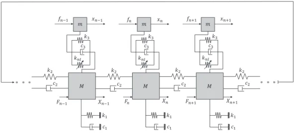
The physical model inFig. 7displays the bladed disk with two degrees of freedom per sector under investigation. In this case, the N_s=24 sectors are described by two degrees of freedom: (1) the masses M=1 kg refer to the disk inertia; and (2) m=0.3 kg models the blade masses. Each mass M is also connected to the ground by linear springs and viscous dampers k₁=1 N/m and c1=0.005 Ns/m, respectively, while the interaction between each sector is given by k2=1 N/m and c2=0.005 Ns/m. The

con-nection between the blade and the disc is given by the linear springs and dampers k₃=1 N/m and c₃=0.005 Ns/m, while the cubic spring k_nl=0.1 N/m3_{models the stiffening effect induced by large deformations. The set of equations for the 2N}

sdegrees

of freedom are written as

mx

̈

n+c3(x

̇

n−X

̇

n) +k3(xn−Xn) +knl(xn−Xn)3=fn (15)

MX

̈

n−c2(X

̇

n+1+X

̇

n−1−2X

̇

n) −c3(x

̇

n−X

̇

n) +c1X

̇

n−k2(Xn+1+Xn−1−2Xn) −k3(xn−Xn) +k1Xn−knl(xn−Xn)3=Fn

(16) Minimal models similar to the one inFig. 7are often used in the literature for the investigation of bladed disk vibrations [16,43]. Firstly, we compute the system responses due to travelling wave forces of eighth engine order and zero nodal circles. In this case, the blades and the disc are vibrating in phase, and nonlinearities are triggered by the difference between the two

Fig. 6. HBM results for two quasi-periodic solutions. Panel (a) displays the amplitude of each harmonic, for a specific degree of freedom, in the first quasi-periodic branch of Fig. 5. Panel (b) shows the comparison of HBM results with time marching (TM). Panels (c) and (d) show the same quantities of Panels (a) and (b), but for a solution within the second quasi-periodic branch ofFig. 5.

Fig. 7. Minimal for the bladed disk with two degrees of freedom per sector.

amplitudes. For low excitation forces, as expected, the system behaves similarly to the underlying linear model and solutions are always stable. However, for stronger excitations, the system looses stability and experiences NS bifurcations as in the previous example of Sub. 3.1.Fig. 8displays a typical result, obtained assuming an external force with amplitude of 0.01 N. The results have been calculated assuming h₁=3 for periodic solutions, while h₁=1 and h₂=5 for the quasi-periodic responses. In this case, again, no periodic bi-stability is observed, and two NS bifurcations are identified. The first quasi-periodic branch, identified by the blue line inFig. 8, shows a solution branching off from plane waves and internally changing its configuration to a strongly localised response with one hump before merging to the travelling waves again. The second quasi-periodic branch, in red, shows similar features ofFig. 5. In this case, again, localised solutions with two humps detach from plane waves and merge back to periodic solutions.

The results obtained from the quasi-periodic HBM approach are compared to time integration inFig. 9. Panel (c) shows an example for the first quasi-periodic branch inFig. 8, while Panel (f) illustrates the same quantities calculated from a solution in the second branch. In this case, as discussed before, each sector has the two degrees of freedom moving in phase. The results in time domain show humps of localised solutions moving around the structure preserving their shapes. The envelope function which modulates the disk and the blades have similar shapes, although they experience different amplitudes. This feature can

Fig. 8. Maximum blade displacement for a system with two degrees of freedom per sector. The results have been calculated assuming a travelling wave force with zero nodal circles and eight nodal diameters. The black lines show stable periodic solutions, and the black dashed line represents unstable ones. The blue and red lines are quasi-period solutions detaching from the branch of travelling waves. The insets show the spatial envelope function in four different configurations for the blade (blue and red lines) and the disk (black lines). (For interpretation of the references to colour in this figure legend, the reader is referred to the Web version of this article.)

Fig. 9. Responses for the two different quasi-periodic configurations inFig. 8. Panels (c) and (f) display the comparison of time marching (TM) results, with black solid lines showing time integration responses and red dashed lines identifying HBM results. Panels (a) and (d) show the blade spectra, while Panels (b) and (e) display the same quantities for the disk. (For interpretation of the references to colour in this figure legend, the reader is referred to the Web version of this article.)

be confirmed from Panels (a) and (d), which display the spectrum for a blade, and Panels (b) and (e), which illustrate the same quantities for the corresponding disk displacement. The spectra for the blade and the disk are essentially the same, differing only in amplitudes. These findings can be confirmed from the results in the four insets inFig. 8.

Finally, we investigate the system responses due to travelling wave forces of eighth engine order and one nodal circle. Physi-cally, the disk and the blades vibrate out-of-phase within this regime. The overall behaviour is similar to the previous examples, in which branches of localised solutions bifurcate from travelling waves when modulation instability is triggered.Fig. 10 dis-plays a typical result obtained for an external excitation with amplitude of 0.016 N. The periodic solution has been calculated assuming h₁=3, while the quasi-periodic branches have been computed assuming h₁=1 and h₂=7. Within this configuration, solutions are more damped than in the previous case, inFig. 8, since dampers c₃dissipate more energy. Moreover, nonlinear-ities play the role in lower amplitude regimes due to the out-of-phase motion, and localised solutions branch off for lower

Fig. 10. Maximum blade displacement for a system with two degrees of freedom per sector. The results have been calculated assuming a travelling wave force with one nodal circle and eight nodal diameters. The black lines show stable periodic solutions, and the black dashed line represents the unstable one. The blue and red lines are quasi-period solutions detaching from the planes waves. The insets show the spatial configuration in four different branches for the blade (blue, green, red, and purple bars) and the disk (black bar). (For interpretation of the references to colour in this figure legend, the reader is referred to the Web version of this article.)

Fig. 11. Responses for two different quasi-periodic configurations inFig. 10. Panels (c) and (f) display the comparison of time marching (TM) results, with black solid lines showing blade displacements and blue solid lines referring to the corresponding disk results, with the HBM implementation, in red dashed lines. Panels (a) and (d) show the blade spectra, while Panels (b) and (e) display the same quantities for the disk. (For interpretation of the references to colour in this figure legend, the reader is referred to the Web version of this article.)

displacement regimes. InFig. 10, three branches of quasi-periodic states detach from travelling waves. The first branch, in blue, resembles a dissipative soliton with three humps moving around the structure. However, the other two branches, in red and green, show more complicated patterns, and the modulating functions have more irregular shapes.

The previous HBM solutions are compared to time integration in Panels (c) and (f) ofFig. 11. The two displayed results are obtained from initial conditions in the first (blue) and in the third (green) branches inFig. 10. In both cases localisation arises due to modulation of travelling waves. In Panel (c), a regular hump moves around the structure preserving its shape. In Panel (f), the envelope function which modulates the travelling waves has a more irregular form, discussed before. Although this envelope function has an irregular shape, the final configuration still consists of a quasi-periodic motion with two incommensurable frequencies. The comparison between time integration and the quasi-periodic HBM shows good agreement. Panels (a) and (d)

inFig. 11display the spectra for the blade responses, while Panels (c) and (e) inFig. 11show the same quantities for the disc. The amplitude spectra for the blade and the disk are, again, very similar, although the graphs do not show any information about the differences in phase.

4. Conclusions and outlook

In this paper we have employed the periodic and quasi-periodic HBMs to compute nonlinear localised vibrations in cyclic and symmetric structures. The investigation has been focused on models experiencing nonlinearities induced by strong engine order excitations. The strategy has been applied to two different minimal models: (1) a chain of linearly coupled Duffing oscillators; and (2) a more complicated bladed disk model with two degrees of freedom per sector. In both cases multiple quasi-periodic coexistent states may exist, and a new strategy to track these several quasi-periodic states have been introduced. The results computed in this paper corroborate previous findings, showing that cyclic and symmetric structures subjected to large travelling wave forces may localise vibrations due to envelope dynamics.

The present paper has studied localised vibrations arising due to smooth nonlinearities. However, bladed disks of aircraft engines are often subject to friction and impact induced e.g. by root joint, underplatform dampers, shrouds and damper wires. Therefore, future investigations will also have to deal with localised vibrations involving non-smooth nonlinearities. More work also needs to be done on model accuracy. Thus, reduced-order models from fully nonlinear finite elements will also be addressed.

Acknowledgements

The first author is funded by the Brazilian National Council for the Development of Science and Technology (CNPq) under the grant 01339/2015-3.

References

[1] M. Krack, L. Salles, F. Thouverez, Vibration prediction of bladed disks coupled by friction joints, Arch. Comput. Meth. Eng. (2016) 1–48,https://doi.org/10. 1007/s11831-016-9183-2.

[2] O.O. Bendiksen, Mode localization phenomena in large space structures, AIAA J. 25 (9) (1987) 1241–1248,https://doi.org/10.2514/3.9773.

[3] O.O. Bendiksen, P.J. Cornwell, Localization of vibrations in large space reflectors, AIAA J. 27 (2) (1989) 219–226,https://doi.org/10.2514/3.10084,http://arc. aiaa.org/doi/10.2514/3.10084.

[4] M. Castanier, C. Pierre, Modeling and analysis of mistuned bladed disk vibration: current status and emerging directions, J. Propul. Power 22 (2) (2006) 384–396.

[5] P. Vargiu, C. Firrone, S. Zucca, M. Gola, A reduced order model based on sector mistuning for the dynamic analysis of mistuned bladed disks, Int. J. Mech. Sci. 53 (8) (2011) 639–646,https://doi.org/10.1016/j.ijmecsci.2011.05.010.

[6] J. Judge, C. Pierre, O. Mehmed, Experimental investigation of mode localization and forced response amplitude magnification for a mistuned bladed disk, J. Eng. Gas Turbines Power 123 (4) (2001) 940,https://doi.org/10.1115/1.1377872.

[7] D. Laxalde, F. Thouverez, J.J. Sinou, J.P. Lombard, S. Baumhauer, Mistuning identification and model updating of an industrial blisk, Int. J. Rotating Mach. (2007),https://doi.org/10.1155/2007/17289.

[8] M.P. Castanier, C. Pierre, Using intentional mistuning in the design of turbomachinery rotors, AIAA J. 40 (10) (2002) 2077–2086,https://doi.org/10.2514/3. 15298.

[9] C. Martel, J.J. Sánchez-Álvarez, Intentional mistuning effect in the forced response of rotors with aerodynamic damping, J. Sound Vib. 433 (2018) 212–229,

https://doi.org/10.1016/j.jsv.2018.07.020.

[10] A. Grolet, F. Thouverez, Free and forced vibration analysis of a nonlinear system with cyclic symmetry: application to a simplified model, J. Sound Vib. 331 (12) (2012) 2911–2928,https://doi.org/10.1016/j.jsv.2012.02.008.

[11] N. Akhmediev, E. Kulagin, Generation of periodic trains of picoseconld pulses in an optical fiber: exact solutions, Sov. Phys. Usp. 1 (April 1985) (1986) 894–899.

[12] A.C. Luo, Toward Analytical Chaos in Nonlinear Systems, John Wiley & Sons, 2014.

[13] L. Pesaresi, L. Salles, A. Jones, J. Green, C. Schwingshackl, Modelling the nonlinear behaviour of an underplatform damper test rig for turbine applications, Mech. Syst. Signal Process. 85 (2017) 662–679,https://doi.org/10.1016/j.ymssp.2016.09.007.

[14] A.F. Vakakis, C. Cetinkaya, Mode localization in a class of multidegree-of-freedom nonlinear systems with cyclic symmetry∗_{, SIAM J. Appl. Math. 53 (1)} (1993) 265–282,https://doi.org/10.1137/0153016.

[15] M. Sato, B.E. Hubbard, A.J. Sievers, Colloquium: nonlinear energy localization and its manipulation in micromechanical oscillator arrays, Rev. Mod. Phys. 78 (1) (2006) 137–157,https://doi.org/10.1103/RevModPhys.78.137.

[16] F. Georgiades, M. Peeters, G. Kerschen, J.C. Golinval, M. Ruzzene, Modal analysis of a nonlinear periodic structure with cyclic symmetry, AIAA J. 47 (4) (2009) 1014–1025,https://doi.org/10.2514/1.40461.

[17] N. Boechler, G. Theocharis, S. Job, P.G. Kevrekidis, M.A. Porter, C. Daraio, Discrete breathers in one-dimensional diatomic granular crystals, Phys. Rev. Lett. 104 (24) (2010) 244302,https://doi.org/10.1103/PhysRevLett.104.244302arXiv:1009.0885.

[18] A. Grolet, F. Thouverez, Computing multiple periodic solutions of nonlinear vibration problems using the harmonic balance method and Groebner bases, Mech. Syst. Signal Process. 52–53 (1) (2015) 529–547,https://doi.org/10.1016/j.ymssp.2014.07.015.

[19] A. Papangelo, A. Grolet, L. Salles, N. Hoffmann, M. Ciavarella, Snaking bifurcations in a self-excited oscillator chain with cyclic symmetry, Commun. Non-linear Sci. Numer. Simulat. 44 (2017) 108–119,https://doi.org/10.1016/j.cnsns.2016.08.004.

[20] A. Papangelo, N. Hoffmann, A. Grolet, M. Stender, M. Ciavarella, Multiple spatially localized dynamical states in friction-excited oscillator chains, J. Sound Vib. 417 (2018) 56–64,https://doi.org/10.1016/j.jsv.2017.11.056.

[21] M.V. Ivanchenko, T.V. Laptyeva, S. Flach, Anderson localization or nonlinear waves: a matter of probability, Phys. Rev. Lett. 107 (24) (2011) 1–4,https:// doi.org/10.1103/PhysRevLett.107.240602.

[22] T. Ikeda, Y. Harata, K. Nishimura, Intrinsic localized modes of harmonic oscillations in nonlinear oscillator arrays, J. Comput. Nonlinear Dynam. 8 (4) (2013) 041009,https://doi.org/10.1115/1.4023866.

[23] A. Grolet, N. Hoffmann, F. Thouverez, C. Schwingshackl, Travelling and standing envelope solitons in discrete non-linear cyclic structures, Mech. Syst. Signal Process. 81 (15) (2016) 1–13,https://doi.org/10.1016/j.ymssp.2016.02.062.

[24] F. Fontanela, A. Grolet, L. Salles, A. Chabchoub, S.P. Alan Champneys, N. Hoffmann, Dissipative Solitons in Forced Cyclic and Symmetric Structures, arXiv:1804.01321.

[26] T. Detroux, L. Renson, L. Masset, G. Kerschen, The harmonic balance method for bifurcation analysis of large-scale nonlinear mechanical systems, Comput. Meth. Appl. Mech. Eng. 296 (2015) 18–38,https://doi.org/10.1016/j.cma.2015.07.017.

[27] M. Guskov, F. Thouverez, Harmonic Balance-based approach for quasi-periodic motions and stability analysis, J. Vib. Acoust. 134 (3) (2012) 031003,https:// doi.org/10.1115/1.4005823.

[28] M. Guskov, J.J. Sinou, F. Thouverez, Multi-dimensional harmonic balance applied to rotor dynamics, Mech. Res. Commun. 35 (8) (2008) 537–545,https:// doi.org/10.1016/j.mechrescom.2008.05.002.

[29] N. Coudeyras, S. Nacivet, J.J. Sinou, Periodic and quasi-periodic solutions for multi-instabilities involved in brake squeal, J. Sound Vib. 328 (4–5) (2009) 520–540,https://doi.org/10.1016/j.jsv.2009.08.017.

[30] M. Legrand, S. Roques, C. Pierre, B. Peseux, P. Cartraud, n-dimensional harmonic balance method extended to non-explicit nonlinearities, European J. Comput. Mech. 15 (1–3) (2006) 269–280,https://doi.org/10.3166/remn.15.269-280.

[31] L. Peletan, S. Baguet, M. Torkhani, G. Jacquet-Richardet, Quasi-periodic harmonic balance method for rubbing self-induced vibrations in rotor–stator dynamics, Nonlinear Dynam. 78 (4) (2014) 2501–2515,https://doi.org/10.1007/s11071-014-1606-8.

[32] D.J. Kaup, A.C. Newell, Theory of nonlinear oscillating dipolar excitations in one-dimensional condensates, Phys. Rev. B 18 (10) (1978) 5162–5167,https:// doi.org/10.1103/PhysRevB.18.5162.

[33] G. Terrones, D.W. McLaughlin, E.A. Overman, A.J. Pearlstein, Stability and bifurcation of spatially coherent solutions of the damped-driven NLS equation, SIAM J. Appl. Math. 50 (3) (1990) 791–818,https://doi.org/10.1137/0150046.

[34] I. Barashenkov, Y. Smirnov, Existence and stability chart for the ac-driven, damped nonlinear Schrödinger solitons, Phys. Rev. E 54 (5) (1996) 5707–5725,

https://doi.org/10.1103/PhysRevE.54.5707.

[35] I.V. Barashenkov, Y.S. Smirnov, N.V. Alexeeva, Bifurcation to multisoliton complexes in the ac-driven, damped nonlinear Schrodinger equation, Phys. Rev. E 57 (2) (1998) 2350–2364,https://doi.org/10.1103/PhysRevE.57.2350.

[36] A.H. Nayfeh, B. Balachandran, Applied Nonlinear Dynamics: Analytical, Computational, and Experimental Methods, Wiley Series in Nonlinear Science, Wiley-VCH, Weinheim, 1995.

[37] E. Sarrouy, J.-J. Sinou, Non-linear periodic and quasi-periodic vibrations in mechanical systems - on the use of the harmonic balance methods, in: E. Farzad (Ed.), Advances in Vibration Analysis Research, INTECH Publisher, 2011, Ch. 21.

[38] L. Guillot, P. Vigué, C. Vergez, B. Cochelin, Continuation of quasi-periodic solutions with two-frequency harmonic balance method, J. Sound Vib. 394 (2017) 434–450,https://doi.org/10.1016/j.jsv.2016.12.013.

[39] A. Grolet, F. Thouverez, Vibration analysis of a nonlinear system with cyclic symmetry, J. Eng. Gas Turbines Power 133 (2) (2011) 022502,https://doi.org/ 10.1115/1.4001989.

[40] M. Remoissenet, Waves Called Solitons: Concepts and Experiments, Advanced Texts in Physics, Springer, 1994.

[41] I. Daumont, T. Dauxois, M. Peyrard, Modulational instability: first step towards energy localization in nonlinear lattices, Nonlinearity 10 (3) (1997) 617–630,

https://doi.org/10.1088/0951-7715/10/3/003.

[42] T. Dauxois, M. Peyrard, Physics of Solitons, Cambridge University Press, 2006.

[43] C. Joannin, B. Chouvion, F. Thouverez, J.-P. Ousty, M. Mbaye, A nonlinear component mode synthesis method for the computation of steady-state vibrations in non-conservative systems, Mech. Syst. Signal Process. 83 (Supplement C) (2017) 75–92,https://doi.org/10.1016/j.ymssp.2016.05.044.