Investigation of the dynamics in separated turbulent flow

Science Arts & Métiers (SAM)

is an open access repository that collects the work of Arts et Métiers Institute of

Technology researchers and makes it freely available over the web where possible.

This is an author-deposited version published in:

https://sam.ensam.eu

Handle ID: .

http://hdl.handle.net/10985/18000

To cite this version :

Fawzi FADLA, Frédéric ALIZARD, Laurent KEIRSBULCK, Christophe ROBINET,

Jean-Philippe LAVAL, Jean-Marc FOUCAUT, Camila CHOVET, Marc LIPPERT - Investigation of the

dynamics in separated turbulent flow - European Journal of Mechanics - B/Fluids - Vol. 76,

p.190-204 - 2019

Any correspondence concerning this service should be sent to the repository

Administrator :

archiveouverte@ensam.eu

Investigation of the dynamics in separated turbulent flow

Fawzi Fadla

b

_{, Frederic Alizard}

a

_{, Laurent Keirsbulck}

b,∗

, Jean-Christophe Robinet

e

_,

Jean-Philippe Laval

c,d

, Jean-Marc Foucaut

d

, Camila Chovet

b

, Marc Lippert

b a_{LMFA, CNRS École Centrale de Lyon, Université, Lyon 1, INSA, Lyon, France}

b_{LAMIH CNRS UMR 8201, F-59313, Valenciennes, France} c_{CNRS, ONERA Arts et Metiers ParisTech, Lille, France}

d_{Centrale Lille, FRE 3723-LMFL-Laboratoire de Mécanique des Fluides de Lille-Kampé de Férie, France} e_{DynFluid EA92, F-75013, Paris, France}

a b s t r a c t

Dynamical behavior of the turbulent channel flow separation induced by a wall-mounted two-dimensional bump is studied, with an emphasis on unsteadiness characteristics of vortical motions evolving in the separated flow. The present investigations are based on an experimental approach and Direct Numerical Simulation (Dns). The main interests are devoted to give further insight on mean flow properties, characteristic scales and physical mechanisms of low-frequencies unsteadiness. The study also aims to clarify the Reynolds number effects. Results are presented for turbulent flows at moderate Reynolds-number Re_τ ranging from 125 to 730 where Re_τ is based on friction velocity and channel half-height. A large database of time-resolved two-dimensional Piv measurements is used to obtain the velocity distributions in a region covering the entire shear layer and the flow surrounding the bump. An examination of both high resolved velocity and wall-shear stress measurements showed that for moderate Reynolds numbers, a separated region exists until a critical value. Under this conditions, a thin region of reverse flow is formed above the bump and a large-scale vortical activity is clearly observed and analyzed. Three distinct self-sustained oscillations are identified in the separated zone. The investigation showed that the flow exhibits the shear-layer instability and vortex-shedding type instability of the bubble. A low-frequency self-sustained oscillation associated with a flapping phenomenon is also identified. The experimental results are further emphasized using post-processed data from Direct Numerical Simulations, such as flow statistics and Dynamic Mode Decomposition. Physical mechanisms associated with observed self-sustained oscillations are then suggested and results are discussed in the light of instabilities observed in a laminar regime for the same flow configuration.

1. Introduction

Turbulent boundary layer separation, mean flow patterns and unsteady behavior, play an important role in a wide range of in-dustrial applications. In this context, several research efforts have been focused on improving current technologies of ground vehi-cles and aircraft with a specific attention devoted to social and en-vironmental issues. Flow separation generally causes an increase of drag force associated with a strong lift reduction, and conse-quently leads to significant losses of aerodynamic performances (e.g. Joseph et al. [1] and Yang and Spedding [2]). Moreover, the unsteadiness exhibited in turbulent boundary layer separation (referenced as TSB ‘Turbulent Separated Bubble’’ hereafter) create large pressure fluctuations that act as strong aerodynamic loads.

The prediction of the associated critical parameters is essential in the vibro-acoustic design of many engineering applications. In that respect, several attempts have been made to investigate active flow control strategies (see Dandois et al. [3] for instance). Despite all these efforts, major issues, related to accurate predic-tions of the mean separation point or the understanding of the origin of turbulent separated flow unsteadiness, are still under debate. Consequently, the boundary layer separation prediction as well as its control has been considered as major challenge for

years [4]. Separation process is commonly encountered in

wall-bounded flows subjected to an adverse pressure gradient or to an abrupt geometry variation.

Many research activities have been focused on relatively

sim-ple academic configurations such as a rounded ramp [5], a bump

[6], a wall-mounted bump [7–10], a backward facing step [11] or a thick flat plate [12,13].

All these investigations pointed out complex flow physics associated with TSB (i.e. a wide range of temporal and spatial scales). In particular, recently Mollicone et al. [9] have conducted intensive channel flow simulations with the presence of a bump on the lower wall which produces the flow separation. The au-thors give some insight onto the role of the different terms in the kinetic energy budget of the mean flow. The anisotropy of the different scales are also highlighted through the devia-toric components of the Reynolds stresses aiming to improve

turbulence modeling for separated flows. Mollicone et al. [10]

ex-panded these analyses by trying to identify the link with coherent structures through the generalized Kolmogorov equation (GKE). However, a further understanding onto the role of coherent vorti-cal motion and flow unsteadiness are not discussed by Mollicone et al. [9] and Mollicone et al. [10].

Different unsteadiness types are generally encountered in TSB,

as shown experimentally by Cherry et al. [14] and Kiya and Sasaki

[12], for a flow over a blunt plate held normal to a uniform

stream and for a backward facing step by Eaton and Johnston

[15]. Experimental evidences of Cherry et al. [14] and Kiya and

Sasaki [12] are further confirmed numerically by Tafti and Vanka

[16]. Instabilities associated with the roll-up of the shear layer

are identified by the authors cited above. They exhibit similarities with turbulent mixing layer experiments of Brown and Roshko

[17], who first linked the emergence of large scale

spanwise-coherent rollers with instabilities properties of the mean

tur-bulent flow. The Strouhal number for the vortex shedding is

measured by Cherry et al. [14] and Kiya and Sasaki [12] St

≈

0

.

6

−

0

.

7U∞

/

LR, where U∞ is the free-stream velocity and LR

is the mean recirculation length. While previous authors gave

a scaling based on LR, Sigurdson [18] suggested a characteristic

length scale associated with the bubble height for the same flow

case. As recently underlined by Marquillie et al. [19], near wall

coherent turbulent streaks (see Cossu et al. [20] for instance) may also interact with TSB and generate vortex shedding.

It is also shown by Cherry et al. [14] and Eaton and Johnston

[15] that the separation line oscillates at a low frequency of the

order St

≈

0

.

12 0.2, the so-called flapping motion. These authors

argued that the cause of the low frequency unsteadiness is an instantaneous imbalance between the entrainment rate from the bubble and the reinjection of fluid near the reattachment line.

Piponniau et al. [21] proposed a similar mechanism for

low-frequency unsteadiness observed in shock-induced separation for supersonic flows. In this context, the latter authors derived a simple model based on time averaged values of the separated flow that seems to be consistent with experiments and numerical simulations for both subsonic and supersonic flows. Kiya and

Sasaki [12] proposed another scenario to explain the flapping

phenomenon that is based on a pressure feedback mechanism linked to the oscillating reattachment line. Finally, while Eaton

and Johnston [15] argued that the mechanism is mainly

two-dimensional, Tafti and Vanka [16] have shed some light on the

importance of three-dimensional effects. Hence, from this discus-sion, it seems that there is not a consensus on the driving mech-anism associated with the flapping motion and the characteristic scales of the vortex shedding frequency.

Similar flow unsteadiness such as flapping phenomenon or Kelvin–Helmholtz instabilities are also observed in a laminar

separated flow (see Dovgal et al. [22]). In particular, based on

the preliminary work of Brown and Roshko [17] who gives some

insight about similarities between laminar and turbulent large

scale structures, Marquillie and Ehrenstein [23] and Ehrenstein

and Gallaire [24] have investigated the onset of low-frequencies

unsteadiness in the case of a laminar separated flows at the rear of a bump. For that purpose, previous authors carried out Direct Numerical Simulations and stability analyses. One may

recall that unsteadiness in open-flows can be classified into two

main categories (see Huerre and Monkewitz [25] and Chomaz

[26] for a review).

The flow can behave as an oscillator (i.e. due to a global unsta-ble mode) where self-sustained oscillations are observed. Or the flow may exhibit a noise-amplifier dynamics due to convective instabilities. In that case, the flow filters and amplifies upstream

perturbations. In this context, Ehrenstein and Gallaire [24]

at-tributed the emergence of the flapping motion to an oscillator dynamics caused by the interference of linear Kelvin–Helmholtz modes spatially extended in the entire bubble. Passaggia et al.

[27] provided further arguments on this mechanism by carrying

out several experiments. Nevertheless, for the case of a flat plate

separated flow, Marxen and Rist [28] pointed out the strong

influence of nonlinearities on low frequencies unsteadiness. In addition, the latter authors suggested that flapping phenomenon may be triggered by a forcing upstream the separated zone simi-lar as a noise amplifier flow dynamic. The importance of the noise amplifier mechanism to generate large scale motions in laminar separated flows is also highlighted by Alizard et al. [29], Marquet et al. [30] and Blackburn et al. [31]. Gallaire et al. [32], Passaggia et al. [27] and Barkley et al. [33] have shown that initially two-dimensional recirculation bubble can exhibit three-two-dimensional resonator dynamics that triggers spanwise modulation and vortex

shedding (see Robinet [34] for a recent review). However, no

effort has been made to provide characteristic length scales and a link with the turbulent regime.

The dynamics of a turbulent separated flow, whether behind a hump or more generally behind a surface defect (backward-facing step, forward-facing step, . . . ) is representative of many indus-trial configurations. Furthermore, a large number of separated flows are the seat of a low-frequency motions. From the discus-sion above, low-frequency dynamics is a common characteristic shared by many separated flow configurations for various flow regimes (subsonic, transonic and supersonic). The objective of this paper is to study the dynamics of a turbulent separated flow with a particular focus on its dependence upon Reynolds number. The latter parameter has a major impact on flow unsteadiness because shaping the mean flow, i.e. its characteristic length scales. We will consider hereafter the same case as the one studied by Marquillie and Ehrenstein [23] and Passaggia et al. [27] but for a turbulent flow, which has been not considered yet. We aim to provide spatial and temporal characteristic scales of unsteadiness associated with the turbulent regime and give some insight about the underlying large scale coherent structures.

The present study will thus address some fundamental ques-tions such as the following: how does the Reynolds-number affect the mean separation length and turbulence statistics ? Does turbulent separated flow at the rear of a bump exhibit similar flow unsteadiness as those observed in other TSB cases ? What are the spatial and temporal characteristic scales associated with flow unsteadiness and does the flow exhibit similar coherent structures as those found in a laminar regime?

To this purpose, high-resolution particle image velocimetry and electrochemical experimental measurements have been

con-ducted in a separated flow at the friction Reynolds-number Re_τ

=

125

−

730. An electrochemical experimental measurement

deter-mines the limiting diffusion current at the surface of a platinum microelectrode in order to calculate the wall bounded turbulent flow dynamics. Three-dimensional direct numerical simulations have also been performed in the same Reynolds number range

(Re_τ

=

187, 395 and 617). One may precise that no detailed

quan-titative experimental comparison to these numerical simulations in such configuration has been made up-to-now.

The paper is thus organized as follows. The apparatus, the experimental techniques and the flow parameters are given in

Fig. 1. 3D view of the channel setup.

Section2. Section3provides a brief theoretical background of the

numerical procedure used in the present paper. Flow description and statistics from simulation and experiments are discussed in

Section 4. Dynamics of unsteady separation, Reynolds-numbers

dependency and characteristic scales are presented in Section5.

Concluding perspectives and remarks are given in Section6.

2. Flow configuration, methods and experimental conditions The aim of this section is to provide the flow characteristics and present the experimental techniques used to obtain the sets of data. The x-coordinate is referred as the streamwise direc-tion (pointing downstream), y-coordinate as the cross-stream (upward) and z-coordinate as the spanwise direction. The crest of the bump is taken as the origin of the coordinate system. Instantaneous, ensemble-averaged and fluctuating horizontal and

vertical velocity components are denoted by u,

v

, U, V , u′

, and

v

′

, respectively. The Reynolds number considered hereafter is based on the friction velocity u_τ , the half-height H, the kinematic velocity

ν

, and is noted Re_τ

=

u_τ

.

H

/ν

(obtained at x⋆

= −

6).

2.1. Facility and test model

The experimental investigations are conducted in the small hydrodynamic re-circulating water channel of Lamih (Laboratory of Industrial and Human Automation control, Mechanical en-gineering and Computer Science). Bottom and sides walls (see

Fig. 1) are made in Perspex⃝R

with a minimum number of support braces to maximize optical access. It was originally designed

to study wall turbulence phenomena [35]. To control the

free-stream velocity, flow is powered by water pumps coupled to a Dc motor drive. The test section has a full height of 2H (20 mm) and it operates at a moderate velocity range with a low free stream turbulence intensity (the contraction ratio is up to 1:30). The spanwise dimension of the channel is 150 mm, providing a

7

.

5

:

1 channel aspect ratio. As sketched in Fig. 1, the flow is

tripped at the channel inlet using thin rods (1 mm diameter). For more details about the present experimental apparatus, see

Keirsbulck et al. [35]. Boundary layer separation is induced by

placing a smooth bump on the bottom wall of the test section

at a distance L

=

1250 mm from the channel inlet. The geometry

(shown inFig. 2) was originally designed by Dassault Aviation

to reproduce, for turbulent flows, the pressure gradient of a wing with short attack angle representative of aeronautical industrial

applications [7]. The same geometry was considered recently

in the numerical investigation of Laval et al. [36] and in the

experimental investigation of Passaggia et al. [27]. The bump,

used in the present investigation, has a height h

=

6

.

7 mm and a

characteristic length of 10h. The bump extends over each channel sidewalls in the spanwise direction.

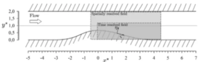
Fig. 2. Test section containing the two-dimensional bump geometry and the Piv fields of interest. The symbol⋆denotes the half height normalization. η represents the direction of the local outward normal of the surface andςthe tangential direction.

2.2. Measurement techniques

The unsteady separation process and its associated instability mechanism are known to be sensitive to small perturbations. Therefore, in order to preserve the flow physics, all the ex-perimental techniques employed in the present study are non-intrusive.

Velocity time-series measurements are carried out with a laser Doppler anemometry (Lda) system, mounted on a traverse device. The system consist of the fiberoptic-based optics and its electron-ics (Dantec Flowlite). Due to a solid wall close to the channel, a back-scatter orientation is used. Signal processing is performed via a Dantec Bsa Flow software. For all optical techniques, the

liquid is seeded with micron-size Iriodin1 particles with mean

particle diameters on the order of 10–15

µ

m, with a Stokes

number Stk (defined as the ratio of the characteristic time of

the particles,

τ

p to a characteristic time of the turbulent flow,

τ

f) approximatively in the range from 0.001 to 0.01.

Further-more, the relaxation time of the particles it is defined as:

τ

p

=

(

ρ

p

−

ρ

f)d2p

/

(18

µ

f) where

µ

f is the water dynamic viscosity,

ρ

p,

ρ

f respectively the particle and the water densities and dp the

mean particle diameter. Concerning the characteristic time of the

flow, defined as:

τ

f

=

η

f

/

Uc where

η

f is an estimation of the

Kolmogorov scale and Ucthe convection velocity estimated to be

equal respectively to 0

.

001H and 10% of the free-stream velocity.

As a consequence, the flow tracer fidelity in our particle image velocimetry experiments are acceptable since response time of the particles to the motion of the fluid is reasonably short to accurately follow the flow. The velocity profiles are measured at several locations along the test section during 5 min at each point of the profile. Spectral analysis of velocity signals is performed to uncover organized flow structures and determine their charac-teristics. In this particular case, the associate velocity time-series measurements are carried out with a longer time of 1 h each.

For quantitative flow visualization measurements, both a time-resolved and spatial-time-resolved Piv systems are used. Two different Piv setups are used in the present study. Both fields of view

are illustrated inFig. 2, the

⋆

symbol will denote hereafter the

half height normalization. The cameras are located on the side of the bump. The same particles are used for the Piv and the Lda measurements. The time-resolved setup is used to resolve the dynamic of unsteady vortices induced in the separation area, while the other setup increases the field of view in order to capture the near-wall phenomena with a good spatial resolution. The time-resolved system consists of a Quantronix Darwin-Duo operating at 528 nm with two-cavities laser and a 12 bit Imager Phantom v641 Cmos camera. The camera is able to operate in a single-frame mode with a frame rate of 1450 Hz at full resolution

(2560

×

1600 pixels). The laser beam is collimated and then

expanded into an approximately 0.5 mm in thickness sheet. 1 _{Pigments sold by Merck Corporation.}

The images are recorded at 1450 frames per second in order to have a sufficient temporal resolution to resolve the unsteady vor-tices dynamic. This set consists of 3000 instantaneous realizations

over a period of 2.07 s. The field of view is 12

×

45 mm2_covering

the entire channel height. The velocity vectors are calculated

using an adaptive correlation with 32

×

32 pixels interrogation

windows and a 50% overlap leading to a spatial resolution of 0.02H. A local median method, included in the Piv software, is

employed to eliminate outliers. A 3

×

3 median filter is also

used to smooth the vector fields in order to define the vortical structures in the separated area. An other Piv system was used to obtain a more spatially resolved velocity fields using a larger Ccd camera. In this setup, the light sheet is provided by a double-pulsed Nd-Yag laser Quantel Bslt220 with a 12 bit Imager

Pow-erview 16m camera at the full resolution of 4864

×

3232 pixels.

In those measurements, the data consist of ensembles of 1500

realizations recorded at 1 Hz. The field of view is 20

×

50 mm2

covering the full separation area. At the final stage, the

interro-gation window size was set to 16

×

16 pixels, corresponding to a

spatial resolution of 0.08 mm (0.008 H). The relative uncertainties on the mean velocity and on the fluctuation velocity can be estimated respectively to 0.2% and 2% of the free stream velocity. This study also focuses on the ability of the

electrochem-ical method (see [37] for a thorough review) to analyze the

wall-shear stress fluctuation distribution on the bump surface. The experimental method determines the limiting diffusion cur-rent at the surface of a platinum microelectrode and it was adapted to study the wall bounded turbulent flow dynamics

[35]. The wall-shear stress is experimentally determined using an

array of two-segment electrodiffusion microelectrodes (100

µ

m

×

500

µ

m) placed at different positions above the bump surface

(reported inTable 1). The segments are oriented with the longer

side perpendicular to the mean flow direction. The two probe

seg-ments (introduced by Son and Hanratty [38]) are able to measure

the magnitude of wall shear rate, detect the existence of near-wall flow reversal [39,40] and estimate the wall-shear rate signals

close the reattachment point [41]. The electrolytic solution used

in the present study is a mixture of ferri-ferrocyanide of

potas-sium (10 mol/m3) and potassium sulphate (240 mol/m3). The

limiting diffusion current is converted to voltage using a Keith-ley 6514 system electrometer, and acquired using a 12 bit A/d converter from an acquisition system Graphtec Gl1000. Wall-shear stress time-series measurements are sampled at 1 kHz using a 500 Hz low-pass anti-aliasing filter during 1 h each. For high-frequency fluctuations of the wall shear rate, the filtering effect of the concentration boundary layer reduces the mass transfer rate fluctuations enabling the use of the linearization the-ory [42–44]. For an accurate evaluation of the relative wall-shear stress fluctuation, the dynamic behavior can be corrected using the inverse method. This technique is a diffusion–convection

equation developed by Mao and Hanratty [45], its methodology

for heat transfer problems can be found in literature [46–49]. In our case, the inverse method, based on a sequential estimation ensures a sufficiently good frequency response (above 500 Hz) to resolve dominant frequency peaks and wall-shear stress statistics.

2.3. Flow conditions

In order to define the inflow conditions, experimental velocity measurements were recorded; using Lda, at an unperturbed

up-stream position of x⋆

= −

6 (we recall that x⋆is associated with

quantities non-dimensionalized by H and the origin is taken at the crest of the bump). Profiles of the streamwise velocity as a

function of the wall-normal coordinate are presented in Fig. 3

for a range of Reynolds number from 125 to 730. The profiles

obtained, specially at a Reynolds number of Re_τ

=

605, agree well

with the Dns results from [36], denoted inFig. 3with dashed line. The parameters of the upstream velocity profiles are presented in

Table 2.

Table 1

Flush-mounted micro-electrodes locations against the Reynolds number based on the friction velocity. LRdenotes the separate length and x⋆denotes the probes

positions normalized by the half height.

x⋆ 0.22 0.52 0.62 0.72 0.92 1.03 1.12 1.32 1.42 1.52 Reτ x/LR 125 0.07 0.17 0.21 0.24 0.31 0.34 0.38 0.44 0.48 0.51 165 0.10 0.23 0.27 0.31 0.40 0.44 0.49 0.57 0.62 0.66 255 0.13 0.30 0.35 0.41 0.53 0.58 0.64 0.75 0.81 0.87 375 0.18 0.43 0.52 0.60 0.77 0.85 0.93 1.10 1.18 1.27

Fig. 3. Profiles of the streamwise velocity against the wall-normal coordinate for various Reynolds-numbers. Dashed line represents Dns results of [36] at

Reτ=617.

3. Numerical method and theoretical background

3.1. Numerical procedure

Direct numerical simulations (Dns) of converging–diverging channels have been performed, with the exact same geometry, for three Reynolds numbers using the code Mflops3d

devel-oped by Lml. The parameters of the Dns are given in Table 3.

The algorithm used for solving the incompressible Navier–Stokes equations is similar to the one described in Marquillie et al.

[7]. To take into account the complex geometry of the physical

domain, the partial differential operators are transformed using mapping, which has the property of following a profile at the lower wall with a flat surface at the upper wall. Applying this mapping to the momentum and divergence equations, the mod-ified system in the computational coordinates has to be solved in the transformed Cartesian geometry. The three-dimensional Navier–Stokes equations are discretized using respectively eight and fourth orders centered finite differences for the first and second order derivatives in the streamwise x-direction. A pseudo-spectral Chebyshev-collocation method is used in the wall normal

y-direction. The spanwise z-direction is assumed periodic and is

discretized using a spectral Fourier expansion. The resulting 2d-Poisson equations are solved in parallel using Mpi library. Implicit second-order backward Euler differencing is used for time inte-gration, the Cartesian part of the diffusion term is taken implicitly whereas the nonlinear and metric terms (due to the mapping) are evaluated using an explicit second-order Adams–Bashforth scheme. In order to ensure a divergence-free velocity field, a fractional-step method has been adapted to the present formula-tion of the Navier–Stokes system with coordinate transformaformula-tion. In order to ensure a divergence-free velocity field a fractional-step method has been adapted to the present formulation of the Navier–Stokes system with coordinate transformation. The

Table 2

Mean-flow parameters. The subscript c and b referred to quantities based on the centerline and on the bulk velocity.

Uc(m s−1) Ub(m s−1) uτ (m s−1_{) Re} b(Ub×H/ν) Reτ Cfb×103 Symbols 0.26 0.21 0.0144 3 652 125 9.40

•

0.36 0.29 0.0190 5 010 165 8.70

◦

0.56 0.48 0.0295 8 330 255 7.59 0.72 0.62 0.0370 10 765 320 7.09 0.88 0.76 0.0430 13 265 375 6.38 1.02 0.89 0.0505 15 600 440 6.34 1.16 1.01 0.0565 17 565 500 6.26 1.32 1.15 0.0640 20 090 555 6.14 1.45 1.30 0.0695 22 575 605 5.74 1.61 1.43 0.0760 24 870 660 5.65 1.79 1.59 0.0837 27 650 730 5.54 Table 3

Dns parameters: uτ is the friction velocity, Ub is the bulk velocity, Lx & Ly & Lz are domain size in streamwise, vertical and spanwise directions, Nx & Ny& Nz are the number of grid points in the corresponding directions and x∗is the

streamwise coordinate of the inlet.

Reτ uτ Ub Lx Ly Lz Nx Ny Nz x∗ 187 0.0576 0.913 4π 2 2π 768 129 384 −5.21 395 0.0501 0.907 4π 2 π 1536 257 384 −3.67 617 0.0494 0.905 4π 2 π 2304 385 576 −5.21 Table 4 Separation points x∗ s, reattachment points x ∗

r and separation lengths L

∗

R for

experimental and Dns results.

Experimental data Dns data

Reτ L∗ R x ∗ s x ∗ r Reτ L ∗ R x ∗ s x ∗ r 165 2.388 0.564 2.952 187 2.917 0.538 3.455 375 1.198 0.510 1.708 395 1.187 0.565 1.752 605 0.764 0.500 1.364 617 0.838 0.547 1.385

metric of the Poisson equation for the pressure correction is taken explicitly and, in practice, few iterations are necessary to recover a pressure correction up to the second order in time which is the overall accuracy of the time marching algorithm. A constant

advection condition Uc based on the bulk velocity is used for

the outlet and inlet are generated from precursor Dns or highly resolved Les of flat channel flows at Reynolds number equivalent to each Dns of converging–diverging channels. The two boundary conditions only affect the property of the flow in very limited region far from the region of interest.

The inlets are generated from flat channel flows Dns at Reynolds number equivalent to each Dns of converging–diverging channels except for the medium Reynolds number case for which the precursor simulation was a highly resolved Les which does not affect the turbulence statistics in the region of interest subjected to pressure gradient Marquillie et al. [7] and Laval et al. [36].

4. Baseline mean flow description and statistical behavior

It is known, from various experiments [23,24,32], that the

separation bubble intermittently changes shape and size with the flapping of the shear layer and strongly depends on the flow regime. In order to establish the characteristics of the separated flow in the channel, we analyze the statistical behavior associated with the velocity fields and the wall shear-stress along the bump at the middle plane of the channel. In this section, numerical and experimental description of flow patterns, such as the separation length or the vorticity thickness, are extracted and compared to the numerical predictions.

4.1. Velocity fields and separation length

The recirculation zone, also referred as the separation bubble, is primarily dominated by a large two-dimensional vortex with a low circulation velocity. In order to visualize the baseline separate

flow fields,Fig. 4shows the normalized mean streamwise velocity

U

/

Ubfor both experiments and direct numerical simulations. To

have a validation of the numerical data, a comparison between experimental measurements (mean velocity contours from Piv at

Re_τ

=

165, 375 and 605) and numerical simulations (Dns for

Reynolds number Re_τ

=

187, 395 and 617) was done. The domain

that is considered

−

0

.

3

<

x⋆

<

4

.

5 and 0

<

y⋆

<

2 is the same for both the experiments and simulations. Values of the

separation lengths LR, separation point xsand reattachment point

xr for both the numerical and experimental data can be found

inTable 4. High levels of mean streamwise velocity distributions

are nearby the bump crest. Furthermore, for Re_τ

=

165

/

187, the

shear layer extends from the bump crest (x⋆

=

0) to x⋆

≈

4.

This value significantly decreases for Re_τ

=

375

/

395 and Re_τ

=

605

/

617, extending downstream the bump crest up to x⋆

≈

2

and x⋆

≈

1

.

5, respectively. The shear layers associated with the

latter are significantly thicker than those at Re_τ

=

165

/

187.

The location and length of the shear layers for both simulation

and experiment are similar, except for Re_τ

=

165

/

187 where

a slight difference occurs probably due to spanwise confinement

effects [50]. These similarities reveal a good agreement for mean

flow properties associated with the recirculation region between

experiments and Dns. The separation length (LR) is plotted in

Fig. 5for all the Reynolds-numbers studied in the present paper, including those from previous numerical investigations (Schiavo et al. [51]).

As already mentioned, it is crucial to predict if a separation exists considering the Reynolds number and the nature of the flow. For that, two cases are observed: no separation (not rep-resented herein) and a separation with reattachment over the bump surface. The recirculation zone behind the bump can be extracted from velocity measurements. The separation length

decreases up to an estimated critical value close to Re_τ

=

1200.

Marquillie et al. [7] observed that, for Re_τ

=

395 and Re_τ

=

617, the turbulent flow slightly separates on the profile at the lower curved wall and is at the onset of separation at the opposite flat wall (but keeping a positive minimum friction velocity of the order of 0.001 and 0.0015 respectively). The slowing down of the opposite wall is also noticed for the present experiment for all

the Reynolds numbers studied (seeFig. 4). This confirms a close

agreement between the numerical and experimental results and an accurate prediction of the separation bubble. The presence of a negative level of the mean tangential component of the

velocity distribution (U_ς), in the vicinity of the bump surface,

highlights the presence of a separation bubble caused by adverse pressure gradients. The development of the normalized mean

Fig. 4. Contour plots of normalized streamwise velocity (U/Ub): (a) Piv at Reτ=165; (b) Dns at Reτ=187; (c) Piv at Reτ =375; (d) Dns at Reτ =395; (e) Piv at

Reτ =605; (f) Dns at Reτ=617. Black arrows denote the separation points and white arrows the reattachment points. Dashed lines denote the separation bubbles for all the cases presented.

Fig. 5. Normalized separation length, L⋆_R, plotted against Reτ. Cross diamond symbols represent the present Dns data and cross square symbols represent the Les data from [51]. The uncertainty interval of LRbased on the Piv uncertainty

is equal to L⋆_R= ±0.1.

tangential component at the channel centerline (z⋆

=

0) for

Re_τ

=

165

/

187 can be seen in Fig. 6. The profiles are scaled

by the bulk velocity. The direction of the local outward normal

of the surface (

η

) is normalized by the separation length. Two

main features can be observed in the mean velocity profiles: the development of the recirculation area over the bump surface and the shear-layer generated by the bump crest on the profiles near

the wall (seeFig. 4). Once more, similar patterns are observed

for both experiment and simulation. The negative level close to the wall depicts a large recirculation area for Re_τ

=

165

/

187. This

area decreases for higher Reynolds-numbers (seeFig. 4).Fig. 4(a)

and (b) show a similar normalized flow profiles in the separation area, even though the separation length is not exactly at the same position along the bump.

The free shear layer plays an important role in the dynam-ics of the separated bubble, since the interaction of large eddy

structures with the wall in the reattachment region are formed upstream this area. Therefore, it is worth analyzing the stream-wise evolution of the shear layer characteristics. The growth of the separated shear layer may be described by the vorticity

thickness,

δ

_ω, as defined by Brown and Roshko [17] and given by:

δ

ω(x)

=

max_η

(

∆U_ς

∂

U_ς

/∂η

),

(1)

where ∆U_ς is the difference between the maximum

wall-tangential velocity on the high speed side of the shear layer,

U_ςmax, and the minimum wall-tangential velocity on the low

speed side, U_ςmin.

η

denotes the direction of the local outward

normal of the wall. Upstream the reattachment point ((x

−

xs)

/

LR

<

1), Uςmin reaches negative values in the reverse-flow

region and U_ςmax increases over the bulk velocity, Ub, up to 50%

(seeFig. 6). Two regions are evidenced in the streamwise evolu-tion of the vorticity thickness, seen inFig. 6, for the experimental

data (Re_τ

=

165) and numerical simulations (Re_τ

=

187, 375

and 617). Note that the experimental extraction of the vorticity

thickness, for Reynolds numbers higher than Re_τ

=

165, is not

possible with a satisfying accuracy due to the narrow thickness of the shear layer. The first region is located between (x

−

xs)

/

LR

=

0

and 0.4 where the growth of the mixing layer is exponential as predicted by linear stability theory in the case of planar mixing layers. The second one ((x

−

xs)

/

LR

>

0

.

4), evidenced inFig. 6and

obtained from our experimental data, is wider and characterized by a nearly linear rate d

δ

_ω

/

dx

=

0

.

17

−

0

.

275. The value obtained with the lowest Reynolds number is higher than those observed in classical planar mixing layer where the growth rate was equal to 0.17 ([52]). For (x

−

xs)

/

LR

≈

1, the shear layer is affected

by the reattachment process and the vorticity thickness reaches a maximum value before it strongly decreases. This result is in accordance with the observations of Cherry et al. [14] (seeFig. 8). In order to validate the Dns results, a comparison, shown in

Fig. 6. Normalized mean tangential component Uς at the channel symmetry plane (z⋆=0) againstη/LR. The direction of the local outward normal of the surface

for Reτ =165/187. The inset plot is the normalized vorticity thickness against (x−xs)/LR, xsdenotes the separation abscissa.#represent experimental data for Reτ=165. Lines represent numerical data (solid line; Reτ =617, short-dashed lines; Reτ=395 and medium-dashed lines; Reτ=187).

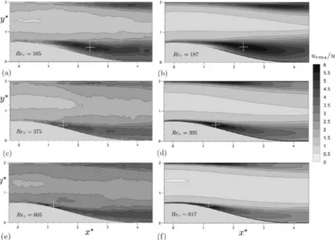
Fig. 7. Contour plots of normalized streamwise r.m.s. velocity (urms/uτ): (a) Piv at Reτ=165; (b) Dns at Reτ =187; (c) Piv at Reτ=375; (d) Dns at Reτ=395; (e)

Piv at Reτ=605; (f) Dns at Reτ=617.

focus on the normalized streamwise r.m.s. velocity fluctuations

for three equivalent Reynolds numbers i.e. Re_τ

=

165

/

187,

375

/

395 and 605

/

617. A global agreement can be observed

be-tween the experiments and the numerical results. The location of the highest r.m.s values for the three Reynolds number is denotes inFig. 7by a white cross symbol. For Re_τ

=

165

/

187, the peak locations and magnitudes for the simulation and the experiment

agree well. However, at Re_τ

=

375

/

395 and Re_τ

=

605

/

617, the

peaks are correctly located, but the magnitudes at the vicinity of the bump surface are lower for the experiments than for the simulations. This is due to the limited resolution of Piv with respect to the smallest coherent structures. A detailed analysis of the vortices in 2d planes of the Dns at the largest Reynolds

number (Re_τ

=

617) has been performed. Both experiments and

Dns exhibit the same general behavior for fluctuations. At Reτ

=

605

/

617, the separation area is significantly shorter and thicker

than at Re_τ

=

165

/

187 while the overall form of the distribution

Fig. 8. Distribution of the ratio∆PIV_{/ηfor Re}

τ=605/617.

at Re_τ

=

165

/

187 is similar to that at the higher

Reynolds-number. The loci of the r.m.s. maxima has moved upstream from

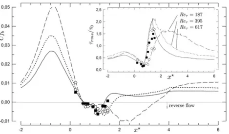
Fig. 9. Skin friction coefficient over the bump surface plotted against x⋆for three Reynolds-numbers (numerical and experimental dataset). Relative intensity of the wall shear-stress fluctuations are also plotted against x⋆.τ0denotes the mean wall shear stress evaluate at x⋆= −6.

◦

Reτ=165, Reτ=375 and Reτ=605. Lines represent numerical data (solid line; Reτ=617, short-dashed lines; Reτ=395 and medium-dashed lines; Reτ =187).

4.2. Behavior of the wall-shear stress statistics

The mean skin friction coefficient over the bump surface is

plotted against x⋆ in Fig. 9for Re_τ

=

165, 375 and 605. This

figure includes also Dns results at Reτ

=

187, 395 and 617

for comparison purposes. Statistical values are deduced from the wall-shear stress time histories using the electrochemical

technique at the streamwise locations defined in Table 1. The

mean skin friction obtained from experimental data agrees with the simulation. Measurements confirm the high value of the skin friction coefficient before the crest region. The separation region is also underlined by secondary peaks values observed from the

Dns data just after the bump crest at x⋆

=

2

.

3, 1.4 and 1.2,

for Re_τ

=

165

/

187, 375

/

395 and 605

/

617 respectively. These

peaks correspond to the maximum values of the streamwise

r.m.s. velocity denoted by cross symbols inFig. 7. Moreover, the

present results show a strong Reynolds number dependence and a trend toward a constant value, indicating that the flow reaches equilibrium conditions.

In order to quantify the near wall unsteadiness, the r.m.s. wall-shear stress above the bump is analyzed. The relative intensity of the wall-shear stress fluctuations over the bump surface, given in the inset ofFig. 9, is reported against x⋆for experimental and numerical data. Despite a slight shift of the friction coefficient in the separation region, the latter figure shows that the exper-imental results agree well with the numerical simulations. This minor difference is due to the limiting experimental frequency responses of the electrochemical technique, that are not able to reproduce correctly the high unsteadiness levels occurring at the reverse flow region. Low fluctuations of the wall-shear stress are observed before the separation. These fluctuations increase at the

separation region and remains high until x⋆

≃

6 for the lower

Reynolds numbers. Strong secondary peaks of the mean bulk skin friction coefficient, previously mentioned, coincide with the minimal values of the relative intensity of the wall-shear stress fluctuations.

5. Study of the dynamics of separated turbulent flow

5.1. Shedding and non-linear interactions of shear layer eddies

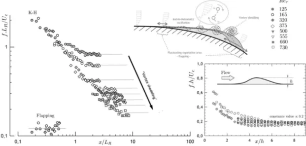
In order to enhance the dominant scales, for each region of the flow, and to investigate the characteristic frequencies embedded in the unsteady separated flow fields, we perform spectral anal-ysis at various locations along the bump for different Reynolds

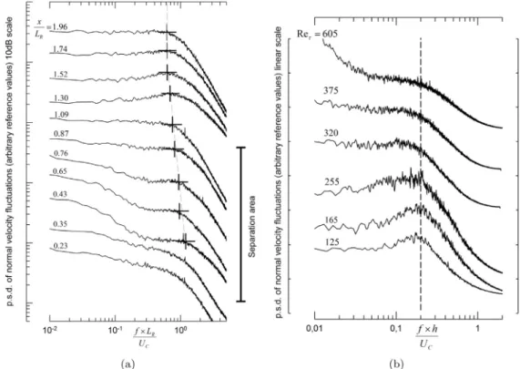
numbers. Power spectra densities (P.s.d) of the vertical fluctu-ating velocity component are sensitive to instability phenomena associated with spanwise structures. Therefore, we use P.s.d of the vertical velocity component in order to investigate the de-velopment of shear layer instabilities. P.s.d are computed using the Welch method with a Hamming window, an overlap of 75% and an acquisition time of 1 h each. Normalized P.s.d for various representative locations are presented in a logarithmic scale in

Fig. 10a for the streamwise stations inside the separation area.

For Re_τ

=

165, the frequency distribution exhibits a broadband

hump phenomenon, denotes by a

+

symbol in figureFig. 10a. In

particular, the humps are shifted toward lower frequencies when probes locations are moved from x

/

LR

=

0

.

43 to x

/

LR

=

1

.

52. For

1

.

5

<

x

<

1

.

8, the humps are centered around a fixed frequency. When rescaled by the bump height and for Reynolds numbers

ranging from 125 to 255, the fundamental frequency is St

≈

0

.

2

(where the centerline velocity Ucis considered) of the same order

than the vortex shedding phenomenon reported in the literature for various flow configurations (Sigurdson [18]). For Re_τ

>

320,

Fig. 10b shows that the humps are broader and less defined than those obtained for lower Reynolds numbers. These observations indicate that the shape and motion of vortices becomes more irregular for higher Reynolds numbers (i.e. the vortex-shedding acts in broadband frequency).

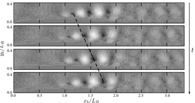
A sequence of characteristic snapshots of the spanwise

com-ponent of the fluctuating vorticity

ω

z from time-resolved Piv

measurements is shownFig. 11for Re_τ

=

125. The local

fluc-tuating vorticity is used herein to identify vortices in the flow field and to show that the main dominant large structures are de-formed, sheared, broken, and periodically transported along the shear layer. This figure illustrates the development and the spatial organization of the vortex-shedding from the shear layer. The negative fluctuating spanwise vorticity corresponds to clockwise rotation of the vortices, as the positive fluctuations correspond to the counter-clockwise rotation. For this Reynolds number,

Re_τ

=

125, the propagating vortices are nearly circular with a

radius of approximately H

/

2 stretching into elliptical shapes

fur-ther downstream. This phenomenon is also previously observed by Mollicone et al. [10].

The fluctuating spanwise vorticity field, shown inFig. 11(a–

e), consists of alternate regions of positive and negative values. A vortex structure convection without self-interaction but with

a strong collective interaction [52] can be observed. A region of

high vorticity inside the shear layer shows that the structures re-main dissociated during a cycle. White circles represent the cores

Fig. 10. Power spectral densities (P.s.d) of the vertical fluctuating velocity component,v′_{, (a) at various x/L}

Rlocation along to the shear layer and at an elevation

corresponding to the maximum of the velocity gradient locations for Reτ=165 (b) at x/LR≈1.5 for various Reynolds numbers. h/UCis used in order to normalize

the frequency and P.s.d are plotted with arbitrary reference scale. Measurements are obtained from the laser Doppler anemometry. The+symbol denotes the evolution of spectral emergences against the dimensionless probe positions. Measurements are obtained from the laser Doppler anemometry.

Fig. 11. Two samples of the fluctuating vorticity field from the Tr-Piv at Reτ =125 showing different phases of the same shear layer vortex without (a to e) and with (f to j) self-interacting. Time steps follow from top to bottom and the normalized time interval between snapshot is∆t.Ub/h=0.0216. Arbitrary scale.#

denotes dominant vorticity centers. The two vortices cores pointed out have a clockwise rotation.

of the propagating vortices for different consecutive time instants. The vortex core is defined as the position of the maximum mag-nitude of the spanwise vorticity. These cores are initially located closer to the centerline of the shear layer. The lines connecting the vortex cores correspond to a typical path followed by the shed

vortices. The relatively uniform spacing between vortex cores is attributed to an almost constant vortex shedding frequency, which also confirms that the vortex-shedding moves with a con-stant convection velocity. The general features of unsteady events

the period, the vortex size and shape and the self-interaction, vary substantially from one structure to the next. An example of coher-ent structures interaction is illustrated inFig. 11(f–j). Based on the mechanism observed previously, it is expected that the identified vortices (with clockwise rotation) convect without further inter-action. But, in this case, the vortex-shedding, which is driven by the low frequency oscillation, subsequently diverges away. This behavior is due to the reverse flow moving toward the wall lead-ing, in this particular case, to a merging of the coherent structures with the vortex development just downstream the shear layer. This phenomenon occurs more often when the Reynolds number increases and can explain the broadband behavior of the shedding for higher Reynolds numbers.

5.2. Low-frequency flapping

The influence of the mean recirculation region onto the low-frequency dynamics was identified in a very recent study carried

out by [53], for the shock/wave turbulent boundary layer

inter-action. In particular, the authors investigated the linear global stability of the mean flow obtained by LES. They found low frequency modes that are strongly localized in the recirculation area and exhibit close correspondence with the breathing of the bubble observed in the LES. In this context, the influence of the recirculation zone onto the low frequency motions is of major interest in the study of turbulent separated flows. Here-after, we investigate low-frequency dynamics (flapping motion) in the light of weighted power spectrum density of the wall-shear stress and characteristic scales of the mean separated flow. In

Fig. 12, weighted power spectral density distribution are shown

for several distances x

/

LRand Reynolds-number (Reτ

=

125, 165,

255 and 375). The hump, obtained by the power spectra of the normal fluctuating velocities in the shear-layer, correspond to the frequency of shear-layer vortices. However, other humps can be found at values lower than those obtained from the shear-layer vortices frequency. These humps, underlined by plus symbols in

Fig. 12, are clearly observed until x

/

LR

≈

0

.

6. For higher distances,

x

/

LR

>

1, the peaks seem to merge and disappear. As mentioned

previously, when the distance from the bump crest increase, the frequency range, associated to the shear-layer vortices, moves toward lower values. This deviation can be seen by the

dashed-lines in Fig. 12. In contrast to the high-frequency shear-layer

vortices, the low frequency humps are centered at a constant frequency St

=

0

.

12 (denoted by vertical dashed-lines inFig. 12).

This characteristic frequency is consistent with those obtained in

previous experimental studies ([14] and [12]) and corresponds to

the flapping of the shear-layer. The low flapping frequencies and shear-layer vortices appear to be confined near the bump crest region.

In figure12, we observe that the humps associated with both

flapping motion and vortex shedding phenomenon emerge for

probes localized in the recirculation region for 125

<

Re_τ

<

375. The humps flatten as the probes are moved away from the region associated with mean separation. This characteristic curve is in agreement with the measurements observed in a

sepa-rated bubble for a backward-facing step configuration [54]. These

broadband humps are less visible compared to a laminar flow regime, where it is easier to detect the phenomena (see Passaggia et al. [27]).

The broadband humps, which is characteristic of the flow spectra in the shear layers, vanishes downstream the shear layer. In the light of the present findings, the presence of flapping in this flow regime has not been detected before. Indeed, in the present study, the flapping could not be detected in the velocity spectra but it is revealed only in the wall shear stress spectra.

To give some insight about the driving mechanism and its link with mean flow properties, we use the model derived by

Pipon-niau et al. [21]. The latter model suggests an universal parameter

St

/

g(r)

≈ [

5

−

6

]

with: g(r)

=

δ

′ w 2 2(1

−

r) 1

+

r

(

(1

−

r)C

+

r 2

)

where

δ

′

w is the spreading rate of the mixing layer and r is the

reverse flow intensity. These values are associated with the

two-dimensional mean flow. In particular, Piponniau et al. [21] argue

that g(r) is a universal function relying on classical similarity properties of plane mixing layer. As underlined by Piponniau et al. [21], C is fixed to 0.14. In the latter expression, we neglect compressibility effects. When using mean quantities associated

with DNS database for Re_τ

=

165

,

395 and 617 we obtain for

St

/

g(r) values that are comprised between 4.75 and 5.4 for St

=

0

.

12. Hence, it may suggest that the two-dimensional mechanism

proposed by Piponniau et al. [21] that relies on an instantaneous

imbalance between the entrainment rate from the bubble and the reinjection of fluid near the reattachment line is also the driving process of the flapping phenomenon for a separated flow behind a bump.

5.3. Modal decomposition: Dmd analysis

In the previous section, the analysis of experimental data, to calculate the weighted power spectrum density of the wall-shear stress fluctuations, has shown two main points. First, the spec-trum is broadband, reflecting highly turbulent activity. Second, the two frequency ranges are statistically favored: the first one

at low frequency, St

∼

0

.

1, corresponding to a flapping dynamics

and the second one, St

∼

2, mainly linked to the dynamics

of the shear-layer generated by the separated boundary-layer downstream of the bump. The study of the dynamics of these two particular frequency ranges and in particularly the link be-tween the frequency and the spatial location of the associated mode can allow us to better understand the different physical mechanisms involved. Several modal decompositions can be used for this investigation, the most well known being the Proper Orthogonal Decomposition (Pod). The Pod allows to order modes by level of decreasing energy. However this is not our objective here because a frequency decomposition is more natural when we want to compare with experiments. Recently Rowley et al.

[55] and Schmid [56] proposed a Dynamics Modal Decomposition

(Dmd) which has the advantage to be a frequency modal

decom-position easily accessible (see Appendixfor a deeply study of this

technique). The advantage of the Dmd, relative to other frequency decomposition such as for example Fourier decomposition, is to better grasp the real physical mechanisms, in particular for tran-sient or non-equilibrium phenomena. The Dmd can be used with both experimental and numerical data. The main constraint is to have access to sufficiently time-resolved data. In the present case, experimental data is well resolved temporally over a long time, but poorly resolved in space, when the Dns data is well resolved both in space and time but limited to a short integration time. The objective is to characterize the spatial nature of the disturbance for a given frequency, this is why the Dmd analysis is performed on Dns data. This implies that only the medium frequencies are available, flapping phenomenon is then unresolved. The Dmd analysis was conducted only for the case with a Reynolds number

Re_τ

=

617.

The computational domain for Dmd analysis is linked to the bump in local coordinates system (xb

/

LR

,

yb

/

LR

,

zb

/

LR) and shown

in Fig. 13by a red rectangular box. The lengths of the domain are: (Lxb

,

Lyb

,

Lzb)

/

LR

=

(3

.

31

,

0

.

5

, π/

2). The computational grid

Fig. 12. Weighted power spectrum density of the wall-shear stress fluctuations at various Reynolds-number against the distance x/LR.+and×symbols denotes the

spectrum peaks. The vertical dashed line shows the normalized low-frequency 0,12 and the inclined dashed lines denotes the evolution of the secondary spectrum peaks. Measurements are obtained from the electrochemical method.

Fig. 13. Computational domain for Dmd analysis. (x/LR;y/LR) are the global

coordinates.(xb/LR;yb/LR)are the local coordinates linked to the bump.

The Dmd modes are processed as follows: (i) the numerical data initially given in global coordinates system (x

/

LR

,

y

/

LR

,

z

/

LR) are

interpolated in Dmd grid (xb

/

LR

,

yb

/

LR

,

zb

/

LR). (ii) The velocity

component (u

, v, w

) are decomposed into u

=

u∥

+

u⊥where u∥

and u⊥ are the parallel and perpendicular velocity components

to the direction of the mean flow U respectively. These two components are given by:

u∥

=

(

u

·

U

)

∥

U

∥

2 U and u⊥

=

u

−

u∥

.

(iii) The Dmd analysis was performed in the referential

(

xb

,

yb

,

zb

)

then projected in the referential

(

x

,

y

,

z

)

. Details of the method

are summarized in Appendix. The Dmd analysis is based on a

sequence of Ns

=

930 snapshots of the velocity field sampled at

a constant sampling period∆ts

=

0

.

06. Preliminary tests have

shown that these parameters (∆ts

,

Ns) are able to converge fairly

well the frequency range

[

0

.

1

;

10

]

.

Fig. 14-(Left) depicts the eigenspectrum of the approximate

Koopman eigenvalues

λ

j. Almost all eigenvalues lie on the unit

circle, indicating that the dynamics is statistically stationary and

well converged.Fig. 14-(Right) shows the kinetic energy of each

mode with respect to the associated Strouhal number St (in a

logarithmic scale). The turbulent nature of the flow generates a continuous field of peaks ranging from high to low frequencies. This result is in good agreement with the Psd analysis previously discussed. In the previous sections, the analysis of temporal sig-nals from the Dns has shown that there is a range of frequencies

around St

∼

2 where the dynamic implies coherent structures

related to the shear-layer. As this frequency range is well resolved by the Dmd analysis, it is thus possible to extract the Dmd mode

Fig. 14. (Left): Spectrum of the Dynamic Mode Decomposition. (Right): The normalized kinetic energy norm versus the Strouhal number. Reτ=617.

Fig. 15. The Dmd mode for St=2 computed from the flow around the bump,

illustrated using two opposite contours of the perpendicular velocity component

u⊥.

for this particular frequency.Fig. 15depicts the spatial

distribu-tion of the Dmd mode for St

=

2 and for the wall normal velocity

component. The velocity field of the Dmd mode is clearly related to a Kelvin–Helmholtz mode with a parallel wavelength of about

Fig. 16. Evolution of the perpendicular component of velocity of the (K–H) mode for a Strouhal number St=2 over one period T .

of the bump, the K–H mode is almost two-dimensional in the first part of the separated zone. In this area, the mode is spatially amplified. Further downstream, the K–H mode quickly loses its two-dimensional nature and complex three-dimensional struc-tures are observed that quickly lose their coherence. As shown in the next section (Fig. 17), this zone is characterized by a vortex-shedding phenomenon where the frequency no longer evolves with the streamwise direction. The frequency of vortex-shedding is determined by the value of the frequency of the K–H mode when the vortex-shedding starts. This abscissa where the K–H modes are released depends on the frequency. The higher is the frequency, the earlier the vortex-shedding phenomenon starts. In order to clearly identify the nature of the modes in the first part of the separated zone, the computation of the convection velocity of

these modes has been achieved.Fig. 16shows the evolution of the

Kelvin–Helmholtz mode at St

=

2 over one period T . To improve

the coherence of the mode, the velocity field has been previously averaged in z direction. The advection velocity of the structures

is closed to Uc

/

2, which corresponds perfectly to the convection

velocity of shear-layer instabilities observed in the literature. One may also remark some similarities between the modes obtained by the Dmd analysis carried out in the present study for a turbulent flow and the global modes computed by Ehrenstein

and Gallaire [24] in a laminar regime for the same flow case.

It suggests the persistence of such instabilities in the turbulent regime.

6. Conclusion and final remarks

The present analysis combining numerical and experimen-tal approaches aimed to deeply understand how the Reynolds-number affects the mean separation length and how the turbulent regime may change flow unsteadiness characteristics. The re-sults indicated that, for turbulent flows, the frequency range is the typical combination of flapping phenomenon and shear-layer instabilities. High-resolution Piv and electrochemical mea-surements have been conducted in a Reynolds-number range of 125–730. These results were compared to direct numerical

simu-lations, at similar Reynolds numbers (Re_τ

=

187

,

395

,

617). Flow

baseline statistics from both simulations and experiments were compared in order to validate the Dns prediction. The velocity fields along the bump were analyzed and showed the existence of a separated region, clearly observed for moderate Reynolds numbers. A deep analysis of self-sustained oscillations and con-vective instabilities of the shear-layer was also addressed. Two high frequency shear layer instabilities, shedding phenomena and K–H oscillations, and one low-frequency, flapping motion, are identified. Both Psd of vertical velocity component and wall shear stress were used to investigate unsteadiness of the separate shear layer. It showed that characteristic frequencies detected for low

Reynolds numbers and classically observed in the literature, still exist for high Reynolds numbers. A peak at the fundamental frequency corroborated the existence of shedding of the shear layer vortices. Weighted power spectrum density of the wall-shear stress fluctuations were computed to investigate the near wall unsteadiness. Flapping frequencies could only be detected in the wall shear stress spectra, and appeared to be confined near the crest bump region. Results showed a broadband spectrum and two frequency ranges statistically being favored. This broad band peak can be explained by the non-periodic self-interacting vortex pairing phenomena; observed from the Tr-Piv measurements.

Considering the substantial variation of flow characteristics within the investigated range of Reynolds numbers, a length scale, linked to the separation length flapping phenomenon, as opposed to a geometric model dimension, would be more

ap-propriate. Frequency peaks, extracted from Figs. 10 & 12 for

all the Reynolds-numbers, as a function of x

/

LR are plotted in

Fig. 17. For this case, the flapping exhibits a nearly constant

normalized low-frequency of St

=

0

.

12. Variations of

Reynolds-number influence the instability. For values of St around 2, the

shear-layer vortex frequencies decrease due to the shear-layer instabilities and are strongly dependent of the Reynolds-number. Investigation on both experimental and numerical data did not yield to provide suitable scaling for the shear-layer instabilities, because the very restricted region where the phenomena occurs, for high Reynolds numbers, is difficult to analyze. However, in our case, the frequency of this phenomena can be scaled by the vorticity thickness. This scaling led to a same dimensionless frequency value f

δ

_ω

/

UC

≈

0

.

1

±

0

.

02 for the three lower Reynolds

numbers, but the latter is lower compared to those classically obtained in the literature. We propose the bump height, H, as an alternative length scale for the shedding scaling. The variation

of the resulting universal normalized frequency fh

/

Uc is shown

in the upset of Fig. 17 . This scaling dramatically reduces the

variation of the scaled vortex shedding frequency. A summary of the experimental results obtained in the present study is reported inFig. 17. In fact, despite a minor scatter, the data collapse into

a universal normalized frequency of about fh

/

Uc

≈

0

.

2, which is

in good agreement with that reported in the literature.

From these analyses, it appears that unsteadiness observed for the same configuration in the laminar regime by Passaggia et al. [27] are also detected in the turbulent regime. Nevertheless, some discrepancies exist. For instance, the flapping phenomenon

is of the order St

=

0

.

12 in the turbulent regime. When

con-sidering the laminar case studied by Passaggia et al. [27] we

obtained St

≈

0

.

5 which is significantly higher. It suggests that

a different mechanism as the one proposed by Gallaire et al.

[32] occurs in the turbulent regime. In addition, the good

agree-ment between dimensionless frequency derived from the model

given by Piponniau et al. [21] and results provided by the same

authors gave some confidence that a two-dimensional mecha-nism based on fluid entrainment along the mixing layer is also active for this configuration. The latter mechanism generates low-frequency motions associated with successive contractions and expansions of the recirculation zone.

It should be also consistent with the recent numerical study

carried out by Mollicone et al. [10] based on the DNS database

of Mollicone et al. [9] for a similar configuration. The previous

authors through the Generalized Kolmogorov equation GKE give further support onto a strong correlation between vortical struc-ture developing onto the shear layer and the recirculation region.

As underlined by Mollicone et al. [10], these coherent motions are

trapped by the recirculation region while being advected in the bubble. They may eventually disappear and reform again at the top of the recirculation area.

Dmd analysis was conducted for one numerical data set (Reτ

=