Mélange turbulent dans l'estuaire maritime du Saint-Laurent

MÉLANGE TURBULENT DANS L'ESTUAIRE MARITIME DU SAINT-LAURENT

Thèse présentée

dans le cadre du programme de doctorat en océanographie en vue de l'obtention du grade de Philosophiae Doctor

PAR

FRÉDÉRIC CYR @(!)@

Avertissement

La diffusion de ce mémoire ou de cette thèse se fait dans le respect des droits de son auteur, qui a signé le formulaire

«

Autorisation de reproduire et de diffuser un rapport, un mémoire ou une thèse». En signant ce formulaire, l'auteur concède à l'Université du Québec à Rimouski une licence non exclusive d'utilisation et de publication de la totalité ou d'une partie importante de son travail de recherche pour des fins pédagogiques et non commerciales. Plus précisément, l'auteur autorise l'Université du Québec à Rimouski à reproduire, diffuser, prêter, distribuer ou vendre des copies de son travail de recherche à des fins non commerciales sur quelque support que ce soit, y compris l'Internet. Cette licence et cette autorisation n'entraînent pas une renonciation de la part de l'auteur à ses droits moraux ni à ses droits de propriété intellectuelle. Sauf entente contraire, l'auteur conserve la liberté de diffuser et de commercialiser ou non ce travail dont il possède un exemplaire.

Cédric Chavanne, président du jury, Université du Québec

à

Rimouski

Daniel Bourgault, directeur de recherche, Université du Québec à Rimouski

Peter S. Galbraith, codirecteur de recherche, Institut Maurice-Lamontagne

Luc Rainville, examinateur externe, University of Washington

Science studies what's at the edge of understanding, and what 's al the edge of understan-ding is usually fairly simple. And it rarely reaches human affairs.

Noam Chomsky

Au moment où j'écris ces lignes, il est plus facile de poser un robot sur une comète que de faire une lutte efficace aux problèmes climatiques, environnementaux et sociaux. Vraiment, l'être humain est une drôle d'espèce ...

Petite histoire de doctorat...

Beaucoup de personnes sont passées (et restées) dans mon entourage au cours de mon doctorat. Quand je suis débarqué à l'ISMER le 3 mai 2009, James Caveen et Simon Sen-neville m'ont accueilli et installé dans le 0-240, le siège social du LASSO 1. Dans ce local bourré de meubles, deux étudiants étaient cachés: Pierre St-Laurent et Simon St-Onge. Ils ont su tout de suite m'intégrer. Ils étaient là aussi pour répondre à mes questions de débutant et si je les dérangeais, ça ne paraissait pas. Il y avait aussi Joanie, Virginie et Sylvain qui étaient sensés être là, mais ils n' y étaient pas souvent. Merci à eux aussi pour l'intégration.

Assez rapidement par la suite s'est enchaînée une suite de péripéties: feu à l'université, travaux de construction (qui durent encore aujourd'hui), déménagement dans un local en tapis plein de poussière, retour dans le 0-240, mais sans les fenêtres, changement de mobilier, etc.

À

travers tout ce chamboulement, le nombre d'étudiants a explosé. J'ai donc beaucoup de personnes à remercier pour l'ambiance du labo, trop pour tous les nommer, mais je suis sûr qu'ils se reconnaissent. Je tiens à remercier spécialement Paul, qui a traversé pas mal toutes ces étapes avec moi, ainsi que Camil et Thibault, deux autres qui ont aussi vu l'évolution du LASSO. Merci aussi à ceux qui étaient là quand je suis parti: Anne-Claire, Mélany, Benoit, Elliot, Julien, Robin.

Évidemment, un énorme merci à Daniel qui, à partir de Terre-Neuve, m'a invité à faire un doctorat avec lui. Nous sommes arrivés presque en même temps à Rimouski. Bien qu'il jouait son rôle de superviseur, j'ai eu l'impression d'avoir une relation d'ami et de

collabo-rateur avec lui, comme le démontre les nombreux projets parascolaires auxquels nous avons participé. Même chose pour Peter, partenaire principal de mes sorties de terrain au cours des-quelles les heures en mer ont permis un brassage d'idées intéressant. Les nombreux party

et soupers avec vous deux m'ont aussi montré un autre côté de la recherche plus détendu. Vous m'avez aussi montré à rester sur mes gardes avec vos questions-pièges, car vous vous rappelez longtemps des mauvaises réponses! Merci aussi au Fond québécois de recherche -Nature et technologies (FRQ-NT) qui a financé ma thèse et qui continue de me soutenir avec une bourse de post-doctorat.

Merci à Cédric Chavanne et Luc Rainville, respectivement président et examinateur externe sur le jury de thèse, ce fut un plaisir de partager de bons moments avec vous durant et après ma soutenance de thèse. Vos commentaires ont été très pertinents (et très flatteurs) et continuent de me faire réfléchir encore ajourd'hui. Ils sont aussi une motivations à continuer dans le domaine de la recherche. J'ai un merci spécial à faire à Dany Dumont et Frédéric Maps, deux jeunes chercheurs qui ont été, chacun à leur façon, une source d'inspiration pour mieux comprendre la recherche et à Joël Chassé pour avoir siégé sur mon comité de thèse. Merci aux techniciens qui m'ont aidé sur le terrain: Rémi, Bruno, Gilles et Sylvain.

En plus de ceux que j'ai cotoyés à l'université, il y a bien sûr les amis et la famille qui nous ont beaucoup aidés, Eveline et moi, dans notre tentative de concilier famille-rénovation-étude-plaisir. Notre passage à Rimouski fut tout aussi marquant au point de vue personnel. En plus des études, nous avons eu une maison centenaire à rénover et vécu l'arrivée d'une petite Flore. Merci à mes parents pour leurs nombreux coups de main et à Rose-Marie et Guillaume, nos colocs d'exception.

Finalement, merci Eveline de ne pas m'avoir largué en chemin. Je suis conscient que la vie avec moi n'est pas de tout repos, SUltout quand je suis en rush de travail. Je n'aurais peut -être jamais réussi si tu ne m'avais pas aidé de toutes les façons dont tu l'a fais. Flore, peut-être que tu ne liras jamais ces lignes, mais sâche que ta maman a été exceptionnelle pour permettre à papa de finir son doctorat. Merci

à toi

aussi d'être apparue si belle et si gentille dans notre vie de fou. Merci.

Entre 2009 et 2012, les premières mesures directes du taux de dissipation de l'énergie cinétique turbulente dans l'estuaire maritime du Saint-Laurent (EMSL) ont été effectuées avec un profileur vertical de micro-stmctures. Il s'avert que le mélange dans la couche li-mite de fond près des bords de l'EMSL est 10 fois supérieur à celui à l'intérieur, loin des bords et quatre fois plus élevé durant le flot par rapport au jusant. Il semble aussi que le mélange à la tête du chenal Laurentien, l'extrémité en amont de l'EMSL, soit quant à lui 300 fois supérieur au mélange intérieur. Avec l'aide d'observations historiques de température et de salinité provenant de la station de monitorage Rimouski, il a été démontré que l'érosion de la couche intermédiaire froide (CIF), c.-à-d. son mélange estival, est assuré à un tiers par des processus près des bords et aux deux tiers par des processus locaux, loin des bords. Les données d'un mouillage déployé le long des bords de l'EMSL suggèrent aussi que les déplacements verticaux de la CIF le long de la topographie en pente sont forcés par des marées internes générées à la tête du chenal Laurentien. L'utilisation d'observations histo-riques de concentration de nitrate dans l'EMSL combinées aux observations de turbulence a permis une estimation des flux verticaux turbulents de nitrates à la tête du chenal Laurentien ainsi qu'à la station Rimouski. Les flux à la tête du chenal sont 600 fois plus élevés qu'à la station Rimouski et peuvent à eux seuls soutenir la majeure partie de la production primaire hors bloom.

Mots clés : turbulence, mélange côtier, profileur vertical de micro-stmctures, es -tuaire maritime du Saint-Laurent, couche intermédiaire froide, marées internes, flux turbulent de nitrate.

Between 2009 and 2012, the first measurements of dissipation rates of turbulent kinetic energy in the Lower St. Lawrence Estuary (LSLE) were carried out with a vertical micro-structure profiler. Boundary mixing in the bottom boundary layer at a sloping boundary is 10 times higher compared to inner mixing far from boundaries and four times higher during the flood compared to the ebb. Mixing is also 300 times higher at the head of the Lauren-tian channel, a sill located at the upstream limit of the LSLE, compared to interior rnixing. Using historical temperature and salinity observations from the monitoring station Rimouski, it is shown that boundary mixing accounts for one-third of the erosion rates (i.e., warning by mixing) of cold intermediate layer (CIL). Interior mixing, i.e., mixing far from boundaries, accounts for the remaining two-thirds. Observations from a mooring deployed over the slo-ping boundary suggest also that the CIL undergoes swashjbackwash motions on the si ope in response to a forcing by internaI tides generated at the head of the Laurentian channel. The combination of turbulence measurements and historical nitrate concentration observations re-veals that turbulent nitrate fluxes are 600 times higher at the head of the Laurentian channel th an at the Rimouski station. Such fluxes can account for most of the post-bloom primary production in the LSLE.

Keywords : turbulence, coastal mlxmg, vertical microstructure profiler, Lower St. Lawrence Estuary, cold intermediate layer, internaI tides, turbulent nitrate fluxes.

RÉSUMÉ . . XI

ABSTRACT. Xlll

TABLE DES MATIÈRES. xv

LISTE DES TABLEAUX . XIX

LISTE DES FIGURES . . XXI

INTRODUCTION GÉNÉRALE ARTICLE 1

INTERIOR VERSUS BOUNDARY MIXING OF A COLD INTERMEDIATE LAYER Il 1.1 Abstract ..

1.2 Introduction

1.3 The Gulf of St. Lawrence 1.4 Datasets and methodology

1.4.1 CTD data . . . ..

1.4.2 Sea surface temperature (SST) 1.4.3 Turbulence measurements 1.5 Observations . .... .. . . ..

1.5.1 CIL characteristics and variability 1.5.2 Turbulence .

1.6 Heat diffusion model 1.6.1 Model description 1.6.2 Results 1.7 Discussion. 1.8 Conclusion 1.9 Acknowledgments Il 12 14 15 15 16 16 18 18 19 20 20 22 22 24 25

ARTICLE II

BEHAVIOR AND MIXING OF A COLD INTERMEDIATE LAYER NEAR A SLOP-ING BOUNDARY

2.1 Abstract.. 2.2 Introduction

2.2.1 The Lower St. Lawrence Estuary and internaI tides 2.3 Datasets and Methodology

2.3.1 Mooring data . . .

2.3.2 Fine- and micro-structure data 2.3.3 Phase averaging . . . .

2.3.4 Revisiting the Forrester internaI tide model 2.4 Observations . . . .

2.4.1 Cold intermediate layer behavior at the slope 2.4.2 A model for the propagation of internai tides 2.4.3 Mean turbulent quantities .. . . 2.4.4 High-frequency internai waves observations. 2.5 Discussion. . . . .. . .

2.5.1 CIL behavior in response to internai tides 2.5.2 Boundary mixing in the LSLE . . . . 2.5.3 Boundary mixing mechanisms and forcings 2.6 Conclusion .. . .

2.7 Acknowledgments ARTICLE III

TURBULENT NITRATE FLUXES IN A LARGE-SCALE ESTUARY . 3.1 Abstract ..

3.2 Introduction 3.3 Methodology

3.3.1 Nutrient concentration data . 3.3.2 Turbulence data .. .. . . . 41 41

42

42

44

44

45 47

48

50 50 53 55 57 59 59

60

61

66

67

81 81

82

85 85

86

3.4.1 Nutrient concentration

3.4.2 Turbulence observations and nitrate fluxes. 3.5 Discussion .. . . .. .. .

89

92

97

3.5.1 The nutrient pump mechanism 97

3.5.2 Contributions to the GSL nutrient budget 99

3.5.3 Nutrient pumping in sustaining primary production in the LSLE 101 3.6 Conclusion . . . .

3.7 Acknowledgments CONCLUSION GÉNÉRALE. RÉFÉRENCES . . . .. .. . ANNEXE A

CALCUL DU TAUX DE DISSIPATION DE L'ÉNERGIE CINÉTIQUE TURBULENTE 103 104 121 127 À PARTIR DU CISAILLEMENT . . . . . . . . . . . . . . . . . . . 143 ANNEXEB

EXPRESSION DU TAUX DE DISSIPATION DE L'ÉNERGIE CINÉTIQUE TURBU-LENTE EN CONDITIONS ISOTROPIQUES . . . .. . . 153

Slopes of linear best fits for Fig. 12. The three columns are respectively the CIL core temperature warming rate, the CIL thinning rate and the rate of in-crease in CIL heat content. Each is calculated for the climatology of CTD observations (1993-2010), the modeled temperature diffusion using respec-tively the interior diffusivity profile Ki and the mean diffusivity profile from

aU available casts Ka. 27

2 Mooring information 68

3 Turbulent nitrate fluxes in the World Ocean from previous studies (adapted from Bourgault et a1., 20 Il). The values reported are whether the flux through the nitracline, the base of the euphotic zone or the base of the mixed layer and are sorted from the lowest to the highest. . . . 105 4 Tableau récapitulatif des chiffres à retenir de la thèse (voir aussi la figure 42). 122

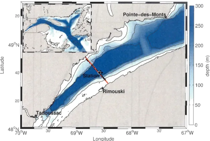
1 Carte bathymétrique du golfe (encadré) et de l'estuaire maritime du Saint-Laurent (EMSL). La tête du chenal Laurentien est identifiée par un encerclé. 2 Location of 892 VMP casts (black dots) and bathymetric features of the St. Lawrence Estuary (main figure) and the Gulf of St. Lawrence (inset). The black contour hnes are the 50, 150 and 250 m isobaths. Rimouski

sta-3

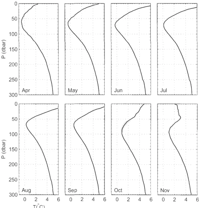
tion is identified with a white circle superimposed over the maximum profile concentration. The red line is the section referred to in Fig. l3 and where sampling was performed during 10 days in July 2010. . . . . . . . . . . . . . 27 3 Monthly mean temperature profiles calculated from April to November over

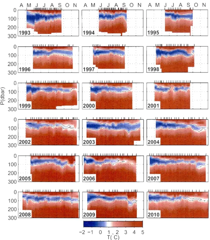
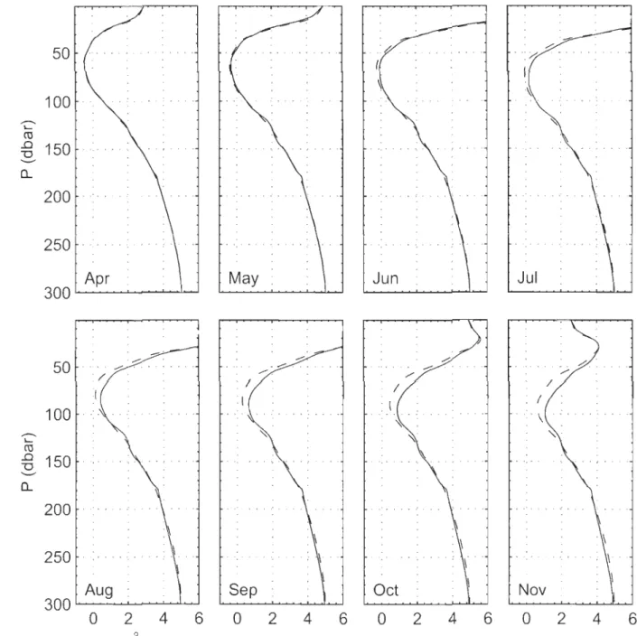
the period 1993-2010 from the CTD casts of Fig. 5. The gray shadings are the 95% confidence intervals . . . . . . 28 4 Monthly mean salinity profiles calculated as in Fig. 3. . 29 5 Evolution of temperature profiles from April to November, linearly

interpo-lated from 418 CTD casts that are indicated by lines at the top of each panel. To focus on the CIL, the color scale is saturated at SOC while summer surface temperature can reach more than 10°C, and 1°C isotherms are highlighted with a black contour. . . . . . . . . . . . . . . . . . . . . . . . . . . . . . . 30 6 April to November water temperature. a) Monthly climatology over the

pe-riod 1993-2010 calculated from the CTD casts of figure 5. b) Modeled evolu-tion of temperature using the observed mean interior diffusivity profile

K.

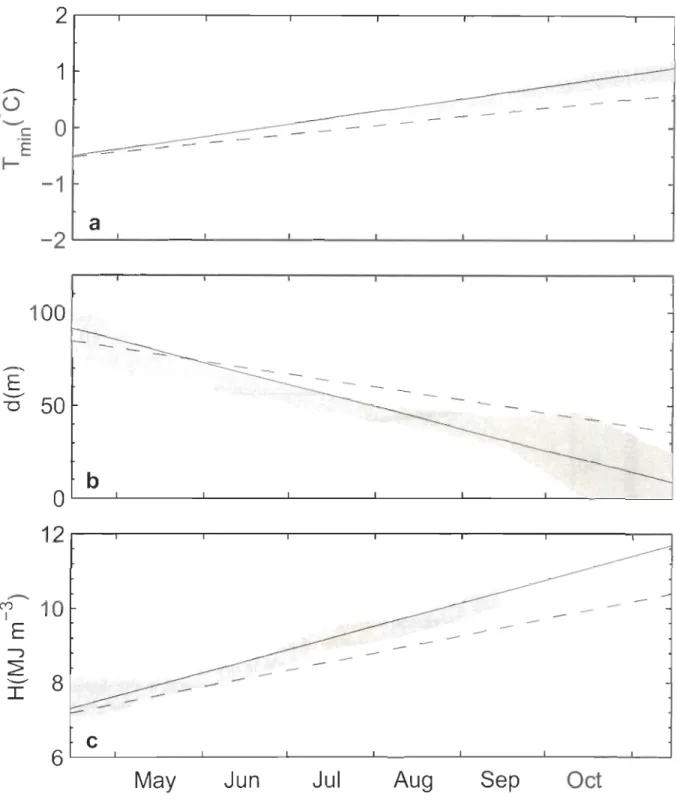
c) Modeled evolution of tempe rature using the diffusivity profile from aIl avail-able casts Ka. Figure properties are the same as Fig. 5. . . . 31 7 Evolution of CIL properties. Solid lines are monthly averages over the period

1993-2010. The shaded areas are the 95% confidence interval. a) Tempera-ture of the CIL core. b) Thickness of the CIL. c) Heat content of the CIL. d) Depth of the CIL core. Thin short lines in the three first panels are the mean slopes (erosion rates) calculated in section 1.5.1. The mean slope is reported on panels with the 95% confidence intervals (see Table 1 for comparison with model results).. . . . . . . . . . . . . . . . . . . . . . . . . . . . . . . . .. 32

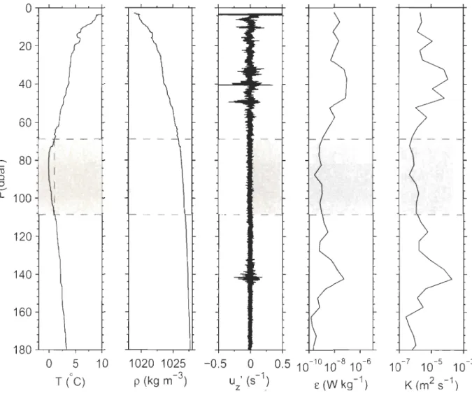
8 Interannual variability of the warming rate of the CIL core, calculated be -tween April and November for every year over the period 1993-2010. The warming rate is defined as the slope of the best linear fit of the evolution of the CIL core temperature as shown in Fig. 7a. The dashed hne is the aver-age warming rate (0.24°C mo-I) and the shaded area is the 95% confidence interval envelope (±0.04 oC mo-I ). . . . . 33 9 Typical turbulence profiler measurements, from July 21 2009. The three

left-hand panels (temperature, sea water density and vertical shear) are unfiltered profiles, i.e., sampled at 64 Hz for T and p and 512 Hz for u~. The two right-hand panels are 5-m scale TKE dissipation rate, f, and eddy diffusivity, K. The CIL has been highlighted in first panel and its depth is reported on aU panels as shaded areas. . . . . . . . . . . . . . . . . . . . . . . . . 34 10 Mean quantities from aIl 892 VMP casts for 2009-2010 (dark gray, solid

lines). a) Mean dissipation rate ofturbulent kinetic energy. b) Mean buoyancy frequency squared. c) Mean eddy diffusivity coefficient. The gray shades indicate 95% confidence intervals. Mean quantities for casts taken at

mid-channel (420) are also presented (light-gray, dashed-lines) .. . .. .. . . . 35

Il Details of the evolution of monthly mean temperature profiles for observa-tions and simulaobserva-tions. The observed 95% confidence intervals ofthe observed mean temperature profile (shaded area) is compared to two simulations done with respectively the average observed diffusivity at mid-channel Ki (dashed lines) and from aU available casts along the section Ka (solid tines). .. . .. 36 12 Comparison between observed and modeled CIL erosion rates: a) core

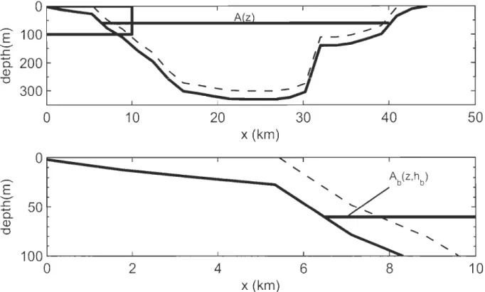
tem-perature, b) thickness and c) heat content. 95% confidence interval of the observations (1993-2010) are presented, together with the 1inear best fits of the monthly means from the model when forced respectively with Ki (dashed lines) and Ka (solid lines). AU slopes are provided in Table 1. . . . . . . . . . 37 13 Details of the geometric scaling used to calculate the "apparent" eddy

diffu-sivity (Eq. 1.5). (upper panel) Bathymetrie section of the estuary at Rimouski station (see Fig. 2, red line). (lower panel) Enlargement of the rectangle in the upper panel. For both panels, x is the distance from the South shore. The dashed tine corresponds to the upper limit of the bottom boundary layer of height hb (not to scale for emphasis). A(z) is the channel width at depth z and A/J(z, hb) is the width of A(z) within the boundary layer. . . . . . . . . . . . . 38 14 AlI dissipation rate profiles (150) that hit the bottom (gray curves) and their

mean (thick black curve). Data are presented relative to height above bot-tom (hab). The gray shaded area highlights the visuaUy-inferred 10-m thick bottom boundary layer. . . . . . . . . . . . . . . . . . . . . . . . . . . . .. 39

regions are where the CIL never reached the seabed.. . . . . . . . . . . . .. 40 16 Bathymetry of the Gulf of St. Lawrence (upper inset) and the Upper (USLE)

and Lower St. Lawrence Estuary (LSLE). The square box in the upper inset correspond to the LSLE where the study was realized (main figure). Isobaths 20, 120, 200 and 300 m have been added. The dashed line is the Rimouski section across the estuary. Second inset shows details of the study area on the northem portion of the transect, between isobaths 20-120 m (shown with 20 m intervals). Positions of mooring N080 (white star) and of the 322 VMP profiles used in this study (purple dots) are also presented. . . . .. . 68 17 Temperature and currents measured for the duration of the mooring

deploy-ment. (a) Predicted tide water level at Rimouski (L). (b) Evolution of the tem-perature field for this period as measured by the thermistor chain. Temper-ature was linearly interpolated between thermistors and a 25-hour low-pass filter has been applied. Solid lines are T

=

1°C contours. (c-d) Respectively the along-and cross-shore velocities measured by the ADCP over the slope. A 25-hour low-pass filter has been applied on both CUITent components. The vertical axis for the three last panels is the height above bottom (hab). . . .. 69 18 Example of a timeseries from the mooring for temperature (T), along- and

cross-shore velocities for a three-day period, 27-30 September 2011. The temperatures are lO-minute averaged and linearly interpolated between each thermistors, while the velocities are 1O-minute averaged and raw in the ver-tical (0.5 m). Thick solid lines in (a) are T

= 1°C

contours while thin lines are T

= 1.25 and 1.75°C.

High tides (dashed lines) and low tides (dashed-dot lines) are also identified in aIl panels for reference. . . . 70 19 Mooring conditions relative to the M2 tide cycle. AIl fields have been

aver-aged in 15-minute classes relative to the high tide. The vertical axis is the height above bottom (hab). (a) Temperature field, with isotherms 1°C and 1.3°C (black lines) added for visual reference. (b) and (c), along-and cross-shore velocities, with 0.5 m vertical bins. (d) Base-lO log of the mean shear S 2. Note that panel a spans 50 m on the vertical while others span only 25 m. Left side panels in bcd are the time-averaged profiles. . . . . . . . . . . . .. 71

20 Power spectrum density (PSD) for temperature, cross-shore (u) and along-shore (v) velocities, vertically-averaged over the depth range 0-10m (a) and

10-20 m (b) above the seabed. (c-d) Power spectrum density for the total shear (S2), along-shore

(S~ =

(~~)2)

and cross-shore shear

(S~ =

(~J2)

for the same depth ranges. The frequency is in cycle per day (cpd). Tidal Har-monies M2' M4 ,M6 and Ms have been added for reference (vertical dashed lines). The choice of the window used for PSD ca1culations (Hanning win-dow of ~2.2 days) makes the inertial frequency

f

hard to distinguish from M₂ . . . 72

21 Predicted isothenTIS displacements for a mode-2 Poincaré internaI tide (Eq. 2.9) at 4 different phases of the M

_z

tide cycle, i.e., cp

=

0, ~, Tf and

3

;

respectively (see Fig. 22). Velocity vectors for the cross-section are also added for refer-ence (v and w from Eq. 2.5). Vectors are scaled according to figure horizontal and vertical axes. (a,c) maximum dis placement, minimum velocity. (b,d) minimum displacement, maximum velocity. The bottom topography of the Rimouski section (dashed lines) with the position of the mooring N080 (ver-tical line with circles representing thermistors) are also added. The x-axis is the distance from the south shore near the city of Rimouski. . . . 73 22 Predicted temperature (T), along-(u) and cross-shore (v) velocities evolution

during a M2 tide cycle for an idealized mode-2 Poincaré internaI tide (Equa-tions 2.5 and 2.9) for approximate mooring location (y

=

33.9 km) and its depth span. For better comparison with Figure 19, the left-hand si de vertical axis is :*

= Zo

- z, where Zo

=

83 m is the total depth at mooring location. The horizontal axis also staIts at cp

=

~ instead cp

=

0 for the same reason. The water colurnn depth

z

is provided as the right-hand vertical axis of the figure. Isotherms T

=

1°C and T

= 1.3°C

have also been added in panel a (black lines). . . . 74 23 Turbulence versus water colurnn stability parameters as a function of time

and depth (m) in the proximity of the mooring on September 22, 2011, mea-sured from a drifting boat (repositioned at 16:13). (a) Dissipation rate of turbulent kinetic energy (E). (b) Background buoyancy frequency squared in 4-m bins (N2). (c) Background shear squared in 4-m bins (S2). (d) 4-m sc ale Richardson number (R;). Black lines in ail panels indicate isopycnals. Ma-genta lines in panels a and b indicate regions near the bottom where lo > KZ (see Section 2.5.3). . . . . . . . . . . . . . . . . . . . . . . . . . . . . . . . 75

when considering only flood (dashed) and ebb (dot-dashed) are also pre -sented. (a) Velocity profiles U

=

Vu

2

+

v

2 from the ADCP deployed out-board, corresponding to VMP casts. (b) Shear (S2, black lines) calculated with velocity profiles from outboard ADCP, and stratification (N2, gray lines) from VMP casts. (c) Richardson number (Ri

= ~~) calculated from

the ratio of mean profiles of panel b. (d) Dissipation rate of TKE when using aIl avail-able bins (thick black lines) and bins when the size of overturns is limited by the stratification, e.g., when lo < KZ (thin gray line). Aiso on this panel, the dissipation when the size of overturns is not limited by the stratification (10 > KZ, thick gray line) and the dissipation inferred from near bottom

veloc-3

ities using the log-law scaling presented in section 2.5.3 (È

= ~;, dashed-gray

line). (e) Turbulent diffusivity calculated using a constant (r

= 0.2,

black lines) and variable (Eq. 2.4, gray lines) flux parameter. Except U, averaged profiles are calculated assuming log-normal distribution. .. .. . . 76 25 Non-linear solitary waves observed with an echo-sounder. (a) Echogram at

120 kHz of the first wave (8 August 2012). (b) Echogram at 120 kHz of the second wave (25 October 2012). (c) Echogram at 120kHz of the third wave (25 October 2012), with dissipation rate of TKE (10) superimposed. (d) Mean shear measured from the outboard ADCP during the passage of the third wave. Isopycnals (1022, 1023, 1024, 1025, 1026kgm-3_{) have been} added on panels c and d, measured with the CTD on the VMP. Turquoise curves in panels band c are the internaI wave activity Ea calculated from equation 2.1. Evidence that the vertical motions of the profiler are picked up by the outboard ADCP and interfere with the internaI wave activity index is also illustrated in panel c. . . . 77 26 (a) Comparison between the area density energy (Ea, Eq.2.1, gray) and the

mooring shear S2 (black). Dashed lines correspond to 5 standard deviation above the mean value. Gray shades correspond to enlargement of panels (b) and (c). (d) Scatter plot of Ea versus S2 for 338 internaI waves (IWs) detected in (a). The solid line is the mean shear value for the mooring deployment and the dashed hne represents 5 standard deviations above the me an value. (e) Histogram of the relative distribution of the 338 detected IWs relative to the M₂ tide cycle (dark gray). The fraction of IWs that induce significant shear enhancement is also added (light gray). . . . .. . . . 78

27 Dissipation rates of turbulent kinetic energy in function of the buoyancy fre -quency squared (N?) and the shear squared (52). (a) Observations from aU 322 profiles with bins satisfying lo > KZ removed. The solid and dashed lines are respectively Ri

=

1 and Ri

=

t.

(b) Same as

a,

for the Gregg-Henyey scaling EGH (Eq. 2.lO). Note that to keep a single colorbar, panel b is satu -rated since EGH values range between [10-13 - 10-3] W kg-I. (c) Same as a, for MacKinnon and Gregg (2003) scaling EMG (Eq. 2.11). (d-e) Respectively the vertical and horizontal averages of the three panels above to highlight the effect of the buoyancy frequency and the shear on dissipation. The shaded area is the bootstrapped 95% confidence interval on observations while the dashed-gray and the dashed-black lines are the average of panel band c

re-spectively. . . . 79 28 Map and bathymetry of the Gulf of St. Lawrence (inset) and the Lower St. Lawrence

Estuary (main panel). Sampling boxes for Stations 16 to 22 and stations 24

29

30

31

32

and 25 have 50 km2 and 20 km2 respectively. Location of monitoring Sta-tion 23 is also shown. The fixed station occupied twice in September 2012 is represented by a white star. Sites of the turbulence profiles from the 2009 survey are identified with red dots. . . . . . . . . . . . . . . . . . . . . . . . 106 Nitrate concentrations for Stations 25 (left) and 23 (right). Gray dots are aU available water bottle samples from 2000-2012. Purple dots on station 25 pro-files are the observations from the two campaigns carried out at a fixed station in September 2012. Error bars represent the mean value and its 95% confi-dence interval obtained from bootstrap analysis in 10 m depth bins. Shaded profiles are fits obtained with Equation 3.4 (see section 3.3). . . . . . Nitrate concentration along the Laurentian Channel. (upper) Transect (in mmol m3

) between stations 25 to 16 identified with dashed lines (see Fig. 28). (bottom) Mean nitrate concentration for each station. . . . . . . . . . . . . . Semidiurnal timeseries (~13 hours) of temperature (upper panel), sali nit y (middle) and nitrate concentration (bottom) for a fixed station occupied on 23 September 2012 (see white star near station 25 on Fig. 28). Temperature-salinity casts are identified with dotted-lines and water sample bottles with black asterisks. The high tide was at 13:03 and the low tide at 19:03. The nearest maximum spring tide occurred on 18 September 2012. . . . . . . . . Similar to Figure 31, but for 29 September 2012. The high tide is at 18 :59 and the low tide at 12:52. The nearest maximum spring tide is on 1 October 2012.

107

108

109

nitrate concentration versus salinity for a1l4548 measurements available from aU stations. In red, measurements with salinities lower than SA

=

32 g kg-I . In magenta, measurements with salinities greater than SA

=

34.3 g kg-I . For the 1407 measurements with SA

=

[32,34.3]gkg-1 _{(black), the correlation} coefficient with a linear least square fit (thin gray line) gives R

=

0.94. (b) Salinity profiles (black) from two casts realized on 1 October 2009. In cyan, nitrate profiles inferred from Equation 3.4. The first cast was localized in the deep area seaward of the sill at 13:32 (thick tines) and the second above the siU at 18:40 (thin lines). These time references can be found on Figure 34. 111 34 Example of a sampling carried out on 1 October 2009 near Station 25. (a)

Dissipation rates ofturbulent kinetic energy (E). Isopycnals are also plotted in background for reference. Geographical position of each cast can be roughly followed with the in set Figure. The position of the two thermographs plotted in Figure 39 is also shown on the map with a blue star. (b) Temperature field linearly interpolated between casts. The thick black line is the 1 oC isotherm. Except for the shallowest portion of the sil!, the gray area for both panels is the maximum depth of the casts which is our best approximation in this rapidly changing topography since casts were performed as close as possible to the seabed (see Section 3.3). On the shallowest portion of the siU, where the maximum depth is less than 35 m, the bottom is that estimated from ADCP measurements. . . . 112 35 Same sampling as in Figure 34, but for (a) nitrate fluxes (F NOJ and (b) nitrate

concentrations. For both panels, the white portion in the upper part of the figures correspond to the portion of the water co1umn where SA < _{32 g kg- '} . 113 36 The nutrient pump in action. Echogram at 120kHz from an echosounder

mounted below a drifting boat on 29 September 2012 (see location on Fig. 28) shows how KelvinHelmholtz instabilities develop at early flood tide (14:35 -14:40). Along-shore currents u (east and north currents rotated by 52°), den-sity (0-1), gradient Richardson number (Ri) and nitrate concentrations (C_N03) are also provided. Note that density and nitrate concentration profiles have been linearly interpolated to their respective time from casts outside the limits of the figure. These allow an estimation of the instantaneous vertical nitrate flux (see text) . . . 114

37 Close-up view of the timeseries from Figure 34. The shear (52) from the ADCP recorder (upper panel) and the dissipation rates of TKE (middle) are presented. The bottom panel is an enlargement of the middle panel where nitrate fluxes are presented over the ADCP echograrn. Note that for a better visualization of Kelvin-Helmholtz billows (starting approximately at 18:00), the bottom panel is scaled differently from other panels and only one cast out of two is presented. Missing parts of the fluxes profiles correspond to the region where 5 A < 32 g kg-Jo . . . .. . . Ils 38 Buoyancy frequency squared (N2 ), dissipation rate of TKE (E), turbulent

dif-fusivity (K) and turbulent nitrate flux (F NOJ for station 23 and 25, respec-tively. The gray intervals are the 95% confidence interval on the averaged profile. . . . . . . . . . . . . . . . . . . . . . . . . . . . . . . . . . . 116 39 Spring-neap modulation of the temperature difference between the surface

and bottom for thermistors deployed near Tadoussac (blue star in Fig. 34). (a) Tide level in Tadoussac. (b) Temperature evolution for 2009, 2 m below the surface (dash-got line) and near the bottom at 37 m deep (thick line). The temperature difference is also plotted in dashed. Vertical gray bands corre-sponds approximately to spring tides, defined here as water level above 5.3 m and below 0.8 m (thin horizontallines in panel a). The period corresponding to our sampling campaign is highlighted with a darker shade.

40 Sketch of some of the processes leading to nitrate fluxes in the LSLE. The color backgrounds represent nitrate concentration on an arbitrary scale, are but based on the average transect of Figure 30 (for data within the dashed rectangle). Outside the rectangle, concentration is extrapolated to the near-est value (no concentration data available from above the sil!). InternaI tide isopleths heaving for high (panel a) and low (panel b) tides at Tadoussac are sketched with thin gray lines for an internaI tide of vertical mode-2 with a wavelength of 60 km. Turbulent sill processes are also expected to occur driven by barotropic tidal currents. The interplay between the upwelling of nitrate-rich waters by internaI tides and the strong mixing near the sillleads to higher vertical nitrate fluxes (F) at the head of the Laurentian Channel com-pared to those at the Rimouski station (located at about 100 km downstream of the sill). Surfacing nitrate-enriched water are advected by the estuarine cir-culation, creating a subsurface nitrate concentration minimum further

down-117

climatology from AVHRR remote sensing at 1.1 km resolution. Black lines correspond to temperature contours T

=

5.35,5.55,5.65

oc.

These

corre-spond to the coldest pixels (5%, 10% and 15% in the cumulative density

function, inset) within the blue rectangle. Square box around Station 25 from Figure 28 is also shown for reference. . . . .. . . 119 42 Figure récapitulative des travaux et des résultats importants de la thèse. La

définition des variables ainsi que les incertitudes sur les valeurs présentées sont rapportés dans le tableau 4. Les dessins représentant l'échantillonnage (bouée IML4, bateau, VMP et mouillage) ont été effecutés par Eveline Ross-phaneuf. . . . .. . . .. . 122 43 Comparaison entre observations et modèle pour l'érosion de la couche

in-termédiaire froide entre avril et novembre. Panneau du haut : climatologie 1993-2010 des température à la station Rimouski (adapté de Cyr et al., 2011). Panneau du bas: moyenne de l'évolution des températures modélisées par un modèle régional à 5 km de résolution (Saucier et al., 2003) entre 1997 et 2007 pour le point de grille correspondant à la station Rimouski (données fournies par Simon Senneville). . . . .. .. 124

44 Domaine spectrale du cisaillement. (à gauche) Spectres empiriques de Nas-myth (1970) (en noir) pour différentes valeur du taux de dissipation (E E [10-1°,10-3] W kg-I ). Ces spectres sont calculés selon une fonction analy-tique présentée en annexe de Wolk et al. (2002). La ligne noire tiretée montre la portion du spectre qui croit proportionellement à kl/3 selon la théorie de Kolmogorov (1941). La portion ombragée foncée contient les échelles où se produit la dissipation visqueuse, c-à-d, les nombres d'onde plus grands que le nombre d'onde de Kolmogorov (ks)' La portion qui n'est pas ombragée correspond à la portion des spectres qui contiennent 90% de la variance en dehors de le dissipation visqueuse. Les lignes tiretées majenta délimitent l'intervalle 10-3 ~

t

~ 10-1• Les spectres du cisaillement pour trois bins verticaux choisis pour un profil datant du 22 septembre 2011 à 14h54 sont aussi présentés. Les intervalles verticaux choisis pour ces bins sont respec-tivement 6-7 m,54-55 m et 72-73 m pour les spectres rouge, vert et bleu (voir profil du cisaillement sur le panneau de droite). La portion de ces spectres en traits pleins indique la portion sur laquelle chaque spectre a été intégré. La valeur de epsilon calculée et Je pourcentage de la variance perdue (entre parenthèses) sont indiqués sous chacun de ces spectres. Les spectres de Nas-myth correspondant aux trois valeurs de epsilon calculées sont montrés en traits tiretés fins de couleur correspondante aux spectres bruts. Le panneau de gauche est largement inspiré de la figure 13 de Wolk et al. (2002). 147

45 Illustration de l'algorithme itératif permettant d'obtenir E par intégration spec

-trale. En noir: le spectre du cisaillement correspondant à celui en rouge de la figure 44. En rouge: les limites d'intégrations obtenues au points 2.2 de l'algorithme présenté ci-dessus. En vert, le spectre de Nasmyth correspon-dant à t2 et calculé en 2.5.2. Les valeurs EO, El et t2 après la mise à jour du point 2.6 sont présentées sur chaque panneau. Chaque panneau corre-spond à une itération identifiée dans le titre (ex: Ll=l; L2=1 et L3=2 sig-nifie première itération des boucles 1 et 2 et deuxième itération de la boucle 3). Seulement les deuxièmes itérations de la boucle 3 sont présentées. Les quatres premiers panneaux proviennent de la première itération de la boucle 1 alors qu'un seul panneau pour les itérations deux et trois de cette boucle est présenté ensuite (aucun panneau n'est présenté pour la quatrième itération de la boucle 1, l'algorithme ayant déjà convergé). . . . 151 46 Similaire à la figure 45, mais pour le spectre en vert de la figure 44. 152

Observations

in situ

de turbulence: contexte historique et scientifique

Les mesures de la turbulence dans J'océan ont commencé dans les années 1950 à partir

de profileurs horizontaux (Stewart et Grant, 1999), mais la discipline n'a vraiment connu son essort qu'à partir des travaux de Osborn (1974) et de l'apparition de sondes (shear probes) capables de mesurer le cisaillement à la micro-échelle, c'est-à-dire l'échelle du centimètre. Ces sondes, insensibles aux changements de température dans la colonne d'eau contraire-ment à leurs prédécesseurs (des anémomètres à fil chaud), ont ouvert la voie à l'utilisation de profileurs verticaux de turbulence, beaucoup plus faciles à déployer que des profileurs horizontaux (voir Lueck et al., 2002, pour une revue historique du sujet). Conforté par cette certaine démocratisation des techniques de mesure de la turbulence dans l'océan, le champ de recherche est toujours aujourd'hui en pleine ébulition.

L'intérêt grandissant pour l'étude des mécanismes responsables de la turbulence et du mélange est d'autant plus important que ceux-ci ne sont que très peu ou mal représentés dans les modèles numériques actuels (Umlauf et Burchard, 2005). Ceci s'explique par le fait que les échelles temporelles et spatiales contenant l'énergie d'où provient la turbulence sont

réparties sur plusieurs ordres de grandeur. En modélisation, les dimensions des grilles de cal-cul et le pas de temps des modèles posent des limitations spatio-temporelles à la résolution des plus petites échelles, c'est -à-dire les échelles où cette énergie est libérée par mélange turbulent. Les modélisateurs contournent généralement ce problème en développant des pa-ramétrisations qui servent à prendre en compte la turbulence et le mélange qui n'est pas explicitement résolu par les modèles. La stratégie à adopter pour développer de telles pa-ramétrisations consiste à relier les processus turbulents non résolus (ex: tourbillons, ondes internes, etc.) à ceux· qui le sont (ex: cisaillement des courants moyens). La mise au point de telles paramétrisations demande par contre une bonne connaissance des mécanismes qui

génèrent la turbulence.

L'intérêt pour de telles observations est d'autant plus important considérant que certains milieux comme le Saint-Laurent sont encore presque vierges d'observations de la turbulence. Le potentiel de collaboration avec les autres disciplines de l'océanographie est également considérable dans de telles circonstances. Panni les types d'études possibles, notons par exemple les flux verticaux d'éléments nutritifs, d'oxygène ou autres éléments biochimiques (Lewis et al., 1986; Rippeth et al., 2009; Bourgault et al., 2011, 2012; Williams et al., 2013), les blooms phytoplanctoniques (Huisman et al., 1999; Ghosal et Mandre, 2003; Taylor et Fer-rari, 20 L L), les couches minces phytoplanctoniques (Durham et Stocker, 2012) ou la resus -pension de sédiments (Bogucki et al., 1997; Hosegood, 2004; Bourgault et al., 2014). Toutes ces études sont basées sur des observations in situ ou numériques du mélange turbulent.

C'est donc dans ce contexte que ce sont déroulés les travaux de doctorat, c'est-à-dire celui de l'étude d'une discipline qui jouit d'un certain engouement en océanographie étant donné que très peu de choses sont actuellement connues de la turbulence dans certains mi-lieux. La toile de fond pour cette thèse est le golfe et l'estuaire maritime du Saint-Laurent où ont été effectuées les sorties de terrain (Figure 1). Dans les prochaines pages, nous ver-rons comment la turbulence participe à l'érosion de la couche intermédiaire froide du Sainl-Laurent et à la remise en suspension d'éléments nutritifs dans les eaux de surface.

Mélange en milieu côtier et couches intermédiaires froides

Il est généralement admis que le vent et les marées sont les seuls mécanismes capables de fournir l'énergie de mélange nécessaire au maintient de l'équilibre dynamique de l'océan (Munk et Wunsch, 1998; Wunsch, 2000; Wunsch et Ferrari, 2004). Alors que le vent fournit l'énergie à un taux d'environ 1 TW, les marées générées par les mouvements astronomiques fournissent l'énergie à un taux de 3.7 TW et est le mécanisme le plus probable pour fournir le mélange nécessaire à l'océan profond. Bien qu'une partie de l'énergie des marées soit

tete du

- -~henal Laurentien o

i lelPfondeur à!C*J 300

48°~~oW""~====~"".c=====69~OW""~====~~""=====6~8°~W""-=====~""-=====6~70W Longitude

FIGURE 1: Carte bathymétrique du golfe (encadré) et de l'estuaire maritime du Saint-Laurent

transférée sous forme d'ondes internes pour ensuite être dissipée dans l'océan profond, la majeure partie de celle-ci (60-70%) est dissipée dans les océans côtiers étant donné leur plus faible profondeur et leur topographie complexe (Egbert et Ray, 2000; Rippeth, 2005). Malgré

le fait que les océans côtiers occupent une petite fraction de la surface totale occupée par les

océans (~7%), ils contrôlent entre 15-30% de la production primaire à l'échelle planétaire et jouent par le fait même un rôle majeur dans la séquestration du carbone dans les océans (20-50%) (p.-ex., Tsunogai et al., 1999; Muller-Karger, 2005; Rippeth, 2005). Quantifier les mécanismes de mélange responsables de la cascade d'énergie entre les mouvements des marées et la dissipation dans les océans côtiers est donc crucial pour notre compréhension du

cycle du carbone et de ses effets sur le climat planétaire. Cette étude vise donc l'avancement

des connaissances en ce qui à trait au mélange turbulent dans ces environnements dynamiques et complexes.

D'un autre point de vue, les couches intermédiaires froides (CIF) sont des structures estivales présentes dans plusieurs bassins subarctiques. On les trouve par exemple dans les mers Noire (Tuzhilkin, 2008), Baltique (Chubarenko et Demchenko, 2010), de Bering (Kos

-tianoy et al., 2004) et d'Okhotsk (Rogachev et al., 2000), dans le golfe du Saint-Laurent (Banks, 1966) et dans l'océan Atlantique près des côtes de Terre-Neuve (Petrie et al., 1988).

Ces masses d'eau sont généralement formées durant la saison hivernale en tant que couche froide mélangée de surface. La couche de surface devient une CIF lorsqu'emprisonnée entre

une couche profonde d'origine océanique et une nouvelle couche mélangée de surface qui

apparaît généralement au printemps suite à la fonte des glaces, à l'augmentation du débit des

rivières et au réchauffement de la température de l'air. À leur fonnation, ces masses d'eau

possèdent généralement les propriétés de la couche mélangée hivernale de surface,

c'est-à-dire, sont froides et généralement riches en oxygène et en nutriments (Gilbert et Pettigrew, 1997; Gregg et Yakushev, 2005; Galbraith, 2006; Smith et al., 2006a). Par leur température,

les CIFs contrôlent donc une partie importante de l'état et du climat des bassins côtiers sub-arctiques et leur rôle est aussi de première importance pour l'écologie marine (Ottersen et al.,

est disponible quant à leur évolution estivale et à la dégradation progressive de leurs propriétés (volume, minimum de température et contenu de chaleur). Dans les pages qui suivent, le terme érosion réfère à cette évolution par mélange de la CIF à la suite de sa regénération hivernale (qui a lieu généralement de décembre à mars). Dans les bassins où la stratification est dominée par les gradients de salinité, ces couches ont un comportement passif, c'est-à-dire qu'elles se mélangent sans affecter de façon considérable le champ de densité. Cette propriété passive nous permet d'inférer le mélange turbulent nécessaire à l'érosion observée de la CIF. La comparaison entre ce mélange inféré et celui mesuré nous permet d'en apprendre un peu plus sur la répartition spatiale de la turbulence.

Le cas du Saint-Laurent

Le golfe du Saint-Laurent est un bassin d'environ 236000 km2 dont fait partie l'es-tuaire maritime (~ 9000 km2_{) qui correspond à la partie située approximativement entre} Ta-doussac et Pointe-des-Monts (Figure 1). Il est ouvert sur l'océan Atlantique via les détroits de Cabot et de Belle Isle, et reçoit son principal apport d'eau douce du fleuve Saint-Laurent. Sa bathymétrie est constituée, entre autres, de chenaux, dont le principal, le chenal Lauren-tien, s'étend sur plus de 1000 km, entre la pente continentale et sa tête près de Tadoussac (Figure 1). Ce chenal profond (>290 m) se termine alors abruptement à un seuil, où la ba-thymétrie remonte rapidement de 325 m à environ 50 m en moins de 15 km.

Les masses d'eau évoluent de façon similaire à celles décrites précédemment pour les régions subarctiques, c'est-à-dire, passant d'un système à deux couches pendant l'hiver à un système à trois couches pendant le reste de l'année (p. ex. Koutitonsky et Bugden, 1991). La CIF du golfe est caractérisée par des eaux avoisinant le point de congélation et des salinités de 32 - 33 psu. Pendant les mois d'été, la CIF existe dans le golfe sous une couche de surface mélangée (environ 0 - 50 m) et au dessus d'une couche plus chaude (1 à <8 OC) et plus salée

(> 33 psu) à des profondeurs supérieures à 150 m. Le renouvellement de la CIF s'effectue au

cours de l' hiver alors que la couche mélangée de surface s'approfondie suite au refroidisse

-ment de l'air, au mélange induit par les tempêtes de vent et, en moindre importance, suite au

rejet de saumure lié à la formation de glace de mer (Galbraith, 2006; Smith et al., 2006a).

La CIF n'est toutefois pas seulement formée localement sur l'ensemble du golfe, puis -qu'une portion de celle-ci, variable d'une année à l'autre, provient d'une intrusion d'eau du

plateau du Labrador via le détroit de Belle Isle (e.g., Lauzier et Bailey, 1957; Banks, 1966; Petrie et aL, 1988; Galbraith, 2006; Smith et al., 2006a). De plus, pour la portion du golfe correspondant à peu près à l'estuaire maritime, la trop grande stratification liée à la décharge d'eau douce du fleuve empêche la fOTInation de la CIF (Ingram, 1979b; Galbraith, 2006;

Smith et aL, 2006b). La CIF qui s'y trouve provient donc de l'advection vers l'amont de la CIF formée dans le reste du golfe. La présence de la CIF, en plus d'affecter la distribution de

température de la colonne d'eau, influence la circulation et le climat dans le golfe du Saint-Laurent (Saucier et aL, 2003). Son rôle et sa variabilité interannuelle est aussi de première

importance pour des espèces visées par les pêches commerciales telles que le crabe des neiges

ou la morue atlantique (Lovrich et aL, 1995; Dionne et al., 2003; Tamdrari et al., 2012).

Dien que la CIF soit très fréquenunent mentioIlnée ùans la liLLéraLure sur le

Saint-Laurent (voir Gilbert et Pettigrew, 1997; Smith et al., 2006a, pour un survol historique), sa

définition varie d'un auteur à l'autre. Par exemple, Lauzier et Bailey (1957) ont utilisé l'iso

-theTIne T

=

0 oC comme la limite supérieure de température pour la CIF. D'autres auteurs ont préféré des définitions différentes, comme par exemple T < 1.5 oC (Banks, 1966; Bugden et al., 1982), T < 3 oC (Gilbert et Pettigrew, 1997; Smith, 2005) ou plus récemment T < 1 oC

(p.-ex. Galbraith et al., 2013). Comme la recherche présentée s'intéresse à la CIF durant les mois d'avril à novembre, cette dernière définition a été retenue puisque l'isotherme T

=

1 oC

est approximativement le minimum de température restant à la fin de notre période d'étude,

c'est-à-dire, lorsque la CIF disparait lors de sa fusion avec la couche hivernale de surface.

nal Laurentien, alors que la couche de surface s'écoule généralement vers l'océan et les couches profondes remontent graduellement le golfe jusqu'à l'estuaire (Koutitonsky et Bug-den, 1991). Étant donné cette circulation, la couche intermédiaire froide termine son parcours vers l'amont

à

la tête du chenal Laurentien où elle est extraite vers la surface grâce au vigou-reux mélange vertical qui est suspecté d'être présent à ce seuil (p. ex. Ingram, 1975, 1976,

1979b, 1983, 1985; Gratton et al., 1988; Saucier et Chassé, 2000), mais encore jamais mesuré avant ce doctorat. Les eaux profondes et riches en nutriments qui sont ainsi acheminées vers la surface sont ensuite entrainées vers l'aval par la circulation estuarienne. Cette extraction de la CIF à la tête du chenal Laurentien modifie donc de façon considérable les températures de surface le long de l'estuaire avec des effets sur le climat local. L'apport continuel de nu-triments à la tête du chenal Laurentien soutient aussi une forte production primaire tout au long de l'été dans l'estuaire maritime (Levasseur et al., 1984; Therriault et Levasseur, 1985; Pl ourde et al., 2001).

De récentes études ont permis à la fois une meilleure compréhension des mécanismes de formation et d'évolution de la CIF durant l'hiver (Galbraith, 2006; Smith et al., 2006a,b), de même que sa réponse à la variation des forçages par le vent et par le débit du fleuve (Saucier et al., 2009). De plus, une meilleure description de sa variabilité intra-annuelle et interannuelle a été proposée (Gilbert et Pettigrew, 1997). Cette étude, utilisant 47 ans de données provenant de 5 régions du golfe (l'estuaire, le détroit de Cabot et les régions nord-est, nord-ouest et centre du golfe) consistait en une étude plus complète que celle menée par Banks (1966). Alors que celui-ci proposa que le coeur de la CIF (minimum de température rencontré à l'intérieur de celle-ci) se réchauffait à un rythme de 0.2 oC par mois entre avril et novembre, étude basée sur 10 ans de données provenant de 3 régions du golfe (centre du golfe, détroit de Cabot et détroit d'Honguedo), Gilbert et Pettigrew (1997) proposaient qu'au contraire le coeur se réchauffait de façon différente d'une région à l'autre, augmentant de 0.08 oC à 0.30 oC par mois, respectivement pour le centre du golfe et l'estuaire.

Cependant, aucune de ces études ne quantifie le mélange turbulent responsable de cette

érosion. Cette quantification et l'identification des mécanismes d'érosion ainsi que leur lien

avec l'environnement physique est une étape clef à la fois pour la prédiction de la variation

interannuelle de la CIF et au sens plus large pour une meilleure prise en compte du mélange les modèles numériques. Ceci est doublement important pour la CIF du Saint-Laurent qu'il

s'avère que la mauvaise représentation des processus de mélange turbulent pourrait être

à

l'origine d'erreurs dans la modélisation de la formation de la CIF dans le golfe (Smith et al., 2006a).

Problématique et objectifs de la recherche

Profitant du manque de données autour de la question des processus d'érosion, les

tra-vaux de thèse visent à mieux comprendre l'érosion de la CIF et son extraction à la tête du

chenal Laurentien. Il faut comprendre ici que l'étude de la CIF est une mise en contexte plus spécifique (ou un prétexte) pour l'étude du mélange turbulent dans l'estuaire maritime du Saint-Laurent. Plus spécifiquement, les objectifs principaux de la thèse sont les suivants:

1. Identifier et quantifier les mécanismes responsables de la turbulence qui mélange la

couche intermédaire froide;

2. Quantifier le flux de nutriments qui résulte de l'extraction des couches intermédiaire et

profonde

à

la tête du chenal Laurentien.

Ces objectifs sont traités dans ce qui suit en trois objectifs spécifiques correspondants aux trois chapitres de la thèse:

- Chapitre 1 : Quantifier l'érosion estivale moyenne de la CIF et quantifier le mélange qui

s'opère dans le golfe;

Chapitre 2 : Étudier le comportement de la CIF près des bords de l'estuaire maritime et

profondes à la tête du chenal Laurentien.

Voici les résumés des trois chapitres de la thèse:

Chapitre 1 : Interior versus boundary mixing of a cold intennediate layer

Le résultat principal de cet article publié dans Journal of Geophysical Research (Cyr et al., 2011), est notre capacité à déterminer l'importance relative du mélange près des bords

(boundary mixing en anglais) sur le budget de mélange total du golfe du Saint-Laurent. Dans

cette étude, nous avons tout d'abord quantifié l'érosion de la CIF à partir de profils his

-toriques de température et de salinité. Nous avons ensuite quantifié le mélange à partir de nouveaux profils de turbulence réalisés au cours de la thèse. Nous avons déterminé qu'en -viron deux-tiers du mélange nécessaire à l'érosion de la CIF est assuré par la turbulence à l'intérieur du bassin, alors que le dernier tiers pourrait être assuré par des processus turbu

-lents qui prennent place près des bords. Contrairement aux études précédentes sur le mélange en océans côtiers qui suggèrent plutôt que la turbulence intérieure est la principale source du mélange, nous avons trouvé que le mélange aux frontières est non-négligeable dans le golfe du Saint-Laurent.

Chapitre 2 : Behavior and mixing of a cold intermediate layer near a sloping boundary

Le résultat principal de cet article soumis au journal Ocean Dynamics, est la démonstration que le comportement de la CIF près du bord nord de l'estuaire maritime est le résultat de marées internes générées une centaine de kilomètres en amont. Ce résultat à été obtenu à par

-tir du déploiement d'un mouillage à haute résolution spatio-temporelle près du bord nord de l'estuaire pendant trois semaines à l' autonme 2011. De plus, le mélange turbulent quantifié à

partir de 322 profils de turbulence révèle que les derniers 10 m de la colonne d'eau dissipent l'énergie cinétique turbulente à un taux de flOm

=

1.6 X 1O-7Wkg-l, soit un ordre de

aussi que la dissipation durant le flot est quatre fois plus grande que durant le jusant. Les contraintes sur le fond, les instabilités de cisaillement et les ondes internes sont considérés

comme mécanismes de mélange.

Chapitre

3:

Turbulent nitrate fluxes at the head afthe Laurentian channel

Dans cet article soumis

à

Journal of Geophysical Research, nous avons quantifié les

flux verticaux de nitrate à la tête du chenal Laurentien, lieu reconnu dans le Saint-Laurent

pour le vigoureux mélange turbulent qui s'y trouve. Ces flux ont été calculés à partir de

pro-fils historiques de concentration de nitrate et de nouveaux profils de turbulence issus d'une campagne de terrain effectuée en 2009. Les flux verticaux ont été comparés pour deux sta -tions, soit la limite en amont du chenal Laurentien (la tête du chenal ou station 25) et la station

Rimouski (station 23) située environ 100 km en aval. Les diffusivités turbulentes ainsi que les

flux de nitrate

à

la base de la couche du surface sont respectivement Kst.25

=

4.5(1.1,13) x

10-2 _m2 _{ç l, Kst. 23}

₌

_{4.4(2.3, 7.6)x 10-}5 _m2 _{ç l , Fst. 25}

_{= 120(23}

_{,400) mmol m-}2

d- ' et Fst. 23

=

0.21(0.l2, 0.33) nm101 m-2 d-_'. Les nombres entre parenthèse indiquant les limites de

l'inter-valle de confiance à 95% sur la moyenne. Les observations suggèrent que la combinaison entre déplacements verticaux des isopycnes et fort mélange dans les premiers 60 m de la colonne d' cau est la clé pelmettant de soutenir les impoI1ants fl ux à la station 25 (deux à

trois ordres de grandeur plus élevé que ceux de la station 23). Un calcul d'ordre de grandeur suggère aussi que bien que ce flux pourrait soutenir la majeure partie du bloom ph

ytoplanc-tonique printannier et la production estivale post-bloom dans l'estuaire maritime. Ce calcul suggère aussi que la majorité des nitrates refaisant sUlface sont consommés dans l'estuaire maritime du Saint-Laurent au lieu d'être exportés dans le golfe.

1.1 Abstract

The relative importance of interior versus boundary mixing is examined for the erosion

of the cold intermediate layer (CIL) of the Gulf of St. Lawrence. Based on 18 years of his-torical temperature profiles, the seasonal erosion of the core temperature, thickness and heat

content of the CIL are, respectively,

t

min

=

0.24 ± 0.04 oC mo-l,

d

_min

=

-11 ± 2 m mo-1 and

fi

=

0.59 ± 0.09 Ml m-3 mo-1• These erosion rates are remarkably weil reproduced with a

one-dimensional vertical diffusion model fed with turbulent diffusivities inferred from 892 microstructure casts. This suggests that the CIL is principally eroded by vertical diffusion processes. The CIL erosion is best reproduced by mean turbulent kinetic energy dissipation rate and eddy diffusivity coefficient of E :::::: 2 X 10-8 W kg-1 and K :::::: 4 X 10-5 m2 çl,

re-spectively. It is also suggested that while boundary mixing may be significant it may nOt dominate CIL erosion. Interior mixing alone accounts for about 70% of this diffusivity with

the remainder being attributed to boundary mixing. The latter result is in accordance with

recent studies that suggest that boundary mixing is not the principal mixing agent in coastal

1.2 Introduction

Cold intermediate layers (CILs) are common summerfeatures of man y subarctic coastal seas. Such water masses are found for example in the Black Sea (Tuzhilkin, 2008), the Baltic

Sea (Chubarenko and Demchenko, 20] 0), the Bering Sea (Kostianoy et al., 2004) the Sea of

Okhotsk (Rogachev et al., 2000), the Gulf of St. Lawrence (Banks, 1966) and can aIso be found in coastal oceans (Petrie et al., 1988). At formation, CILs may represent up to 45% of

the total water volume of those systems (e.g., Galbraith, 2006) and therefore largely control the state and climate of subarctic coastal systems as weIl as the marine ecology (Ottersen

et al., 2004).

The characteristics of CILs are principally governed by the properties of the surface

mixed layer formed during the previous winter (Gilbert and Pettigrew, 1997; Gregg and

Yakushev, 2005; Galbraith, 2006; Smith et al., 2006a). The CIL is formed when this surface

mixed layer becomes inslliated from the atmosphere by near-surface stratification caused by sea-ice melt, heat fluxes and increased runoff at the onset of spring. Other mechanisms such

as horizontalfintra-Iayer convection may also contribute to CIL formation (Chllbarenko and

Demchenko, 2010).

Most previous studies on CILs have focused on formation mechanisms but there is

!ittle published information about the summer deterioration of their properties by mixing processes, later recalled as erosion. One particularity of CILs is that since They lie at interme-diate depths, away from surface and bottom boundary layers, one may hypothesize that their erosion is principally governed by interior mixing processes. However, CILs also intersect the sloping bottom around Jateral boundaries where turbulent processes may be much more intense than within the interior. While the fraction of CIL volume in contact with the sloping

bottom may be small the role of boundary rnixing may still be important if turbulence is suffi

-ciently large. This is analogous to the boundary mixing hypothesis proposed by Munk (1966)

and estuaries (Bourgault and Kelley, 2003; Bourgault et al., 2008) with the hypothesis that breaking internaI waves along sloping boundaries is the main mixing agent. It has also been

proposed that boundary mixing may be the main contributor to the mixing budget of lakes

(Goudsmit et al., 1997), where wind-induced seiches are the principal driving mechanism,

and to that of coastal seas with virtually no tides su ch as the Baltic Sea (see Reissmann et al.,

2009, for a review). Other studies have however concluded that mixing in coastal seas is pre-dominantly driven by interior rather than boundary processes (e.g., MacKinnon and Gregg,

2003; Rippeth, 2005; Palmer et al., 2008).

Another interesting aspect of CILs is that they can be considered as passive tracers when

the buoyancy-driven circulation of coastal seas is principally driven by sali nit y gradients. In this case, CILs are analogous to the yearly realization of a large-scale dye release experiment. Under this hypothesis, the CIL fills uniformly the entire sea and can only be modified, or eroded, by vertical turbulent processes.

The objectives of this study are to examine whether vertical mixing alone can explain CIL erosion rates and, if so, to determine the relative importance of boundary versus in-terior mixing. To reach these objectives, we examine the erosion of the CIL in the Gulf of St. Lawrence using 18 years of historical CTD data, new turbulence measurements (892 casts) collected during summers 2009-2010 and a one-dimensional heat diffusion model. The his-torica) CTD observations are used to provide statistics on CIL erosion rates and the turbulence measurements are used to provide eddy diffusivity values used in the one-dimensional model. After assessing the model we examine the relative importance of interior versus boundary mixing by comparing the modeled CIL erosion rates with and without considering diffusiv-ity values measured near boundaries. The results are then interpreted based on a geometric scaling from which an effective eddy diffusivity is inferred and the relative contribution of boundary versus interior CIL mixing is determined.

1.3 The Gulf of St. Lawrence

The Gulf of St. Lawrence, including the estuary, is an area of about 236 000 lan2 opened to the Atlantic Ocean through Cabot Strait and the Strait of Belle Isle (Fig. 2). The bathymetry is characterized by deep channels (> 200 m), large shelves and islands. The main channel, called the Laurentian Channel, is a submarine glacial valley that runs from Tadoussac to the continental slope, past Cabot Strait (Fig. 2). The residual circulation in this channel is estuarine-like, principally driven by the freshwater discharge of the St. Lawrence River and other surrounding rivers (e.g., Koutitonsky and Bugden, 1991).

In

winter, the water column

exhibits a 2-layer structure with a 40-150 m thick surface mixed layer with temperature near the freezing point (Galbraith, 2006) overlying a warmer (1-6 OC) but saltier (> 33 psu) bottom layer of oceanic origin (roughly 150 m-bottom). The rest of the year, the water column is

characterized with three layers with the CIL sandwiched between the warmer surface and bottom layers (Koutitonsky and Bugden, 1991).

The CIL is characterized by near-freezing temperatures (T) and salinities (S) of 32 -33 psu. Although the Gulf of St. Lawrence CIL is frequently mentioned in the literature, its definition varies between authors. For instance, Lauzier and Bailey (1957) used T :::; 0 oC as their definition. Other authors have used other definitions such as T :S 1.5 oC (Banks, 1966;

Bugden et al., 1982), T :S 3 oC (Gilbert and Pettigrew, 1997; Smith, 2005) or more recently

T :::; 1 oC (Galbraith et al., 2011). Since the focus here is on the CIL erosion during ice-free months, we adopted the latter definition which approximately defines the coldest limit of what remains at the end of our study period, i.e., wh en the CIL is replenished the following

winter.

The CIL renewal occurs in winter when the surface mixed layer deepens following a combination of cold air tempe rature, wind-driven mixing and, to a lesser extent, brine rejec -tion due to sea ice formation (Galbraith, 2006). While the CIL is found throughout the Gulf, its presence at a given location may be due to horizontal advection from a remote formation

tween Tadoussac and Pointe-des-Monts is too stratified, due to important freshwater input, to allow for winter convection and CIL formation (Ingram, 1979b; Galbraith, 2006; Smith et al., 2006b).

While insights about CIL formation mechanisms were gained from previous field and modeling studies cited above, still little is known about CIL erosion mechanisms and rates. Based on 10 years of data from three regions of the Gulf (Honguedo Strait, Central Gulf and Cabot Strait), Banks (1966) found that from April to November the CIL minimum tem-perature (T min) warms, on average, by 0.2 oC mo-I . Based on a similar analysis but using 47 years of data from five regions, Gilbert and Pettigrew (1997) obtained CIL erosion rates ranging from 0.08 oC mo-I for the Central Gulf to 0.30 oC mo-I for the Estuary. This study also revisits these warming rates.

1.4 Datasets and methodology

1.4.1 CTD data

The CTO dataset was collected at a station named Rimouski and located at 48° 40' N 68° 35' W, about 25 km north of the city of Rimouski (Fig. 2). Thereafter, we will refer to this station as the interior station, i.e. a station in deep water (> 300 m) away from lateral boundaries. This dataset consists of 418 casts collected by Maurice-Lamontagne Institute staff (Fisheries and Oceans Canada, OFO) between 1993 and 2010 and obtained through the DFO Oceanographie Data Management System (Fisheries and Oceans - Canada, 20 Il). The station is typically visited once a week during ice-free months (Plourde et al., 2008) and, for the purpose of this study, only casts sampled between April and November have been selected. Temperature and salinity profiles were averaged into 1 m vertical bin size and aIl profiles of the same month have been averaged into a single monthly climatologie al profile (Fig. 3 and 4). The 95 % confidence intervals on the monthly

averaged profiles have