T
T
H
H
È
È
S
S
E
E
En vue de l'obtention du
D
D
O
O
C
C
T
T
O
O
R
R
A
A
T
T
D
D
E
E
L
L
’
’
U
U
N
N
I
I
V
V
E
E
R
R
S
S
I
I
T
T
É
É
D
D
E
E
T
T
O
O
U
U
L
L
O
O
U
U
S
S
E
E
Délivré par l'Université Toulouse III - Paul Sabatier Discipline ou spécialité : Ecologie, Biodiversité, Evolution
JURY Sergine Ponsard Roger Pradel Michael C. Runge Peter B. Pearman Emmanuelle Cam Jérôme Dupuis
Ecole doctorale : SEVAB
Unité de recherche : UMR 5174 Evolution et Diversité Biologique Directeur(s) de Thèse : Emmanuelle Cam et Jérôme Dupuis
Rapporteurs :
Roger Pradel
Michael C. Runge
Présentée et soutenue par Florent BLED Le 18 mai 2010
Titre : Tests d'hypothèses en dynamique des populations fragmentées: développement et applications de modèles d'occupation des sites
Title: Tests of hypotheses in fragmentated population dynamics: development and applications of site occupancy models
In memory of Max Bled To my goddaughter, Charlotte
Abstract – The knowledge of distribution and local abundance of organisms is a major
1
element of population studies. It has several implications in areas ranging from basic research 2
in population dynamics to more applied topics such as conservation and population 3
management. The distribution and abundance of organisms involves both physical and biotic 4
processes that vary spatially and temporally, and additionally, are typically non-linear and 5
dynamic. While a common type of data used to assess species occurrence is binary presence-6
absence data, classical approaches to the development of spatial models for binary processes 7
(i.e. "occupancy processes") present three important deficiencies. 8
9
First, they do not explicitly accommodate sampling uncertainty in the form of false 10
absences. Hierarchical modeling accounting for uncertainty in detection permits consideration 11
of this problem, but even in that case, there are problems in accounting for sampling or in 12
conditioning model on the presence of the species of interest in the area where the sampling 13
protocol is conducted. Secondly, there is an lack of spatio-temporal models of occupancy, 14
especially in the framework of hierarchical modeling. Finally, most of existing models are 15
phenomenological models and do not explicitly consider underlying ecological mechanisms. 16
However, it is obvious that when it is possible to use ecological mechanisms to describe and 17
predict site occupancy, this is an advantage. 18
19
In this thesis, I have developed spatio-temporal occupancy models for dynamical ecological 20
processes in order to respond to these limitations of actual site occupancy modeling. Such 21
models are critical for modeling the spread of important diseases by wildlife populations, the 22
spread of invasive species, and range dynamics in the presence of a changing environment. A 23
general hierarchical modeling framework is proposed for spatio-temporal dynamic occupancy 24
processes in the presence of uncertain observations. In addition to incorporation of sampling 25
uncertainty in the observations, a key component of this research is related to the incorporation 26
of scientific knowledge in the model. One of the primary goals of my research has been to 27
develop scientifically-meaningful and statistically rigorous models for spatio-temporal 28
dynamic occupancy processes in the presence of uncertainty that can be used at several 29
different geographical scales. Moreover, I wanted to propose a structure of models adaptable to 30
several topics, correcting issues that appeared in previous general occupancy models. 31
32
Simultaneously with modeling issues, three main ecological topics are addressed in this 33
thesis. The first is related to invasive species that are commonly claimed as the second threat 34
on biodiversity. In order to apply a relevant response to the potential danger associated with 1
invasions, it is essential to understand invasion mechanisms and dynamics. Focusing on the 2
propagation of an invasive species in USA (the Eurasian collared dove), I have developed a 3
general hierarchical spatio-temporal dynamic occupancy framework accommodating the 4
probabilistic automata case and generalizing it to the realistic situation in which there is 5
uncertainty in the observations. Secondly, I have focused on nesting sites in the kittiwake. Here, 6
I have proposed a model that explicitly encompasses hypotheses developed in the framework 7
of habitat selection to estimate nesting site occupancy dynamics within a cliff. Evolutionary 8
ecology provides a conceptual framework to address the relationship between individual 9
decisions and habitat features. We estimated demographic processes of site persistence (an 10
occupied site stays occupied), and colonization through two subprocesses: first colonization 11
(site creation) and recolonization (a site is colonized again after being deserted). Moreover, my 12
model incorporated local and neighboring breeding success and conspecific density in the 13
neighborhood. Finally, I have applied the work addressing the issue of conditioning on the 14
presence of the species in the area of interest and its implication for estimation of occupancy 15
rate. I have estimated the evolution of the occupancy rates of several bird species in a French 16
forest regarding of climatic changes and considering spatial heterogeneity. Our model is used 17
to study the impact of three consecutive particularly cold winters on a selected set of bird 18
species. I have focused on a limited range of factors that might influence the response of some 19
bird species to climatic changes (sedentary vs migrating species ; biogeographical origins). 20
21
Conservation efforts require the ability to understand range and occupancy dynamics as a 22
function of changes in dynamic features such as land use and climate. Such understanding will 23
permit prediction of occupancy changes that are likely to accompany future changes and 24
hopefully will permit informed attempts to mediate changes in occupancy that are viewed as 25
undesirable. I have discussed in the last part of this thesis the future ways site occupancy 26
modeling could take and that will ultimately lead to the understanding of occupancy dynamics 27
required for conservation and management. 28
Acknowledgements
First of all, I would like thank EDB laboratory and the USGS Patuxent Wildlife Research 1
center where I have conducted my research. I would also like to thank the international 2
relationships service of the Université of Toulouse 3 and the "Conseil Général du Finistère" for 3
their funding that made possible my trips to the USA. 4
I would like to thank Brigitte Crouau-Roy and the whole team of researchers of the EDB 5
laboratory for letting me works with them. 6
7
I deeply express my gratitude to Pr. Emmanuelle Cam and Jérôme Dupuis who have been 8
the directors of this PhD for all their support, help and scientific emulation they have provided 9
to me, probably not even realizing how much it was a great experience to work with them. 10
During more than three years, I have learned from them much more than just scientific 11
knowledge. 12
13
I would particularly like to thank Sergine Ponsard, Michael C. Runge, Roger Pradel and 14
Peter B. Pearman who have accepted to participate in my PhD jury. I am grateful to the 15
reviewers for their helpful comments. 16
17
I would also like to thank Sovan Lek and Claude Maranges who are the directors of the 18
Doctorate school SEVAB for their help in the submission process of this thesis. I am also 19
grateful to Dominique Galy, Dominique Pantalacci, Peggy Leroy and Marie-Martine Bègue 20
who have been of great help in the administrative tasks that I had to experience during these 21
three years. 22
23
I am grateful to Andy Royle for accepting me in the USA, for his help both scientifically 24
and personally once I have been there. I also thank him for all the interesting conversations we 25
had, and for granting me access to BBS data. I would also like to thank Bill Link, Jim Hines 26
and Jim Nichols for their comments on my work when I was over there. 27
28
I thank Marc Kéry, Béni Schmidt and Robert Dorazio for letting me attend the workshop on 29
hierarchical models in ecology in Zurich. 30
31
I am grateful to Jean-Yves Monnat for accepting me on fieldwork, for having been in my 32
PhD committee and for the experiences I had thanks to him on Cap Sizun cliffs, handling 33
kittiwakes' chicks. I am also grateful for sharing his vast knowledge, not only on the kittiwakes, 1
but also as a great naturalist, and cook. 2
I thank Jean Joachim for our interesting exchanges and for letting me know more about the bird 3
community in South France, and for letting me use his data. 4
I wish to thank all the people who have at one time or the other participated to the kittiwake 5
survey and to the breeding bird survey that permit this work. 6
7
I would also like to thank Etienne Danchin and Philippe Heeb for the comments they gave 8
me during this thesis. 9
I am grateful to Pierrick Blanchard, Pascal Mirleau and Jean Baptiste Ferdy for having been 10
such great office colleagues. Pierrick.... Keep on doing GRS, you'll be the next Paul Hunth! 11
12
I am thanking Jean-Sébastien Pierre who has accepted to participate in my PhD committee, 13
and Denis Poinsot. Both of them opened a new area of interest in Science for me. By their 14
passions, their open-mind and their abilities to share all of these, they have significantly 15
(p<0.001) marked my journey. 16
17
I am deeply grateful to Karl Doré, Laure Simonin, Brice Maret, Laurent Kernéis, Malvina 18
Rognant-Lak and Charlotte Veyssière. You have been here during the best and the most 19
difficult times and I can not thank you enough for this. 20
I am thanking Lise Aubry, David Koons, Elise Zipkin, Sarah Converse, Beth Gardner, 21
Julien Martin, Adam Green and Suzie Ponce for their support, and for all the good moments 22
we had while in the USA. 23
Thanks to all the young generation of the EDB community for all the fun and activity they 24
have created in the 4R3 building and in my life: Pierre-Jean Malé, Juliane Casquet, Kyle 25
Dexter, Candida Shinn, Laetitia Buisson, Clément Tisseuil, Frank Jabot, Erwan Quéméré, 26
François Chassagne. I am also thanking Ael Kermarec, Elodie Stéphan, Eric Bard, Sébastien 27
Goumon, Masayoshi Sugimoto, Camille Ansquer, Lyndsay Aitken, Mathieu Rognant, Aurèle, 28
Gilles, Cécile, Delphine Gallou-Papin and Raphael Papin-Gallou, Adrien Chorein, Jean Calice, 29
Marine El Adouzi, Vincent Cuminetti, Cléx, Marine, Mik, the A.D.L.M. who have been part of 30
my life, and helped me to be what I am now. And thanks again for all of you termajis that help 31
make this life better! I also deeply thank Speed Burger and la Boite à Pizza for their 32
unconditional help in the healthy nutrition process that occurred during this PhD. 33
Finally, I would like to thank from all my heart my family, especially my mother, my 34
godmother, my godfather (and the 2kg Gilt-head bream), and my aunt Rachel. If you weren't 35
here, this thesis would not have been possible. You taught me how to fish instead of simply 1
giving me a 'tacot'. Thank you for this. I also thank my brother for everything we share, and I'd 2
like you to know how much I'm proud of you. I'll never forget all of you. 3
On a fluffier note, thanks to Radjah that help the life to be bouncier! 4
5
I'd like to end these acknowledgements by dedicating this thesis to my father and my 6
goddaughter. Charlotte, your smile and your incredible blue eyes are the sunrays that permit to 7
see a blue sky behind the clouds, even in Brittany. You are my sunshine and I could not love 8
you more, but I keep trying to do so for all my life. Dad, without you, I don't know where I 9
would have been. You are a model for me and I'm proud to be your son. This thesis is yours. 10
Love you... 11
SUMMARY
Acknowledgements Summary List of tables List of figures Chapter I: Introduction ………. 1Classical models in ecology and epidemiology Limits of classical models CLASSICAL ISSUES IN SITE OCCUPANCY MODELS ……….……….. 7
Detectability Spatio-temporal dimension Fitting models and mechanistic models PARTICULAR BIOLOGICAL TOPICS ADDRESSED IN THIS THESIS ……… 15
European Collared Dove: invasion process in the USA Nesting site selection by the kittiwake Occupancy rates variations under climatic changes REFERENCES ………..……….. 18
Abstracts ………..………..……… 27
Chapter II : Hierarchical modeling of an invasive spread: case of the Eurasian collared-dove Streptopelia decaocto in the USA ……… 43
INTRODUCTION ………..……….. 47
MATERIAL ………..……….. 51
THE MODEL ………..……… 52
Occupancy state model Re-colonization reparametrization Spatial structuration Observation Model Model adaptations Spatial structure Anisotropy or directional spread Observation process Bayesian analysis and implementation in WinBUGS RESULTS ………..………. 64
Spatial structure Distance Invasion spread direction Density Detectability DISCUSSION ………..……….. 65
ACKNOWLEDGEMENTS ………..……… 73
LITERATURE CITED ………..……….. 73
Chapter III : Assessing hypotheses about nesting site occupancy dynamics ……… 89
INTRODUCTION ………..………. 92
METHODS ………..……….……… 96
Data Statistical analyses: spatial neighborhood THE MODEL ………..………..… 98
Occupancy state model Re-colonization reparametrization Spatial structure Habitat selection: density, local and neighboring breeding success Conspecific attraction, density Local breeding success Neighboring breeding success Interactions among local success, neighboring success rate, and density SURVIVAL AND SITE FIDELITY IN MARKED INDIVIDUALS ……… 105
BAYESIAN ANALYSIS ………..……… 106
RESULTS ………..……….. 107
Relationship between site-specific breeding success and persistence Relationship between conspecifics presence (through density) and dynamics parameters Relationship between neighboring breeding success and dynamics parameters Interactions among covariates Owner's fidelity to site Owner's survival DISCUSSION ………..……….. 110
Relationship between site-specific success and site persistence Relationship between conspecifics presence through density and dynamics parameters Relationship between neighboring breeding success and dynamics parameters Interactions among covariates Model development and potential applications ACKNOWLEDGEMENTS ………..……… 116
LITERATURE CITED ………..……… 117
TABLES ………..………..…… 124
FIGURES ………..………..…… 127
Chapter IV : Estimating the occupancy rate of spatially rare or hard to detect species: a conditional approach ………..……… 135
INTRODUCTION ………..……… 137
THE EXPERIMENTAL PROTOCOL AND DATA DESCRIPTION ……… 138
MODELING DETECTABILITY AND OCCUPANCY ……… 139
Underlying processes. Modeling detectability Modeling occupancy. The unconditional model of MacKenzie et al.. The unconditional model of Dupuis and Joachim. The conditional model. LIKELIHOODS, IDENTIFIABILITY, ESTIMATION AND COMPUTATIONAL ISSUES. …… 143
Likelihoods.
Conditional approach. Unconditional approaches.
Estimation and computational issues
AN ILLUSTRATION ………..……… 147
Data description Prior information Results By using the conditional approach. By using an unconditional approach. DISCUSSION AND CONCLUSION………..……… 154
ACKNOWLEDGEMENTS ………..……… 156
REFERENCES ………..………. 157
COMPLEMENTARY WORK: Improving the performances of the occupancy parameter estimator in the case of a spatially rare species ………..……… 158
Chapter V : Impact of climatic variations on bird species occupancy rate in a Southern European forest ….………..………. 171
INTRODUCTION ………..……….. 174
MATERIAL & METHODS ………..……… 177
Location Data and species list MODELING ………..……….180
Underlying processes and missing data structure Notation Modeling detectability Modeling occupancy Prior information on species detectability Likelihood Estimating the occupancy rate RESULTS ………..…………..………..…… 185
DISCUSSION ………..……….. 187
Migratory status Interior vs edge forest Role of the species’ biogeographical origins ACKNOWLEDGEMENTS ………..……… 193
REFERENCES ………..………... 193
TABLES AND FIGURES ………..………...………… 200
Chapter VI : Conclusion ………..……… 211
Hierarchical modeling ………..……….……….. 212
Occupancy versus abundance: different costs for the same inferences? …………..………… 213
How to improve estimates when modeling site occupancy: incorporation of scientific insights and sampling design. ………..………..………… 215
Incorporating scientific insights Impact of A priori information Sampling design Future directions …..………..………..………….. 217
Multiple occupancy states Using information from the capture of marked animals Favoring a multi-disciplinary approach References ………...………..……….. 219
List of tables
Chapitre I. Table 1. Examples of ecological scales of organization. Each of these systems is
1
characterized by a specific 'size' parameter, 'N', that is often the quantity of interest in static 2
systems. In dynamic systems, there are analogs of survival and recruitment probabilities, 3
which are usually described by extinction and colonization parameters in metapopulation 4
and community systems. (Royle & Dorazio, 2008). ………...………… p.4 5
6
Chapter II. Table 1. Parameters used and estimated in the model …………..……… p.81
7 8
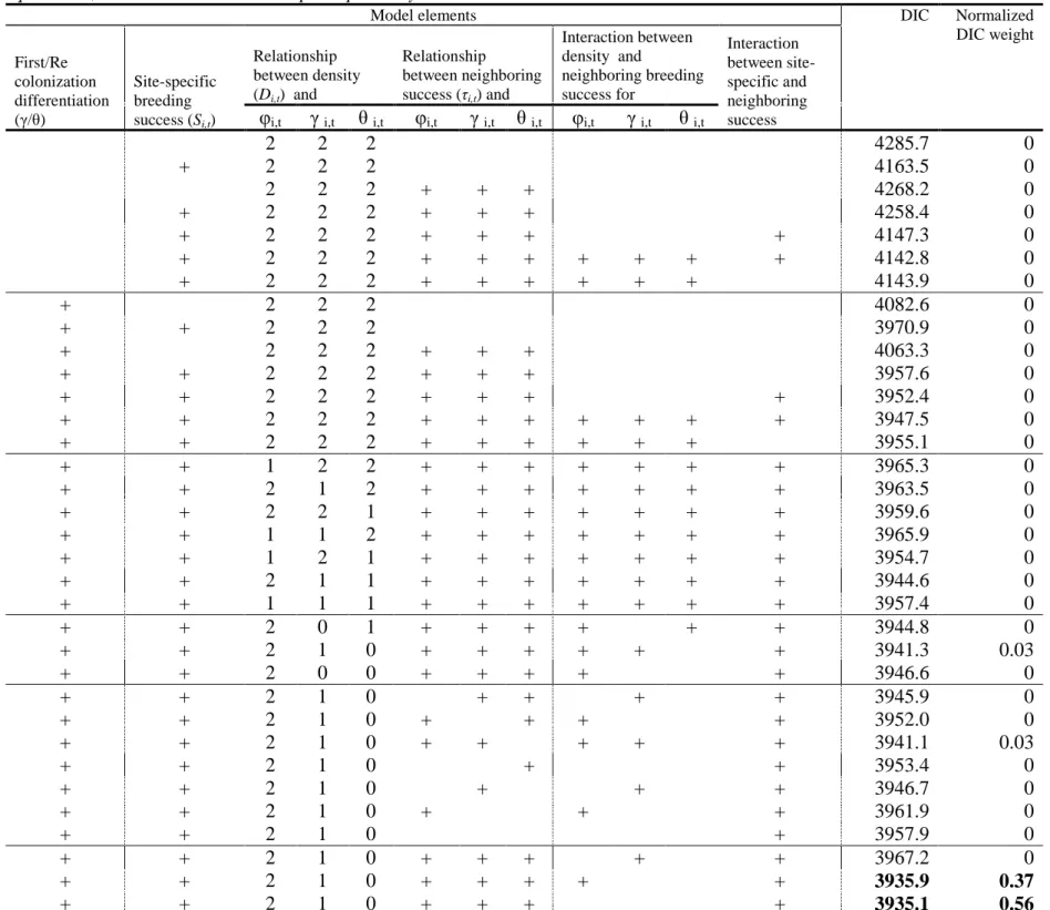
Chapter III. Table 1. Parameterization of the different models and Deviance Information
9
Criterion values. Plus sign indicates that the corresponding element is included in the model. 10
Relationship between density and dynamics parameters: ‘2’,’1’,’0’ indicate quadratic,
11
linear and no relationships respectively. Bold DIC is the selected model……… p.124
12 13
Chapter III. Table 2. Nesting site fidelity in the black-legged Kittiwake. Selection results
14
(based Akaike‘s Information Criteria) for models including breeding success S, local density 15
D, neighboring breeding success rate τ, year t and sex as covariates. Bold AIC is the selected
16
model. ……….… p.125
17 18
Chapter III. Table 3. Survival in the black-legged Kittiwake. Selection results (based
19
Akaike‘s Information Criteria) for models including breeding success S, local density D, 20
neighboring breeding success rate τ, year t and sex as covariates. Bold AIC is the selected 21
model. ……….… p.126
22 23
Chapter IV. Table 1. The data set: number of quadrats in which species s has been detected
24
(Vs) and number of visits during which species s has been detected (Ws). ……….… p.148 25
26
Chapter IV. Table 2. Prior information on detectability: coefficients of the Beta distribution
27
placed on s, prior mean and 95% credible interval of s, and coefficients of the Beta 28
distribution placed on qs. ……… p.149 29
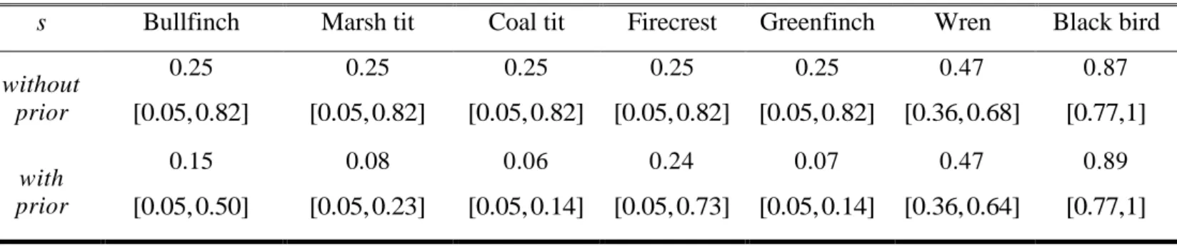
Chapter IV. Table 3. Bayesian estimations of occupancy rates under the conditional
1
approach: posterior means and 95% posterior credible intervals, with and without prior 2
information on detectability. ……….……… p. 150 3
4
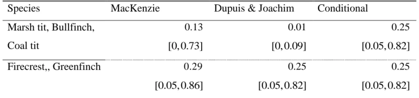
Chapter IV. Table 4. Non informative bayesian estimations of occupancy rates (posterior
5
means and 95% posterior credible intervals) yielded by the unconditional approaches of 6
MacKenzie and Dupuis & Joachim, and by the conditional approach. ………….…… p.152 7
8
Chapter IV. Supplement. Table 1. A priori 95% confidence interval for a mean a prior equal
9
to 0.3 depending a priori 'force' ρ. ……….……… p.161 10
11
Chapter V. Table 1. Data (Vs(a);Ws(a)) for 1985 and 1987 in Montech
12
forest………..………...……… p.203 13
14
Chapter V. Table 2. Migratory status and biogeographical origins of the selected species.
15
Migratory status: Sedentary (S), Migrant (M) or Partial migrant (P)……….………… p.204
16 17
Chapter V. Table 3. Prior mean and CI 95% of detection probability μsa during 1985 and 1987
18
in Montech forest……….…… p.205 19
20
Chapter V. Table 4. Posterior mean and CI 95% of sa for inner and edge regions of Montech
21
forest in 1985 and 1987. Estimates were computed using informative prior on 22
qsa………...……… p.206
23 24
Chapter V. Table 5. Posterior mean of sa and CI 95% for inner and edge regions of Montech 25
forest in 1985 and 1987. Estimates were computed using a non informative prior on qsa.
26
Only results differing from the informative approach are presented here..……… p.207
27 28
Chapter V. Table 6a. Comparison between sa estimates under unconditional (MacKenzie et 29
al., 2006) and conditional (Dupuis et al., 2010) approaches when a species is not detected,
30
for a non informative and an informative prior on qsa: case of the Green Woodpecker in
31
edge region of Montech forest in 1985. J=T=18.………...………...……… p.208 32
Chapter V. Table 6b. Comparison between sa estimates under unconditional (MacKenzie et 1
al., 2006) and conditional (Dupuis et al., 2010) approaches when a species is not detected,
2
for a non informative and an informative prior on qsa: case of the Nightingale in edge region
3
of Montech forest in 1987. J=18, T=6.…………...………...……… p.208 4
List of figures
Chapter II. Figure 1. Representation of the 2 layers of neighboring cells, used in our model in
1
estimation of local density. In black, patch 'i', in grey first layer N1 of cells, hatched:
2
second layer N2 of neighboring cells ………..………..………… p.83
3 4
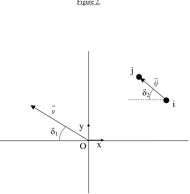
Chapter II. Figure 2. Diagrammatic representation of points and vectors used in anisotropy
5
modeling. δ1 is the angle made by the vector of invasion propagation v and abscissa. δ2 is
6
the angle made vector ij (going from site i, to site j) and abscissa. ………. p.84
7 8
Chapter II. Figure 3. Eurasian Collared-Dove site occupancy for 1996 (black area) and 2006
9
(grey area), and the corresponding estimations of probability of being colonized in 2006 10
(hatched area, p>0.5) ……….………..…….. p.85 11
12
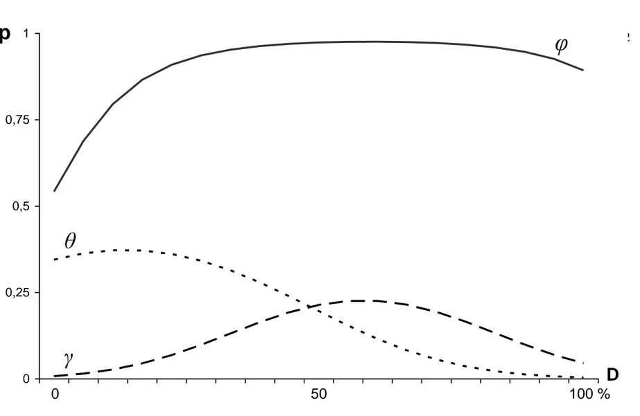
Chapter II. Figure 4. Estimates of Dynamics parameters as a function of local density D.
13
Black line is site persistence probability . Dashed line is first colonization probability .
14
Dotted line is recolonization probability . ……….……… p.86
15 16
Chapter III. Figure 1. Portion of the studied cliff in a Cap-Sizun kittiwake colony. Some
17
areas are so densely populated that nesting sites almost touch. Aggressive behavior 18
between neighbors regularly occurs. (photography by Gilles LeGuilloux) ………. p.128 19
20
Chapter III. Figure 2. . Map of the studied cliff and influence area of a nesting site. Each
21
nesting site is represented by a dot. The white dashed circle indicates the influence area of 22
one nesting site.……….……… p.129 23
Chapter III. Figure 3. Estimates of dynamics parameters as a function of local density D
1
('conspecifics presence'), for an average neighbor success rate. Black line is persistence 2
probability of a successful site Success. Grey line is persistence probability of a failed site 3
Failure
. Dashed line is first colonization probability . Dotted line is recolonization 4
probability . ……… p.130
5 6
Chapter III. Figure 4. Estimates of dynamics parameters as a function of neighbors' success
7
rate τi,t ('public information'), for an average density. Black line is persistence probability
8
of a successful site Success. Grey line is persistence probability of a failed site Failure. 9
Dashed line is first colonization probability . Dotted line is recolonization probability . 10
………...……… p.131 11
12
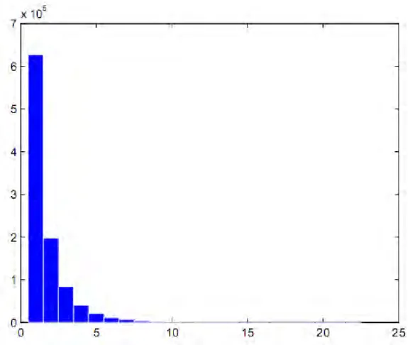
Chapter IV. Figure 1. Histogram of the MCMC sequence related to Ns =Js (L=106
13
iterations) for the marsh tit: the non informative case. ……… p.150 14
15
Chapter IV. Figure 2. Histogram of the MCMC sequence related to Ns =Js (L=106
16
iterations) for the marsh tit: the informative case. ……….………… p.151 17
18
Chapter IV. Supplement. Figure 1. Root Mean Square Error for ˆ (black line) and ˆq (grey
19
dashed line) as a function of the number of visits K, when J=100, T=100, φ* =0.1 and q* 20
=0.1. ……….…… p.162 21
22
Chapter IV. Supplement. Figure 2. Mean Square Error for ˆ as a function of the number of 23
visits K, when J=20, T=20, q*=0.1 for (a), φ*=0.6 (continuous line), (b) φ*=0.45 (dashed 24
line) and (c) φ*=0.3 (dotted line)…...……… p.162 25
26
Chapter IV. Supplement. Figure 3. Root Mean Square Error for ˆ as a function of the 27
number of visit K, when J=20, T=20, φ*=0.3 and detection probability over the whole 28
period of visit is constant and equal to 0.7. …….……… p. 163 29
Chapter IV. Supplement. Figure 4 a., b. Root Mean Square Error for ˆ (black line) and ˆq
1
(grey dashed line) as a function of the ratio r of quadrats visited, for φ*=0.3 and q*=0.1, 2
K=10 when (a) J=100 and (b) J=20. ……….…………..……… p.164
3 4
Chapter IV. Supplement. Figure 5. Root Mean Square Error for ˆ (black line) and ˆq (grey 5
dashed line) as a function of prior 'force' ρ, when J=20, T=20, K=4, φ*=0.1 and 6
q*=0.3………..……….…….……… p.164
7
Chapter IV. Supplement. Figure 6. Root Mean Square Error for ˆ using a non biased prior 8
(black line, mean prior equals 0.2) and a biased prior on φ (dotted line, mean prior equals 9
0.3) as a function of prior 'force' ρ, when J=20, T=20, K=4, φ*=0.2 and 10
q*=0.3……… p.165
11 12
Chapter V. Figure 1. European map of biogeographical region and location of Montech
13
Forest. (using data provided by the European Environmental Agency: www.eea.eu.int). 14
(Black point: Montech Forest, Cross hatch: Alpine, Diagonal simple hatch: Atlantic,
15
Ordered stipple: Continental, Horizontal simple hatch: Mediterranean). ………… p.201
16 17
Chapter V. Figure 2. Mean monthly temperatures in 1985, 1986 and 1987 (Spotted line: 1985,
18
Hachted line: 1986, solid line: 1987) compared to 1970-1984 period (maximum and
19
minimum values from this 14 year period bounded in gray). (from Joachim & Lauga, 20
1992) ……….……… p.202 21
CHAPTER I
INTRODUCTION
Ecology has been defined as "the scientific study of the interactions that determine the 1
distribution and abundance of organisms" (Krebs, 1978). The knowledge of distribution and 2
local abundance of organisms is a major element of population studies. This is the corner 3
stone in areas ranging from basic research in population dynamics (Krebs, 1978) to more 4
applied topics such as conservation and population management (Kendall, 2001 ; MacKenzie 5
et al., 2005 ; Williams et al., 2002 ; Nichols, 2004). As a result of human activities (e.g.
6
agriculture, deforestation, dam or barrage, development of highway systems), fragmentation 7
of environment in which individuals and species live has dramatically increased (Vitousek et 8
al., 1997). Individuals of mobile species often have to live in a set of subdivisions (or
9
sites/patches) of their natural habitat, and therefore may have to move from patch to patch. 10
11
It is widely recognized that many useful models of biological systems can be developed 12
from binary "presence/absence" data. Such data are relatively inexpensive and easy to obtain, 13
and may yield a maximally informative reduction of data collected under loosely organized, 14
complex or varying protocols. Indeed such data have a long history of use in ecology, 15
beginning with the investigation of spatial patterns of association between two species 16
(Forbes, 1907 ; Dice, 1945), moving to the development of theory of species distribution 17
patterns (MacArthur & Wilson, 1963, 1967 ; MacArthur, 1972), including hypotheses about 18
community assembly rules (Diamond, 1975) and nested subset community structures 19
(Patterson & Atmar, 1986 ; Patterson, 1987). These data can even be used to estimate species 20
abundance (Royle & Nichols, 2003 ; Royle et al., 2005 ; Pearce & Boyce, 2006). The last two 21
decades have seen a resurgence of interest in macroecology (Brown & Maurer, 1989 ; Brown, 22
1995 ; Rosenzweig, 1995 ; Gaston & Blackburn, 2000 ; Bell, 2001 ; Hubbell, 2001), 23
involving the study of distribution and abundance or organisms at large spatial and temporal 24
scales. The fields of biogeography and landscape ecology have also recently emerged as 25
important subdisciplines in ecology, and share many of the same goals as macroecology. 26
Conservation-oriented studies of spatio-temporal dynamics are especially timely. For 27
example, the modeling of species distribution dynamics will be useful in developing 28
predictions about distributional changes expected to accompany both land use changes and 29
active land management. Natural range expansions by a species into areas inhabited by an 30
―inferior‖ competitor species may result in range contractions of the competitor (e.g., barred 31
owl expansion into northern spotted owl range ; Anthony et al., 2006), possibly deserving 32
management actions. Investigations of species range dynamics over the last several decades 33
can provide a basis for predictions about future range changes in response to global climate 34
change. Invasive species have become a major problem throughout the world. Investigations 1
of the spatio-temporal dynamics of invasive species will permit predictions about future 2
spread as well as about the likely effectiveness of management actions designed to halt such 3
spread (e.g. Wikle, 2003 ; MacKenzie et al., 2005). 4
5
In spatial statistics, spatialization of data (e.g. "presence/absence") is commonly 6
accounted for using four types of records. (i) The spatial structure can be reflected by surface 7
recording: data are related to area delimited by borders:. This approach has long been used in 8
socioeconomics (e.g. Geary, 1954). (ii) In the case of punctual records, data refer to two 9
coordinates (x,y), and it is possible to associate surface to punctual records choosing a 10
particular point by spatial unit. (iii) It is also possible to define the spatial structure by 11
neighboring relationships. For example, two area units where records are available are 12
considered as neighbors if they share a common border. (iv) Finally, the simplest case is the 13
distance, where the spatial structure is accounted for by canonical Euclidian distance between 14
points (Chessel & Thioulouse, 2003). In all these cases of spatialized data, the site or patch 15
(i.e. points or areas where data are recorded) occupancy can be one of the variable of interest. 16
As a matter of fact, the spatial pattern of plants and animals is an important characteristic of 17
ecological communities. This is usually one of the first observations made in studying any 18
community and is one of the most fundamental properties of any group of living organism 19
(Connell, 1963). Considering a simple spatial structure, three basic types of patterns are 20
recognized in communities: random, clumped and uniform (Ludwig & Reynolds, 1988). On 21
the time scale, a patch or site is occupied or unoccupied; when an occupied patch is deserted 22
between two units of time (e.g. years or seasons), it is an extinction event. Conversely, when 23
a patch is occupied in successive sampling occasions, it is named persistence or ―survival‖ by 24
analogy with survival probability of individuals in populations. An unoccupied patch that 25
becomes occupied corresponds to an event of colonization. 26
27
These processes of occupancy dynamics will occur at different time and spatial scales, 28
whether we consider individuals, species, or even communities. When focusing on 29
individuals, ecological systems are fundamentally systems that present a hierarchy based on 30
spatial and time scale (cf. table 1, from Royle & Dorazio, 2008). 31
32 33 34
Table 1. Examples of ecological scales of organization. Each of these systems is
characterized by a specific 'size' parameter, 'N', that is often the quantity of interest in static systems. In dynamic systems, there are analogs of survival and recruitment probabilities, which are usually described by extinction and colonization parameters in metapopulation and community systems. (Royle & Dorazio, 2008)
Static system Dynamic system Population of individuals N = population size = survival
γ = recruitment Population of populations (metapopulation) N(s) = populations size spatially indexed ψ(s) = Pr(N(s)>0) 1 - = extinction γ = colonization Population of species (metacommunity) N = species richness , γ Population of communities (metacommunity) N(s), ψi(s) , γ 1
These analogies are self-evident here and they stay true when we focus on sites. For 2
example, depending on the spatial scale considered, we will always have a set of patches (e.g. 3
ponds, forests, geographical regions, continents). The only change will be in the parameters 4
of the considered ecological scale that will influence the site occupancy dynamics. At a small 5
spatial range (e.g. breeding site choice within a colony by a seabird, migration of batrachians 6
between ponds), it is a small ecological scale where site occupancy will result from 7
individual behavior of habitat selection. At a larger scale, like a country or a geographical 8
area, site occupancy may be influenced by population parameters (e.g. population size in each 9
patch). Therefore, in these conditions, site occupancy modeling can be used to address a large 10
range of apparently different biological topics. Relying on the same processes of colonization 11
and persistence, , underlying ecological mechanisms change depending on the specific 12
ecological scale. Moreover, site occupancy depends of physical and biotic processes that vary 13
both spatially and temporally (Hanski & Gilpin, 1997) and consideration of these variations 14
should be of prime interest when modeling site occupancy. 15
16
Classical models in ecology and epidemiology – At no period in the history of ecology has
17
the spatial structure of populations and communities been entirely ignored, but the part that 18
space plays in determining ecological patterns and in molding processes has been viewed 19
very differently across time (McIntosh, 1991). In the 1960s and 1970s, theoretical ecology 1
was largely focused on issues other than spatial dynamics (May, 1976), with notable 2
exceptions (Mac Arthur and Wilson, 1967), and field ecologists tended to follow suit (Hanski 3
& Simberloff, 1997). Today, space is in the forefront and is introduced in various ways into 4
all field of ecology and population biology more generally. Whether one is interested in 5
processes occurring at the level of genes, individuals, populations, or communities, spatial 6
structure is widely seen as a vital ingredient of more powerful theories, and good empirical 7
work involving space is seen as a great challenge (Kareiva, 1990). 8
In epidemiology, when studying the spatial distribution of a disease, it is recognized that 9
there are basic models which are usually assumed to apply, at least as a starting point, in the 10
analysis of case event or count data. A key role is played by the Poisson process, related point 11
process models and the Poisson distribution. When fundamental assumptions of these models 12
are not completely met, more complex models (often consisting of random effects) must be 13
invoked. (Lawson, 2006). The development of applications of models for spatial point 14
processes has gone through various phases. Many early developments took place in 15
ecological applications and, in particular, forest science (Matérn, 1986). In these applications, 16
it was often the case that relatively large realizations of points were observed (e.g. plant 17
communities or forests), mainly in a homogeneous environment. This led to the analysis of 18
models for events in homogeneous environments, and to special methods for "sparsely 19
sampled" problems, which are found particularly in ecological examples (Lawson, 2006). In 20
these early studies a number of basic models for point processes were applied. Among these 21
models the three most important in applications were complete spatial randomness (CSR), 22
spatial cluster processes and spatial inhibition processes. Diggle (2003), Ripley (1981) and 23
Cressie (1993) provide reviews of this work. 24
In the field of island biogeography, migrations rates among geographical units are 25
modeled as functions of island size, distance to a mainland, and sizes of mainland and island 26
population units (MacArthur & Wilson, 1967). Migration rates and sources of variation in 27
these rates are relevant to modeling in population genetics (e.g. island versus stepping stone 28
versus more general isolation-by distance models; Crow & Kimura, 1970). As is the case
29
with many aspects of population-dynamic modeling, human demographers were the first to 30
incorporate multiple locations into projection matrix models (Rogers, 1966, 1968, 1975, 1985, 31
1995 ; Le Bras, 1971 ; Schoen, 1988). These multiregional matrix models now are being 32
applied in animal ecology (e.g. Fahrig & Merriam, 1985 ; Lebreton & Gonzalez-Davilla, 33
1993 ; Lebreton, 1996 ; Lebreton et al., 2000). 34
1
On the basis of population dynamics parameters such as local population density, 2
population growth rate and dispersal distance, several mathematical formulations have been 3
developed to characterize and model the rate of spatial advance of spreading populations. 4
Examples include reaction–diffusion equations and their extensions (Fisher, 1937; Skellman, 5
1951; Ortega-Cejas et al., 2004) and integrodifferential equations (Van den Bosh et al., 1990, 6
1992; Kot, 1992; Neubert & Caswell, 2000). In the case of spatial disease modeling, there is a 7
wide variety of models variants available in the space-time extension. For example, semi 8
parametric models may be useful and spatial spline models are easily extended to 9
spatiotemporal situations. Autologistic models (models in which the modeling of spatially-10
distributed continuous variables is made via a conditioning on neighborhoods) can also 11
become an attractive variant for binary data as demonstrated by Besag & Tantrum (2003). 12
Modeling and inference in metapopulation models has received considerable attention 13
over the last 10 or 15 years. Much of the work has been on devising models of extinction and 14
colonization, assuming the occupancy state was perfectly observable. The Markovian state 15
model (without explicit spatial dynamics) was developed by Clark & Rosenzweig (1994). 16
Hanski (1994), Day & Possingham (1995) and others have addressed spatial dynamics. 17
Formalization of inference procedures has been addressed by Moilanen (1999) while O'Hara 18
et al. (2002) and Ter Braak & Etienne (2003) provided a Bayesian treatment of the inference
19
problem for occupancy models with temporal dynamics. These papers focus on the state 20
process model and inferences under that model assume that the state-variable can be observed 21
perfectly. 22
In metapopulation studies, when there is population turnover, it is necessary to resort to 23
modeling approaches assuming many habitat patches and local populations. Among these 24
approaches, Hanski (1994) and Hanski & Simberloff (1997) distinguished spatially implicit, 25
spatially explicit and spatially realistic approaches. Spatially implicit approaches correspond 26
to models in which all habitat patches and local populations are assumed to be equally 27
connected to each other (e.g. Levins, 1970 ; Pulliam, 1988 ; Harrison & Quinn, 1989 ; Hanski 28
& Gyllenberg, 1993). However, at some point, it is needed to incorporate specific 29
information on the spatial locations of populations. In the scope of spatially explicit 30
approaches, there are several modeling frameworks, such as cellular automata models 31
(Caswell & Etter, 1993), interacting particle systems (Durrett, 1989), and coupled map lattice 32
models (Hassell et al., 1991). Here patches as arranged as cells on a regular grid (lattice) and 33
populations are assumed to interact only with populations in the nearby "cells". The spatially 34
realistic approach includes in models the specific geometry of particular patch networks (e.g. 1
number of patches in the network, location of these patches) (Hanski & Simberloff, 1997). 2
3
Limits of classical models – Spatial models for binary processes (sometimes referred to as
4
"zero/one processes" or "presences/absence processes" or "occupancy processes") have a long 5
history in the statistics literature (e.g., for a review see Cressie, 1993). Although such 6
approaches have recently been extended to the spatio-temporal context (e.g., Zhu et al., 2005), 7
they have not focused on dynamic processes per se, and have not been used in the context of 8
data with observational uncertainty. Specifically, the classical approaches to the development 9
of such models are deficient for three reasons. First, they do not explicitly accommodate 10
sampling uncertainty in the form of false absences. That is, observed zeros (putative absence) 11
may arise because individuals are either absent from the site (a structural zero) or because the 12
species was present but went undetected in the sampling (a sampling zero). Hierarchical 13
modeling accounting for uncertainty in detection permits consideration of this problem, but 14
even in that case, there are problems in accounting for sampling errors (Sauer et al., 1994) or 15
in conditioning model on the presence of the species of interest in the area where the 16
sampling protocol is conducted. Secondly, there is a critical need for spatio-temporal models 17
of occupancy, especially in the framework of hierarchical modeling. Even if recent efforts 18
have been made to achieve a conceptual unification of models that are dynamic and models 19
with a spatial influence on the dynamics, (Zhu et al., 2005 ; Hooten & Wikle, 2008), there 20
has not been a great deal of work on statistical modeling of spatio-temporal occupancy 21
systems (Royle & Dorazio, 2008). Finally, existing models do not explicitly incorporate (i.e., 22
in the model parameterization) an explicit linkage between data and population demographic 23
process (e.g., recruitment, survival, migration, emigration). Most of the models are ―fitting 24
models‖ (i.e. phenomenological) and do not explicitly consider underlying mechanisms 25
(Bennett et al., 2001). However, it is obvious that when it is possible to use ecological 26
mechanisms to describe and predict site occupancy, this is an advantage. 27
28
Classical issues in site occupancy models
29
Detectability – Virtually all ecological sampling processes for species occurrence data admit
30
two possible events that can give rise to observed species absences: true absence, and 31
presence but nondetection. However, virtually all ecological studies of species occurrence 32
treat nondetections as true absences, leading to misleading inferences. Methods for modeling 33
and inference from such data in the presence of sampling and process uncertainty have only 1
recently become a central focus of active research and development (MacKenzie et al., 2005). 2
Nevertheless, since these methods are relatively new, they have seen little use in 3
macroecological investigations (Royle & Dorazio, 2008). More importantly, the current 4
status of these methods renders them inefficient for modeling spatially and temporally 5
dynamic processes. 6
Inferences about occupancy may be misleading when detection probability is not 7
incorporated into the methods of data analysis. Not only will naïve approaches underestimate 8
occupancy, but indices intended to reflect relative occupancy may also be biased (MacKenzie, 9
2006) and the effect of any variable of interest misidentified, particularly if detection 10
probability covaries with the factors or variables thought to affect occupancy (Gu & Swihart, 11
2004 ; MacKenzie, 2006). Inferences about the dynamic processes that drive changes in 12
occupancy may also be inaccurate (Moilanen, 2002 ; MacKenzie et al., 2003). Therefore, 13
robust inference about occupancy and related dynamics can only be made by explicitly 14
accounting for detection probability. (MacKenzie et al., 2005). 15
16
One important extension of models of occurrence or occupancy in the presence of 17
imperfect detection is to the situation in which a site's occupancy status may change through 18
time, i.e., to the situation in which the metapopulation system is "open" to local extinction 19
and colonization events. MacKenzie et al. (2003) provided a general characterization of open 20
models, and described a likelihood-based framework for inference about model parameters, 21
while Royle & Kéry (2007) provided the corresponding hierarchical formulation. An site 22
occupancy hierarchical model is described in Dupuis & Joachim (2006). The sampling design 23
required to fit such models is commonly referred to as the robust design. (Pollock 1982; 24
Kendall et al. 1995), in which replicate samples are made at each site subject to closure, and 25
sampling is repeated over time. Under these open models, the metapopulation system is 26
assumed to be closed within, but not across primary periods. Such models are referred as 27
dynamic occupancy models. 28
If we consider data obtained from repeated presence/absence (more precisely 29
detection/nondetection) surveys of i=1, 2, …, R spatial units (sites), and if we suppose that 30
each site is surveyed k=1, 2, …, K times within each of t=1, 2, …, T primary periods and that 31
each site is closed with respect to its occupancy status within but not across primary periods. 32
A typical case would be surveys repeated several times both within the breeding season of a 33
species and over several years. This situation is that for which the "robust design" (Pollock, 34
1982 ; Kendall et al., 1995 ; Williams et al., 2002 ) has been developed in conventional 1
capture-recapture applications. Let zi,t denote the true occupancy status of unit i during 2
primary period t, having possible states "occupied" (zi,t=1) or "not occupied" (zi,t=0) and yi,t 3
the observed occupancy status. One parameter of interest is the probability of site occupancy 4
(or the probability of occurrence) for period t, ψt=Pr(zi,t=1). Let φt be the probability that an 5
occupied site "survives" (i.e., remains occupied) from period t to t+1, i.e., 6
φt=Pr(zi,t+1=1|zi,t=1). In metapopulation systems, local colonization is the analog of the 7
recruitment process. Let γt be the local colonization probability from period t to t+1, i.e. 8
t=Pr(zi,t+1=1|zi,t=0). MacKenzie et al. (2003) consider a classical likelihood formulation of 9
this problem in which the model does not contain the binary state-variables (zi,t), just the 10
survival and colonization probability parameters that govern the state process, φt and γt, 11
respectively. That is, the latent indicators of occupancy are removed from the likelihood by 12
integration. However, there are situations in which one is interested in the occupancy state 13
and it is therefore important to consider a formulation that accommodates the prediction of 14
these random effects. Although not considered as such in the ecological literature, this model 15
can be naturally formulated in a state-space representation, in which the model is expressed 16
by two component processes: a submodel for the observations conditional on the unobserved 17
state process, i.e., yi,t|zi,t, and, secondly, a submodel for the un- or partially observed state 18
process involving the detection probability pi,t. 19
Therefore, we have the state process model : 20
, | , 1~ ( , ) i t i t i t
Z z Bern with i t, Pr(Zi t, 1|Zi t,1 zi t,1)zi t,1t1 (1 zi t,1)t1
21
and an observational process: yi t, Bin K( i t,, .p zi t,). 22
Despite the fact that this model and its extensions (e.g. MacKenzie et al., 2005) are a huge 23
improvement for occupancy modeling, some problems persist. The two main issues that we 24
will deal with in this thesis arise from two distinct elements: an ambiguous situation in the 25
implicit conditioning underlying this model, and a practical issue related to errors during the 26
sampling protocol. First, in the case of a closed environment (in term of geographical 27
delimitation), whether the probability that a species is detected in the sampled spatial units is 28
conditioned on the presence of this species in the whole area of studied (i.e. sampled and 29
unsampled units) is unclear. This issue is evocated in papers by Dupuis et al., and Bled et al. 30
(b.) focusing on the relationship between climatic factors and bird community state variables. 31
Specifically, conditioning (or not) on the presence of species of interest at the global scale (i.e. 32
the whole area of study containing both sampled and unsampled quadrats) is important 33
(Dupuis & Joachim, 2006). Typically, not accounting for this issue when species are detected 1
only in few quadrats (which is typically the case of spatially rare species) might have an 2
important impact on occupancy estimation. In this specific context, we have worked using an 3
informative Bayesian approach, that permitted to study how the consideration of some a 4
priori information on a parameter (e.g. detection probability) -which is not the parameter of 5
interest (e.g. occupancy probability)- might improve the precision of the estimation of the 6
quantity of interest. Secondly, many errors may arise from the data gathering, due to 7
observers' inexperience or possible misidentifications and confusion with other species for 8
example. This specific issue is addressed in the article about the propagation of an invasive 9
species in the U.S.A. 10
One consequence of detection probability lower than 1 is the presence of missing data. 11
The treatment of missing data has been an issue in statistics for some time, and it has come 12
even more to the fore in recent years. As detailed for instance in McLachlan & Peel (2000) 13
for mixture models or in Robert & Casella (1999) in a more general perspective, Markov 14
Chain Monte Carlo (MCMC) methods have been deeply instrumental in the Bayesian 15
exploration of increasingly complex missing data problems, as further shown by the 16
explosion in the number of papers devoted to specific missing data models since the early 17
1990‘s (Celeux et al., 2005). The current interest in missing data stems mostly from the 18
problems caused in surveys and census data, but the topic is actually much broader than that. 19
(Howell, 2008). Missing data create difficulties in scientific research because most data 20
analysis procedures were not designed for them. Difficulties include the computation of 21
likelihood and Bayesian estimations of quantity of interest. Missingness is usually a nuisance, 22
not the main focus of inquiry, but handling it in a principled manner raises conceptual 23
difficulties and computational challenges. Lacking resources or even a theoretical framework, 24
researchers, methodologists, and software developers resort to editing the data to lend an 25
appearance of completeness. Unfortunately, ad hoc edits may do more harm than good, 26
producing answers that are biased, inefficient (lacking in power), and unreliable. (Scafer & 27
Graham, 2002). The mechanisms (distribution patterns) of missing data are traditionally 28
divided into three classes: missing completely at random (MCAR), missing at random 29
(MAR) and missing not at random (MNAR) (Rubin, 1976). If missing data are not MCAR, 30
then there are potential problems in analyzing data as though they were, but the precise 31
outcome depends on the way in which they are missing, specifically whether data are MAR 32
or MNAR (Nakagawa & Freckleton, 2008). Therefore, when dealing with missing data, one 33
should determine in the first place what type of missing he is facing, in order to choose the 34
appropriate way of dealing with such problem (see for example Little & Rubin, 1987 ; 1
Allison, 2001 ; Schafer & Graham, 2002 or Howell, 2008 for reviews of such methods). 2
Conventional methods of handling missing data include listwise deletion, pairwise deletion, 3
dummy-variable adjustment, imputation, or maximum likelihood (Allison, 2001). A key 4
component of dealing with missing data in the context of maximum likelihood (and therefore 5
in Bayesian framework), whatever the class of distribution patterns is, is the use of data 6
augmentation. Data augmentation is a widely used algorithm particularly in Markov chain 7
Monte Carlo (MCMC) methods. The idea refers to methods for constructing sampling 8
algorithms via the introduction of unobserved data or latent variables (Tanner & Wong, 9
1987 ; van Dyk & Meng, 2001) and arises naturally in missing value problems. Here, one 10
takes advantage of the missing data structure, and this structure is used to compute a 11
complete data likelihood where the missing data are simulated conditionally on the observed 12
data. Such an approach is developed here in chapter IV in order to deal with missing data due 13
to species with a detection probability inferior to 1. Examples of applications of data 14
augmentation in a Bayesian framework include Dupuis (1995) (with the use of CMR data) 15
and Dupuis & Schwarz (2007) where computations' difficulties for Bayesian estimation, 16
hierarchical modeling, Gibbs sampling and the use of an informative a priori are also 17
considered. Dupuis & Joachim (2003) have displayed the structure of missing data in data 18
handled in the framework of site occupancy modeling, and the implementation of data 19
augmentation in this context. 20
21
Spatio-temporal dimension – The distribution and abundance of organisms involves both
22
physical and biotic processes that vary spatially and temporally, and are typically non-linear 23
and dynamic. Methods for modeling and inference from occupancy data in the presence of 24
sampling and process uncertainty have only recently become a central focus of active 25
research and development. However, the current status of these methods renders them 26
ineffective for modeling realistic spatio-temporal dynamic processes. Moreover, when the 27
three quantities of potential interest in population ecology and management (abundance, 28
occupancy and species richness) are investigated with respect to their distribution over space 29
at one point in time, inferences about dynamics processes that produce spatial patterns are 30
always very weak, as many alternative hypotheses can be invoked to explain most ecological 31
patterns (MacKenzie et al., 2005). 32
In ecological systems, concern in occupancy stems from the fundamental interest in the 1
nature and strength of relations among and within local populations. Understanding spatial 2
dynamics such as those driving the spread of invasive species (or diseases) is very important , 3
as are intrinsic population demographic processes having to do with competition, recruitment, 4
dispersal, source/sink dynamics, dynamics of species distribution and range, and other 5
macroecological concepts. Despite this interest, attention to spatio-temporal dynamical 6
models for occupancy has lagged behind, although there is a growing literature on spatial 7
models for Gaussian processes in statistics (e.g., see Banerjee et al., 2004 for a recent 8
overview) and a well-developed literature on spatial models for binary processes (e.g., see 9
Cressie, 1993 for an overview; Hoeting et al., 2000). There have been recent efforts in 10
ecology toward developing and using temporally dynamic models of occupancy (Barbraud et 11
al., 2003 ; MacKenzie et al., 2003, Eraud et al., 2007 ; Hooten et al., 2007 ; Royle & Kery,
12
2007 ; Hooten & Wikle, 2008) that accommodate both explicit concepts of population 13
dynamics as well as observation uncertainty due to sampling. Barbraud et al. (2003) dealt 14
with spatio-temporal dynamics by modeling the colonization parameter for one region as a 15
function of the local extinction parameter in a neighboring region. Other than these attempts, 16
I know of no serious work on developing models with explicit spatial or spatio-temporal 17
dynamics. 18
An interesting class of models is models that are motivated by viewing the movement (i.e., 19
dispersal) of a phenomenon (e.g. invasion of an area, range shift) from the perspective of the 20
phenomenon itself, rather than the system as a whole (i.e. directly try to model movement 21
between each specific locations rather than a global population migration). For example, an 22
exotic invasive species or a pathogenic species, in a new environment will often move from 23
areas of lower quality to areas of higher quality (quality defined in terms of many possible 24
factors, from environmental suitability to overpopulation through availability of hosts). Such 25
models have connections to cellular automata models (e.g. Wolfram, 1984). Automata are 26
most often defined in a deterministic dynamical system framework where the state of the 27
"neighborhood" of an entity (in the case of an areal unit of space, called a "cell") determines 28
the future state of the entity. Another type of automata can be formulated probabilistically, 29
where movement of an entity to its neighborhood is defined by parametric probability 30
distributions and the behavior of the system as a whole (i.e. the "automaton") -given the 31
probability rule- is not unique, but can be expressed in terms of likelihood (Lee et al., 1990). 32
A propagating automatous system defined in either manner is capable of exhibiting spatially 33
irregular wave-like behavior commonly found in natural phenomena (Hogeweg, 1988). Using 34