Science Arts & Métiers (SAM)
is an open access repository that collects the work of Arts et Métiers Institute of
Technology researchers and makes it freely available over the web where possible.
This is an author-deposited version published in: https://sam.ensam.eu
Handle ID: .http://hdl.handle.net/10985/6894
To cite this version :
Antoine DAZIN, Patrick DUPONT, Guy CAIGNAERT, Gérard BOIS - Transient behavior of a radial vaneless diffuser - In: ASME-JSME-KSME Joint Fluids Engineering Conference 2011, Japan, 2011-07-24 - ASME-JSME-KSME Joint Fluids Engineering conference 2011 - 2011
Any correspondence concerning this service should be sent to the repository Administrator : archiveouverte@ensam.eu
Proceedings of ASME-JSME-KSME Joint Fluids Engineering Conference 2011 AJK2011-FED July 24-29, 2011, Hamamatsu, Shizuoka, JAPAN
AJK2011-
06059
TRANSIENT BEHAVIOR OF A RADIAL VANELESS DIFFUSER
Antoine DAZIN Arts et Métiers ParisTech
Laboratoire de Mécanique de Lille UMR CNRS 8107
Lille, France antoine.dazin@ensam.eu
Patrick DUPONT Univ Lille Nord de France
Ecole Centrale de Lille Laboratoire de Mécanique de Lille
UMR CNRS 8107 Lille, France
Guy CAIGNAERT Arts et Métiers ParisTech
Laboratoire de Mécanique de Lille UMR CNRS 8107
Lille, France
Gérard BOIS Arts et Métiers ParisTech
Laboratoire de Mécanique de Lille UMR CNRS 8107
Lille, France
ABSTRACT
The paper refers to the behavior of a radial flow pump vaneless diffuser during a starting period. Results obtained with a 1D numerical model are compared with some new experimental data which have been obtained using 2D/3C High repetition rate PIV within the diffuser coupled with unsteady pressure measurements.
These tests have been performed on a test rig with a radial impeller matched with a vaneless diffuser. They have been made in air, on a test rig well adapted for studies on interactions between impeller and diffuser, as well as for the use of optical methods and especially Particle Image Velocimetry (PIV) as there is no volute downstream of the diffuser.
The present study refers to new experiments combining pressure measurements and 2D/3C High Speed PIV at partial flow rates within a vaneless diffuser with a large outlet radius.
Four Brüel & Kjaer condenser microphones are used for the unsteady pressure measurements. They were flush mounted on the shroud side of the diffuser wall and on the suction pipe of the pump. The sampling frequency was 2048 Hz.
For PIV measurements, the laser sheet was generated by a Darwin PIV ND:YLF Laser at three heights within the diffuser. PIV snapshots have been recorded by two identical CMOS cameras. A home made software has been used for the images treatment. The results consist in fields of 80 x 120 mm2 and 81 x 125 velocity vectors with a temporal resolution of 250
velocity maps per second. For each flow rate and each laser sheet height in the diffuser, two acquisitions of about 1500 velocity maps have been realised.
The experimental data are compared with the ones provided by a 1D transient model of the flow within the diffuser.
INTRODUCTION
The need for transient simulations of hydraulic or energy systems is becoming greater and turbomachineries are certainly the most difficult elements to model correctly during transient operations. It has been observed that the performance of machines and more particularly centrifugal pumps during transient operations can be rather different from the quasi-steady one. In the last twenty years, many studies have concerned this subject through several aspects: starting period (Tsukamoto & Ohashi [1], Saito [2], Ghelici [3], Bolpaire [4], Lefebvre and Barker[5]), stopping period (Tsukamoto et al [6]), vane opening or closure (Picavet [7]) and fluctuating rotational speed (Tsukamoto et al [8]). More recently, Tanaka and Tsukamoto [9, 10, and 11] as well as Duplaa et al [12] have explored the cavitating transient behaviour of a centrifugal pump.
Models predicting the behavior of a centrifugal impeller (Tsukamoto & Ohashi [1], Dazin et al [13]) have been proposed and are predicting correctly the performance of the pump during
transient periods. Nevertheless, there is no work focusing on the flow analysis in vaneless diffusers, whereas it is not easily predictable because the flow is not guided and thus can behave freely during the transient period.
On the other hand, the development of high speed PIV has given a performing tool to investigate flow behavior especially during transient periods.
The present paper is reporting results obtained with the help of high speed PIV in the vaneless diffuser of a radial flow pump. The experimental velocity data are compared with the results of a 1D transient model of the flow within the diffuser. NOMENCLATURE
Roman letters b diffuser width b2 impeller outlet width
c absolute velocity magnitude cf friction coefficient
cp pressure coefficient
cr radial velocity component
cu tangential velocity component
f frequency
N impeller rotation velocity p static pressure
Qdes design volume flow rate
r radial position
R1 impeller tip inlet radius
R2 impeller outlet radius
R3 diffuser inlet radius
R4 diffuser outlet radius
Re Reynolds number
Rinlet numerical domain inlet radius
Routlet numerical domain outlet radius
S mean blade thickness t time
u2 peripheral velocity at impeller outlet
Z number of impeller blades
α absolute flow angle (measured from the tangential direction)
β2 outlet blade angle (measured form the peripheral velocity) ν kinematic viscosity θ angular position ρ fluid density τ friction shear 1-EXPERIMENTAL SET-UP 11 - Pump tested and test rig
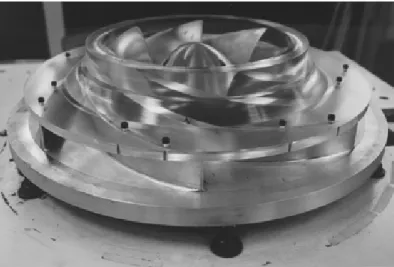
The experimental analysis was carried out on the so-called SHF impeller (fig. 1 and table 1) coupled with a vaneless diffuser.
Figure 1 : SHF impeller
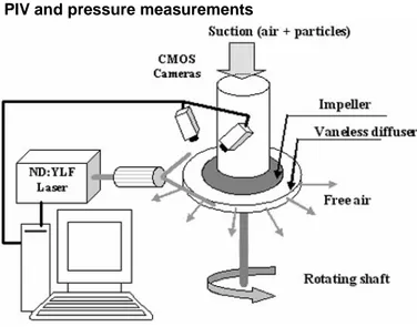
The tests were made in air with a test rig (fig. 2) developed for studying the rotor-stator interaction phenomena. Since the analysis was focused on the flow behaviour in the diffuser, no volute was used downstream the diffuser in order to guarantee the axial-symmetry of the pressure field at the pump discharge. The test rig is properly built for the application of optical analysis methods and in particular of the Particle Image Velocimetry (PIV) technique: the walls of the diffuser are transparent and the lack of volute downstream the diffuser allows large optical access for the laser sheet and the cameras. It was already used in previous studies carried out on the same impeller coupled with a short vaneless diffuser [Wuibaut et al., 14-15-16] and a vaned diffuser [Cavazzini et al, 17].
Table 1: Pump characteristics
In the present study, to favour the aeraulic inertial effects, a vaneless diffuser having a large outlet to inlet radius ratio (already used for diffuser instability studies – Dazin et al [18, 19]) was coupled with the impeller. The main geometrical
SHF impeller characteristics
R1 Impeller tip inlet radius 141.1 mm
R2 Impeller outlet radius 256.6 mm
b2 Impeller outlet width 38.5 mm
β2c Outlet blade angle (measured
from the peripheral velocity)
22.5° S Mean blade thickness 9 mm Z Number of impeller blades 7
Qdes Design flow rate at 1200 rpm 0.236 m3/s
N Impeller rotation velocity 1200 rpm Re = u2 R2/ν Reynolds number 5.52·105 Vaneless diffuser characteristics
R3
R4
b
Diffuser inlet radius Diffuser outlet radius Diffuser constant width
257.1 mm 390 mm 40 mm
characteristics of the analysed configuration together with the design operating point are reported in table 1.
12 - PIV and pressure measurements
Figure 2 Experimental set-up
The flow field inside the diffuser was studied at several flow rates by means of 2D/3C High Speed PIV and pressure transducers.
The laser illumination system consists of two independent Nd:YLF laser cavities, each of them producing about 20 mJ per pulse at a pulse frequency of 250 Hz. The pulse duration is 90 ns. A light sheet approximately 90 mm wide with a thickness of 1.5 mm was obtained at three heights in the hub to shroud direction (b/b3 = 0.25, 0.5 and 0.75 ) using conventional optical
components (2 spherical and a cylindrical lenses). The time delay between the first and the second cavity pulses was settled to 110/130 µs, depending on the flow rate. Two CMOS cameras (1680 x 930 pixel2), equipped with 50 mm lenses, were properly synchronized with the laser pulses. They were located at a distance of 480 mm from the measurement regions. The angle between the object plane and the image plane was about 45°.
As regards the seeding, incense smoke particles having a size of less than 1 µm [Cheng et al, 20] were used. These particles were
introduced near the inlet of the pump, but, as the experiments were conducted in a closed room, the whole room was seeded after few minutes of operation. The mean image particle size, estimated by image treatment, was 1.7 pixels and about 17 particles were identified in each correlation window of 32 x 32 pxl2.
The image treatment was performed by a software developed by the Laboratoire de Mecanique de Lille. The cross-correlation technique was applied to the image pairs with a correlation window size of 32*32 pixels2 and an overlapping of 50%, obtaining flow fields of 80*120mm2 and 81*125 velocity vectors. The correlation peaks were fitted with a three points Gaussian model. Concerning the stereoscopic reconstruction,
the method first proposed by Soloff et al [21] was used. A velocity map spanned nearly all the diffuser extension in the radial direction, whereas in the tangential one was covering an angular portion of about 14°. A rms uncertainty value of 1.3 pxl was obtained through the PIV analysis of a quiescent flow. Other error sources were estimated on the basis of an uncertainty analysis conducted on synthetic PIV images (Foucaut et al [22]) and the total PIV uncertainty was estimated to be less than 5% of the final velocities.
Four Brüel & Kjaer condenser microphones (Type 4135) simultaneously measured the unsteady pressure. The measurement uncertainty for these measurements was less than 1 % of the final fluctuations. The measured pressure data were acquired by a LMS Difa-Scadas system with a sampling frequency of 2048 Hz. Two of these microphones were placed flush with the diffuser shroud wall at the same radial position (r/r3=1.05) but at different angular position (∆θ=75°), whereas
the other two were located on the suction pipe of the pump, 150 mm upstream the impeller inlet. To synchronize the unsteady pressure measurements with the velocity maps, a signal was sent by the PIV system to the LMS Difa-Scadas acquisition system. Experimental measurements were acquired for the design flow rate Qdes and at 5 partial flow rates (0.26 Qdes, 0.45 Qdes, 0.56
Qdes, 0.66 Qdes and 0.75 Qdes) with a final impeller rotation
speed of 1200 rpm. The electronic speed controller which is driving the electic motor matched to the pump was programmed to impose a constant acceleration to the impeller. The maximum speed (1200 rpm) was obtained after 5 s of acceleration. The data acquisition (pressure as well as PIV measurements) were started after one quarter impeller revolution.
The results presented in this paper refer to the design flow rate, and PIV measurements obtained at mid-height.
13 - Data processing
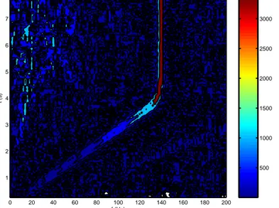
131. Impeller angular velocity determination. A Sliding Fourier Transform was applied to the pressure data obtained in the diffuser. Each Fourier transform was performed on a sliding window of 0.5 s. Thus, the frequency resolution of the Fourier Transform was 2 Hz. The results of this processing are plotted Figure 3.
0 20 40 60 80 100 120 140 160 180 200 1 2 3 4 5 6 7 f (Hz) t (s) 500 1000 1500 2000 2500 3000
Figure 3 : Pressure Sliding Fourier spectrum – microphone located in the vaneless diffuser (r/r3=1.05). The color level
gives the amplitude of the spectrum.
On this figure, dominant peaks, corresponding to the blade passing frequency can clearly be identified at each time step. The frequency, and thus the impeller velocity, corresponding to this peak is determined (Fig. 4). The precision on the rotation speed is of the order of the resolution of the spectra divided by the blade number of the impeller, that is 0.29 revolution per second.
Because of the size of the Fourier transform window, this procedure is unable to determine the velocity during the first 0.25 s. The impeller velocity, during this short period, is obtained by extrapolating the linear ramp observed in Fig. 4.
0 1 2 3 4 5 6 7 t (s) 0 100 200 300 400 500 600 700 800 900 1000 1100 1200 N (r p m )
Figure 4 : Impeller velocity time evolution.
132. PIV data processing
-0.02 0 0.02 0.04 0.06 x (m) 0.26 0.28 0.3 0.32 0.34 0.36 0.38y (m ) diffuser outlet diffuser inlet r = 0.3 m θ = θ1 θ = θ2
Fig 5 : Example of velocity map and of a line (r = 0.3 m) on which the average value of the velocity component are
performed.
Averaged values of the radial and tangential velocity components are calculated on each velocity maps (fig 5) for 100 radii from r = 280 mm to r = 379 mm (with a 1mm radial step) :
∫
=
2 1)
,
(
)
(
θ θθ
θ
d
r
c
r
c
r r (1)∫
=
2 1)
,
(
)
(
θ θθ
θ
d
r
c
r
c
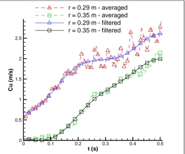
u u (2)This procedure gives consequently, at each time step and each radius, an averaged value of the radial and tangential velocity components. As can be seen on fig 6, the time evolution of these averaged velocity components are affected by a low frequency phenomenon, especially near diffuser inlet. This low frequency phenomenon is the consequence of the jet-wake flow at the outlet of the centrifugal impeller. It is noticeable on the averaged data because the angular span of a velocity map (~14°) is lower than the one of a blade passage (~52°). To get velocity components time evolutions characteristic of the transient phenomena, and not affected by the presence of the jet or wake regions, the averaged velocity
evolutions obtained by equations (1) and (2) are filtered: the data are decomposed using the Demeyere wavelet ; the fifth level approximation is used to reconstructed the filtered signal (Fig. 6). 0 0.1 0.2 0.3 0.4 0.5 t (s) 0 0.5 1 1.5 2 2.5 C u (m /s ) r = 0.29 m - averaged r = 0.35 m - averaged r = 0.29 m - filtered r = 0.35 m - filtered
Fig 6 : Averaged and filtered tangential velocity components evolution near diffuser inlet (r = 0.29 m) and outlet (r = 0.35 m)
2- NUMERICAL PROCEDURE.
To analyze the experimental results and try to predict the performance of the vaneless diffuser during transient operations, a 1D numerical model is built. The hypothesis of this model are the following :
- uncompressible flow - plane flow
- axisymetric flow
- friction shear on the walls modeled by a parabolic function of the velocity :
2
2
1
c
c
fρ
τ
=
(3)According to these hypothesis the three following equations can be written :
- Continuity equation
)
(
2
2
π
rbc
r=
π
R
inletbc
rR
inlet ( 4 ) - Moment of momentum equation :2
.
)
(
)
(
2
u f r u r uc
rc
c
r
rc
bc
t
c
br
=
−
∂
∂
+
∂
∂
(5) - Radial component of the momentum equation :0
.
1
)
(
−
2+
=
∂
∂
+
∂
∂
+
∂
∂
r f u r r rc
c
b
c
r
c
r
p
c
r
c
t
c
ρ
( 6 )The domain explored numerically is not corresponding exactly to the whole diffuser: it was limited to a region where PIV
measurements were available. The domain inlet is corresponding to the radius Rinlet = 0.28 and its outlet to the
radius Routlet = 0.379. This domain is meshed with 500 cells in
the radial direction. At each time step, experimental values of the radial and tangential velocity components at domain inlet are given as boundary conditions. The pressure at domain inlet is supposed to be equal to zero at each time step.
Then, equation (4) is easily solved: the value of the radial component of the velocity everywhere in the diffuser is automatically deduced from the one at inlet. Equation (5) is then solved with a first order scheme in space and in time. The knowledge of the previous time step and of the tangential velocity at inlet allows solving equation (5) with only one iteration at each time step. Equation (6) is then solved with the same procedure and gives the static pressure distribution in the diffuser.
The model time step is t = 0.004 s and is corresponding to the PIV one. The calculations are initialized, for the velocity component, by the experimental filtered data. For the radial velocity component, the calculations are initialized by the experimental initial value at diffuser inlet. The other values of the radial velocity are then deduced from equation (4). The initial pressure is supposed to be uniformly equal to zero in the diffuser at the beginning of the simulation.
4 - RESULTS AND DISCUSSION
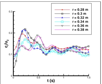
The evolution of the filtered radial and tangential velocity components scaled by the instantaneous peripheral velocity at the outlet of the impeller are plotted for different radii as a function of time in figure 7. At the beginning of the start-up, near the diffuser inlet (r = 0.28 m, fig 8) tangential velocities are of the order of the impeller peripheral velocity. This observation is consistent with previous experimental observations of a centrifugal impeller start-up [7] which had suggested that the very beginning of the start-up is characterised by a period of solid body rotation of the flow within the impeller. Concerning the other radii, at t=0, the greater the radius is, the smaller the tangential velocity component is. And, near the diffuser outlet, (r = 0.36 m and r=0.38 m on fig 8) this velocity component is equal to zero. This means that, because of inertial effects, it is not affected during the first period of the start-up. After this first period, both velocity component reach rapidly (at t=0.5 s) a nearly constant value whatever the radius is. These values are corresponding to the steady ones. Consequently, after t=0.5 s the transient effects are becoming smaller and the rest of the paper will therefore focus on the time period between 0 and 0.5s.
0 0.5 1 1.5 t (s) 0 0.1 0.2 0.3 cr /u 2 r = 0.28 m r = 0.3 m r = 0.32 m r = 0.34 m r = 0.36 m r = 0.38 m
Fig 7: Filtered radial velocity component evolution versus time. 0 0.5 1 1.5 t (s) 0 0.1 0.2 0.3 0.4 0.5 0.6 0.7 0.8 0.9 1 cu /u2 r = 0.28 m r = 0.3 m r = 0.32 m r = 0.34 m r = 0.36 m r = 0.38 m
Fig 8: filtered tangential velocity component evolution versus time
The evolution of the absolute flow angle at r = 0.28 m is plotted Fig 9. It can be seen that, during the beginning of the start-up, the flow angle at diffuser inlet is lower than the steady value. This observation is also consistent with previous experimental observations ([13]) which have shown that the flow coefficient at the beginning of the start-up of a centrifugal impeller is below the steady one because of transient effects in the system. 0 0.1 0.2 0.3 0.4 t (s) 0 1 2 3 4 5 6 7 8 9 10 11 12 13 14 α () o
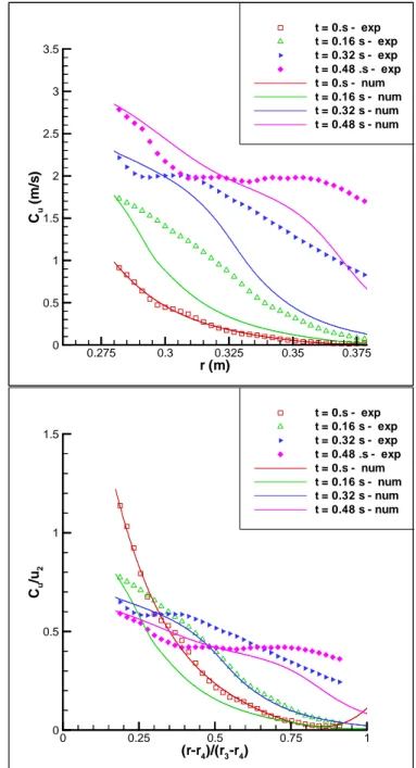
Fig 9 : evolution of the absolute flow angle at r = 0.28 m. The experimental evolution of both velocity components are compared to the results given by the numerical model during the beginning of the start-up fig 10 and 11. On Fig 10, the numerical model predicts rather correctly the evolution of this velocity component at t=0s and t=0.16s, whereas it underestimates the radial velocities at t=0.32s and t=0.48s. The numerical evolution of the radial velocity component is directly calculated by solving equation (4) which expresses the mass conservation (with a 1D hypothesis). It means that the 1D hypothesis is valid only during the very first period of the start-up. It can be supposed that this evolution is linked with the evolution of the boundary layer near the diffuser walls. During the very beginning of the start-up, the boundary layers are rather thin, and the radial velocity component is nearly constant on the whole height of the diffuser. Whereas, as these boundary layers develop, the flow rate is concentrating in a core flow between them. On top of that, the boundary layers are become thicker with the radial position. Consequently, the velocities at mid-height of the diffuser are increased with the radial position.
In Fig 11, it can be observed that the model predicts qualitatively correctly the evolution of the tangential velocity component. The greater values of this component are convected downstream by the radial velocity component at each time step. Nevertheless, it can be seen that the model is obviously underestimating the tangential velocity component whatever the time is. This underestimation is undoubtedly linked with the underestimation of the radial velocity component, and therefore by the underestimation of the second term of the left hand side of equation (5) (the convective term).
0.275 0.3 0.325 0.35 0.375 r (m) 0 0.25 0.5 0.75 1 1.25 1.5 1.75 Cr (m /s ) t = 0.s - exp t = 0.16.s - exp t = 0.32 s - exp t = 0.48 .s - exp t = 0.s - num t = 0.16 s - num t = 0.32 s - num t = 0.48 s - num 0 0.25 0.5 0.75 1 (r - r4)/(r3- r4) 0 0.1 0.2 0.3 0.4 Cr / u2 t = 0.s - exp t = 0.16.s - exp t = 0.32 s - exp t = 0.48 .s - exp t = 0.s - num t = 0.16 s - num t = 0.32 s - num t = 0.48 s - num
Fig 10: Comparison of the experimental and numerical radial velocity component. 0.275 0.3 0.325 0.35 0.375 r (m) 0 0.5 1 1.5 2 2.5 3 3.5 Cu (m /s ) t = 0.s - exp t = 0.16 s - exp t = 0.32 s - exp t = 0.48 .s - exp t = 0.s - num t = 0.16 s - num t = 0.32 s - num t = 0.48 s - num 0 0.25 0.5 0.75 1 (r-r4)/(r3-r4) 0 0.5 1 1.5 Cu /u2 t = 0.s - exp t = 0.16 s - exp t = 0.32 s - exp t = 0.48 .s - exp t = 0.s - num t = 0.16 s - num t = 0.32 s - num t = 0.48 s - num
Fig 11 : Comparison of the experimental and numerical tangential velocity component.
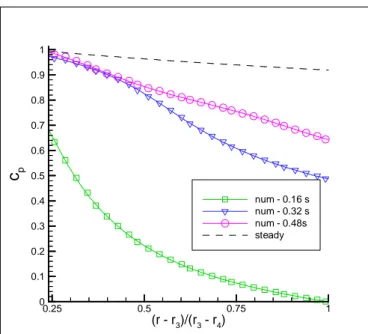
At last, the results of the model are used to predict qualitatively the performance of the diffuser during the start-up. To do so, the following non dimensional pressure coefficient is introduced and plotted Fig. 12:
−
−
=
2 21
2
1
)
(
)
(
r
R
c
p
r
p
r
c
inlet inlet inlet pρ
(7)Where
p
(
r
)
−
p
inlet is the static pressure rise predictedat each radius by the model and
−
2 21
2
1
r
R
c
inlet inletρ
the static pressure rise in the case of a steady , 1D, non viscous flow in the diffuser. It can be noticed that,
c
p(
R
outlet)
is corresponding to a recovery pressure factor. To be able to evaluate the transient effects on the pressure evolution, the evolution ofc
p in the case of a steady flow is also plotted (in this case, the inlet flow angle was considered to beα
=
14
°
. This angle is corresponding to the inlet flow angle at three time steps (t = 0.16, 0.32 and 0.48 s) plotted.0.25 0.5 0.75 1 (r - r3)/(r3- r4) 0 0.1 0.2 0.3 0.4 0.5 0.6 0.7 0.8 0.9 1
c
p num - 0.16 s num - 0.32 s num - 0.48s steadyFigure 12: Evolution of the pressure coefficient with radius at three time steps – numerical results.
At the beginning of the start-up (t=0.12s, Fig 12), the performance of the diffuser is very badly affected by the transient and the pressure at the outlet of the diffuser is equal to the one at inlet. At t = 0.32 s and t = 0.48 s, the evolution of the pressure coefficient is less affected by the transient effects and the pressure recovery is better but still less good than it would have been in steady operation. It can be noticed that the evolution of the pressure coefficients at t = 0.32 s and t = 0.48 s are very similar as long as r is lower than 0.315m. On the contrary, if greater radii are considered, the pressure coefficient is decreasing faster with radius at t = 0.32 s compared with the evolution at t = 0.48 s. These evolutions could be very well correlated with the evolutions of the flow angle (Fig. 13). The flow angles at diffuser inlet are similar for the three time steps considered. But, at t=0.16 s, the flow angle is increasing very rapidly (because of a quick decrease of the tangential velocity component – Fig. 11) and simultaneously the pressure
coefficient is decreasing also rapidly. The flow angles at t = 0.32 s and t = 0.48 s have very similar and moderate evolutions for radii lower than r = 0.315 m (as it was the case for the pressure coefficient), whereas for radii upper than 0.315 m, the flow angle is increasing more rapidly at t=0.32 s than at t=0.48s and simultaneously, the pressure coefficient is decreasing also rapidly. 0.3 0.4 0.5 0.6 0.7 0.8 0.9 1 (r - r3) / (r3- r4) 0 10 20 30 40 50 60 70 80 90 α ( ) num - t = 0.16 s num - t = 0.32 s num - t = 0.48 s o
Figure 13 ; Evolution of the flow angle with radius at three time steps – numerical results.
These evolutions of the pressure coefficient can be explained by the radial momentum equation (6) which can be rewritten as follows : r f r r u
c
c
b
c
t
c
r
c
r
c
r
P
.
)
(
1
2 2−
∂
∂
−
+
+
=
∂
∂
ρ
(8)The pressure increase in a diffuser is directly linked with the decrease of the kinetic energy. This is the balance between the left hand side and the two first terms of the right hand side of equation (8). But when the flow angle is increasing, this is because the tangential velocity is decreasing. Consequently, the first term on the right hand side of equation (8) is low whereas the third term of the right hand side (the unsteady term) which represents the inertial effect is depending only on the radial velocity component and is not affected by a tangential velocity component severe decrease. It could then affect badly the pressure evolution in the diffuser and its performance.
CONCLUSION
Some new experiments associating high speed stereoscopic PIV as well as pressure measurements in a vaneless diffuser in transient operation were performed. The analysis of the results have showed that the first period of the start-up is characterised near the diffuser inlet by tangential velocities of the order of the pump peripheral velocity and near the diffuser outlet by tangential velocity equal to zero. The comparison of the
experimental results with the ones obtained with a 1D numerical model have shown that the radial velocity is underestimated by the model probably because of the boundary layer growth is not taken into account by the model. Concerning the tangential velocities, the convection of the higher velocity at the inlet of the diffuser by the radial velocity component is qualitatively well predicted but quantitatively underestimated probably because of the underestimation of the radial velocity. The evolution of a pressure coefficient in the diffuser shows a negative effect of the transient on the diffuser performance, especially in the regions where the tangential velocity component is decreasing rapidly.
ACKNOWLEDGMENTS
The authors which to thank the CISIT program form Region Nord Pas de Calais for their support to this program research.
REFERENCES
[1] Tsukamoto H., Ohashi H., (1982) Transient Characteristics
of a Centrifugal Pump During Starting Period, Journal of
Fluids Engineering. Transactions of ASME, vol. 104, pp. 6 – 14
[2] Saito S. (1982) The Transient Characteristics of a Pump
During Start Up, Bulletin of JSME, vol. 25, n° 201, paper
n°201-10, pp. 372 – 379
[3] Ghelici N., (1993) Etude du régime transitoire de
démarrage rapide d’une pompe centrifuge, PhD Thesis.
Ecole Nationale Supérieure d’Arts et Métiers.
[4] Bolpaire S. (2000) Etude des écoulements instationnaires
dans une pompe en régime de démarrage ou en régime établi. PhD Thesis. Ecole Nationale Supérieure des Arts et
Métiers.
[5] Lefebvre P. J., Barker W. P. (1995) Centrifugal Pump
Performance During Transient Operation, Journal of
Fluids Engineering, vol. 117, pp 123 – 128
[6] Tsukamoto H, Matsunaga S, Yoneda H (1986), Transient
characteristics of a centrifugal pump during stopping period. ASME Journal of Fluid Engineering, 108(4):
392-399.
[7] Picavet A, (1996) Etude des phénomènes hydrauliques
transitoires lors du démarrage rapide d’une pompe centrifuge, PhD Thesis. Ecole Nationale Supérieure d’Arts
et Métiers.
[8] Tsukamoto H., Yoneda H., Sagara K., (1995) The response
of a centrifugal pump to fluctuating rotational speed.
ASME Journal of Fluids Engineering, vol. 117, pp 479 – 484.
[9] Tanaka T., H. Tsukamoto, (1999) Transient behaviour of a
cavitating centrifugal pump at rapid change in operating conditions—Part 1: Transient phenomena at
opening/closure of discharge valve. ASME Journal of
Fluids Engineering, 121, 841-849.
[10] Tanaka T., H. Tsukamoto, (1999) Transient behaviour of a
cavitating centrifugal pump at rapid change in operating
conditions—Part 2: Transient phenomena at pump Start-up/Shutdown. ASME Journal of Fluids Engineering, 121,
850-856,
[11] Tanaka T., H. Tsukamoto (1999), Transient behaviour of a
cavitating centrifugal pump at rapid change in operating conditions—Part 3: Classifications of transient phenomena.
ASME Journal of Fluids Engineering, 121, 857-865, [12] Duplaa Sébastien; Coutier Delgosha Olivier;
Dazin Antoine; Roussette Olivier; Bois Gérard;
Caignaert Guy (2010), Experimental Study of a Cavitating
Centrifugal Pump During Fast Startups. ASME Journal of
Fluids Engineering, 132 (2)
[13] Dazin A., Caignaert G., Bois G. (2007), Transient Behavior
of Turbomachineries: Applications to Radial Flow Pump Startups.ASME Journal of Fluids Engineering, 129 (11).
[14] Wuibaut G., Dupont P., Bois, G., Caignaert G., Stanislas M. (2001), Analysis of flow velocities within the impeller and
the vaneless diffuser of a radial flow pump. ImechE Journal
of Power and Energy, part A, vol. 215, pp. 801-808.
[15] Wuibaut G., Dupont P., Bois G., Caignaert G., Stanislas M. (2001), Application de la vélocimétrie par images de
particules à la mesure simultanée de champs d’écoulements dans la roue et le diffuseur d’une pompe centrifuge. La
Houille Blanche, revue internationale de l’eau, N° 2/2001, pp. 75-80.
[16] Wuibaut G., Bois G., Dupont P., Caignaert G., Stanislas M. (2002), PIV measurements in the impeller and the
vaneless diffuser of a radial flow pump in design and off-design operating conditions. ASME Journal of Fluids
Engineering, vol. 124, no. 3, pp. 791–797.
[17] Cavazzini G., Pavesi G., Ardizzon G., Dupont P., Coudert S., Caignaert G., Bois G. (2009), Analysis of the Rotor-tator
Interaction in a Radial Flow Pump. La Houille Blanche,
Revue Internationale de l’eau, n. 5/2009, pp. 141-151. [18] Dazin A. , Coutier-Delgosha O; Dupont P.; Coudert S.;
Caignaert G.; Bois G. (2008), Rotating Instability in the Vaneless Diffuser of a Radial Flow Pump. Journal of Thermal Science. Dec 2008, 17(4), 368-374.
[19] A. Dazin, G. Cavazzini, G. Pavesi, P. Dupont, S. Coudert, G. Ardizzon, G. Caignaert and G. Bois (2011) High Speed
Stereoscopic PIV Study of Rotating Instabilities in a Radial Vaneless Diffuser. Experiments in Fluids, DOI:
10.1007/s00348-010-1030-x
[20] Cheng Y.S., Bechtold W.E., Yu C.C, Huang I.F., (1995),
Incense smoke: Characterization and dynamics in Indoor Environments, Aerosol Sci. Technol. 23: 271-281.
[21] Soloff, S.M., Adrian, R.J., and Liu, Z.C., (1997) Distortion
compensation for generalized stereoscopic particle image velocimetry. Meas. Sci. Technol, 8, pp. 1441-1454.
[22] Foucaut J.M., Milliat B., Perenne N., Stanislas M., (2004), Characterisation of different PIV algorithms using the EUROPIV synthetic image generator and real images from a turbulent boundary layer. Proceeding of the EUROPIV 2 workshop on Particle Image Velocimetry. Springer, Berlin Heidelberg New York, pp 163-186.