HAL Id: hal-02559281
https://hal.archives-ouvertes.fr/hal-02559281
Submitted on 30 Apr 2020
HAL is a multi-disciplinary open access
archive for the deposit and dissemination of
sci-entific research documents, whether they are
pub-lished or not. The documents may come from
teaching and research institutions in France or
abroad, or from public or private research centers.
L’archive ouverte pluridisciplinaire HAL, est
destinée au dépôt et à la diffusion de documents
scientifiques de niveau recherche, publiés ou non,
émanant des établissements d’enseignement et de
recherche français ou étrangers, des laboratoires
publics ou privés.
SEGMENTATION OF RETINAL ARTERIAL
BIFURCATIONS IN 2D ADAPTIVE OPTICS
OPHTHALMOSCOPY IMAGES
Iyed Trimeche, Florence Rossant, Isabelle Bloch, Michel Pâques
To cite this version:
Iyed Trimeche, Florence Rossant, Isabelle Bloch, Michel Pâques. SEGMENTATION OF RETINAL
ARTERIAL BIFURCATIONS IN 2D ADAPTIVE OPTICS OPHTHALMOSCOPY IMAGES.
Inter-national Conference on Image Processing, Sep 2019, TAIPEI, Taiwan. �10.1109/ICIP.2019.8803076�.
�hal-02559281�
SEGMENTATION OF RETINAL ARTERIAL BIFURCATIONS IN 2D ADAPTIVE OPTICS
OPHTHALMOSCOPY IMAGES
Iyed Trimeche
1,2,3, Florence Rossant
1, Isabelle Bloch
2, Michel Paques
31. Institut Sup´erieur d’Electronique de Paris (ISEP), Paris, France
2. LTCI, T´el´ecom ParisTech, Universit´e Paris-Saclay, Paris, France
3. Clinical Investigation Center 1423, Quinze-Vingts Hospital, Paris, France
iyed.trimeche@isep.fr
ABSTRACT
The study of vascular morphometry requires segmenting vessels with high precision. Of particular clinical interest is the morpho-metric analysis of arterial bifurcations in Adaptive Optics Ophthal-moscopy (AOO) images of eye fundus. In this paper, we extend our previous approach for segmenting retinal vessel branches to the segmentation of bifurcations. This enables us to recover the mi-crovascular tree and extract biomarkers that charactarize the blood flow. Segmentation results are shown to be within the range of intra-and inter-user variability, allowing a preliminary study on biomark-ers derived from vessel diameter estimates at arterial bifurcations.
Index Terms— Active contours, segmentation, retinal arterial bifurcations, adaptive optics ophthalmoscopy images.
1. INTRODUCTION
This study aims to determine the effect of CADASIL syndrome on vessel morphometry, by segmenting retinal vessels precisely in Adaptive Optics Ophthalmoscopy (AOO) and then derive some biomarkers. This rare pathology is an inherited condition that causes stroke and other impairments affecting blood flow in small blood vessels, particularly vessels within the brain [1]. Retinal vessels are related to cerebral vessels, sharing many structural, functional, and pathological features. Therefore, retinal vessels may be considered in many ways as substitutes for the cerebral vessels. Moreover, they are more easily observable thanks to their planar arrangement and to dedicated high resolution imaging systems, such as AOO (Fig. 1). For all these reasons, we can assume that the analysis of retinal vessel alterations observable in 2D AOO images will enable us to define relevant biomarkers for CADASIL syndrome.
In addition to the general considerations of contrast, resolution, noise and acquisition dependent artifacts, retinal vascular networks are complex tree-like structures with successive branchings. To analyze these structures, the relationships between the lumens (i.e. diameters) of bifurcating blood vessels are shown to arise from some simple principles of optimality, as already suggested by D’Arcy Thompson [2]. The best known of these is Murray’s law [3]. This law led to the definition of many biomarkers that describe the rela-tionship between parent vessel and child branches in a bifurcation. Measuring diameter dependent biomarkers on patients has shown deviations from Murray’s optimality, related with some pathologies such as stroke [4], diabetes [5] and high blood pressure [6]. These
This research has been partially funded by a grant from the French Agence Nationale de la Recherche ANR-16-RHUS-0004 (RHU TRT cSVD).
deviations can be related to blood circulation disorders and reflect the progress of some pathologies.
The estimation of retinal artery lumen at a bifurcation requires an accurate segmentation of the vascular tree, which is a very diffi-cult but also valuable task especially for studying vessel morphome-try and for diagnosis assistance [7]. In fact, most clinical studies rely on standard eye fundus images (the interior wall of the eye) [4, 6]. Limits of the proposed protocols come from the poor resolution of the images (about 10 to 20 µm/pixel) and the methods used to esti-mate the diameters. In [5], such estimations are based on manually defined points, so with limited accuracy and reproducibility. AOO offers a much higher image resolution (about 1 to 2 µm/pixel), and potentially more accurate biomarker estimates, but, to the best of our knowledge, there does not exist yet a fully automatic and reliable segmentation algorithm to this end.
This paper presents a semi-automatic method for precise seg-mentation of arterial bifurcations in 2D AOO images, which ex-tends our previous work on segmentation of individual arterial branches [8]. The algorithm segments the branches according to the method proposed in [8], then the segmentation is refined at bifurcations following our new approach. Diameter estimation at bifurcations is then performed, as well as a preliminary study of biomarker extraction on healthy and pathological cases. Finally, we evaluate quantitatively diameters and biomarkers measured from our segmentation.
Fig. 1: Segmentation of an AOO image of a retinal artery [8].
2. STATE OF THE ART
Conventional fundus photographs were generally used to estimate biomarkers at arterial bifurcation or venous confluences [5, 6]. AOO allows for a better resolution and hence a potentially more accurate estimate of diameters and biomarkers. Arichika et al. [9] segmented AOO images with a semi-automatic method: spline interpolation is applied to determine the limits of the vessel lumen from con-trol points placed manually, and then estimate the diameters. This approach is operator-dependent and lacks reproducibility; it is not tractable when processing large databases. A fully automatic method for segmenting artery walls was developed by Lerme et al. [8], who
proposed exploiting prior information on the geometry of the ves-sels and their gray levels in AOO images. This method models the arterial wall as four curves approximately parallel to a common ref-erence line placed on the central reflection (Fig. 1). These curves are initialized automatically through a tracking procedure and this initial segmentation is refined using an active contour model embed-ding a parallelism constraint [10]. This algorithm, called AOV, was meant to delineate the wall of any artery branch referenced by its central reflection, but does not provide an accurate segmentation at bifurcations. Contours cross at the bifurcation but do not follow the lumen borders (see Fig. 2a). Moreover, the fully automatic local-ization of central reflections (and so of the vessel branches) is not reliable enough.
Hence, in this article, we propose a new approach to segment accurately the bifurcations. It is based on three steps: (1) a man-ual step where the user defines the three vessel branches involved in the bifurcation by placing points on the central reflections; (2) the automatic segmentation of the branches by AOV algorithm; (3) the segmentation of the bifurcation, described in Section 3, which is the key contribution of this paper. This way, the tedious manual seg-mentation task is avoided, as the user’s action is limited to an easy initialization step, and the bifurcation segmentation itself is fully au-tomatic. Finally, the diameters are estimated.
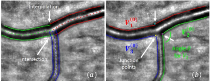
3. SEGMENTATION OF RETINAL BIFURCATIONS In this section, we present the proposed method for bifurcation segmentation. Starting from a manual initialization, i.e a set of points manually placed on the central reflection of the three vessel branches, we apply AOV [8] to segment them accurately. Fig. 2a shows the three pairs of curves that delineate the lumen of the vessel branches (the outer borders are not used in this study).
Fig. 2: Initialization of the active contour model. (a) Initial segmen-tation of vessel branches obtained with AOV semi-automatic mode. (b) Curves Vi(0)obtained after rearrangement of the 6 curves delin-eating the 3 branches involved in the bifurcation.
While this result is generally accurate along the vessel branches, this may not always be the case at the bifurcations. In this study, where diameters have to be measured closed to the bifurcations to derive relevant biomarkers, a precise segmentation is needed even at bifurcations. Therefore we propose to improve the previous re-sult in the following way. We detect the intersection points between two contours (see the crossing contours in Fig. 2a) and we eliminate the rest of the segmentation lines after their crossing. If there is no crossing of segmentation lines, a linear interpolation is applied to re-connect segmentation contours. The resulting curves are rearranged to obtain three segmentation lines, denoted by Vi(0), as shown in Fig. 2b. The locations of the former intersection or re-connection points are referred to as junction points and point out regions where
the segmentation has to be refined. This new configuration is consid-ered the initialization of an active contour model whose purpose is to ensure that the contours converge precisely to the inner wall of the vessels at the bifurcation without moving out of that region, where the initial segmentation was precise. We propose the following en-ergy functional to be minimized by this deformable model:
E(Vi) =R01− | ∇I(Vi(s)) | +α(s) | Vi0(s) |2+ϕ(s) | Vi(s) − Vi(0)(s) | 2ds (1)
where Viis one of the three contours, parametrized by s, and Vi(0)is the corresponding initial contour. In Eq. 1, the first term attracts Vi towards the strong gradients of the image, denoted by I. The second term is a first regularization for smoothing the curve at the bifurca-tions, and the last term is a second regularization which insures that the curve Vi remains close to the initialization Vi(0). The weights α(s) and ϕ(s) are defined according to two criteria, the angle of the re-connected curves at the junction point and the distance to this point. The aim is to impose a strong regularization when moving away from the junction point, to keep the initial position, and to re-lax the regularization around the junction point, so that the curve can accurately move towards the inner border of the lumen at the bifur-cation. This imposes ϕ(s) to be high for points far from the junction point and low around it. Moreover, we also take into account the angles of the reconnected curves at the junction point (Fig. 2b): we need a strong regularization for flat angles, so high values for α(s), and weak values for acute angles, to avoid shortcuts. Thus, to cal-culate the weight profiles, we rely on a function f(s0,δ)
p (s) of the curvilinear abscissa s, parametrized by the position s0 of the junc-tion point and a margin δ around it (Fig. 3):
f(s0,δ)
p (s) = max(1+exp(−(s−s1
0−δ)),
1
1+exp(−(s0−s−δ))) (2)
The margin δ is calculated from a rough estimate of the mean di-ameters db1and db2 of the two branches involved in the processed contour Vi(s):
δ = min(db1, db2) (3)
Fig. 3: Function f(s0,δ)
p (s) parameterized by the curvilinear abscissa s0of the junction point and the margin δ around it.
Then, the value of ϕ is simply given by: ϕ(s) = ϕ0f(s0,δ)
p (s) (4)
with ϕ0= 10. Thus, the proximity constraint with respect to the ini-tial curve is totally relaxed at the bifurcation, over a distance com-parable to the smallest diameter of the two branches involved. It is weighted by ϕ0otherwise.
The second weight α(s) follows a similar profile (Eq. 2, Fig. 3) but it evolves between a maximum value αhigh, set experimentally, and a minimal value αmincalculated from the angle θ formed by the two initial curves at the junction point (Fig. 2b) :
where γ = 0.1, αlow = 10, αhigh = 75 and θmed = 115◦. Thus, the value αminranges between αlow and αhigh, with high values for flat angles and low values for acute angles (Fig. 4a). Then, the weight α(s) is again defined by the profile function f(s0,δ)
p (s) in order to modulate the regularization constraints according to the dis-tance to the bifurcation:
α(s) = αmin+ (αhigh− αmin)f(s0,δ)
p (s) (6) Fig. 4b shows the profile we finally obtain for α(s) for the three curves delineating the bifurcation in our example of Fig. 2b. The regularization is high for points far from the junction points, to get smooth curves, and lower around the bifurcation. The more acute the angle, the more relaxed the constraint: for example, αmin' 13 for V3(blue curve) for which θ = 84◦while αmin' αhighfor V1 (red curve) where θ = 166◦.
Fig. 4: Calculation of α(s). (a) Determination of αminas a function of the angle at the bifurcation. (b) Profiles α(s) for the three contours (s in pixels), parametrized by the abscissa s0of the junction point, the margin δ and the calculated minimum value αmin.
The energy functional E(Vi) (Eq. 1) is classically minimized by solving numerically the associated Euler-Lagrange equation [11]. The active contour model is applied on the three curves Vi indepen-dently. This last segmentation step leads to a precise and regular segmentation of the bifurcation (Fig. 5). Moreover, it respects the initial segmentation of the branches. The functions α and ϕ have a suitable profile while being differentiable. There are five parameters to set: ϕ0, αlow, αhigh, θmedand the factor γ setting the slope of αmin(θ) (Eq. 5, Fig. 4a). We tuned them empirically on a subset of five images representative of the angles and diameters we have in our dataset, just by observing the behavior of the model. We also verified that the final values are not too sensitive, by checking that the final segmentation does not vary significantly if we shift slightly one parameter. Once these parameters are definitively fixed, the pro-posed method adapts itself to the geometry of the vessel branches, without any tuning. User’s action is limited to the initialization step of the central reflections, an easy step which does not need to be precise. The next steps are fully automatic, which ensures a good reproducibility of segmentation results.
4. EXPERIMENTS
4.1. Adaptive optics images and acquisition protocol
To carry out this study, we have built an AO database of control, di-abetic and CADASIL subjects, in order to make a statistical study of bifurcation morphometry in each pathology. The rtx1 AOO camera from Imagine Eyes enables to visualize microscopic retinal struc-tures with high resolution (pixel size equal to 0.8 µm, corresponding to a physical resolution of 1.6 µm/pixel), non-invasively and without using contrast agents. Several images of the eye fundus were ac-quired, tracking one main artery emerging from the optic disk up to
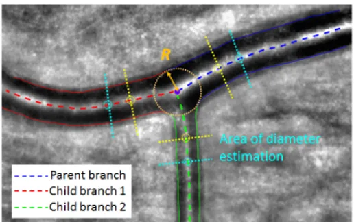
Fig. 5: Final segmentation and areas of diameter estimation.
the sixth bifurcation. Diameters of the acquired branches range from 90 µm to 20 µm for the smallest arterioles. Images were acquired from 23 control subjects, 28 patients with non-proliferative diabetes (NDR) and 25 patients with CADASIL syndrome. Each subject first underwent an ophthalmic examination, and visual control was done to ensure that the images were not blurred.
4.2. Biomarker measurements
Arterial bifurcation morphometry can be evaluated by measuring biomarkers derived from Murray’s law [3]. The most known is the junction exponent x defined by:
dx0 = d x 1+ d
x
2 (7)
where d0is the parent diameter while d1and d2are the child diam-eters. Murray stated that x = 3 for an ideal bifurcation. Clinical studies have shown a deviation of the junction exponent from this optimal value in peripheral arterial diseases [6], incident heart dis-ease, stroke [4] and diabetes [5]. Nevertheless, solving Eq. 7 may lead to negative values of x, which has no physiological interpreta-tion. This may happen in particular for pathological subjects [4]. For this reason, we have selected another biomarker, that is derived from the branching coefficient, defined by:
βmeasured=d 2 1+ d22 d2 0 = 1 + λ 2 (1 + λx)2/x (8) where λ = d2/d1 (d2 < d1) measures the asymmetry of child branches. Considering an ideal bifurcation with an asymmetry coef-ficient λ, the optimal branching coefcoef-ficient βoptimalis given by the right hand side of Eq. 8 with x = 3. Therefore, we calculate the deviation βdevto the optimal branching coefficient:
βdev= βoptimal− βmeasured (9) This biomarker is always calculable and provides information on the deviation to Murray’s law optimum. In practice, we estimate the branch diameters in regions derived from the largest circle inscribed in the bifurcation (i.e. tangent to the segmentation), similarly to [12]. Let us denote by R the radius of this circle. The measurement re-gion starts at a distance equal to one radius R from the intersection point between the circle and the central reflection, up to 2R (see Fig. 5). We calculate the median of the diameters measured in this region (more robust to outliers than the mean value). Fig. 6 shows the biomarkers we obtained on our database.
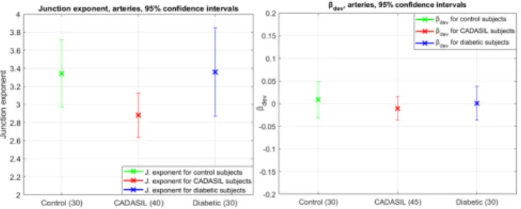
For the results for βdev, we note a deviation in the positive di-rection of Murray’s law which is consistent with [5] for the com-parison between healthy and diabetic subjects. Yet, there is a trend toward a negative deviation for CADASIL subjects, which may in-dicate downstream increase of flow resistivity.
Fig. 6: Results for control subjects, diabetics and CADASIL at a 95% confidence interval. Left: junction exponent x (cases with x > 0 only). Right: deviation βdevto the optimal branching coefficient.
4.3. Quantitative evaluation
Ten images (not trained) were selected from the database for the quantitative evaluation. This selection was done by the medical ex-perts to ensure representativeness in terms of image quality and mor-phology variability encountered in clinical routine. Three physicians (P hysj) segmented manually the set of images. Five images were processed twice by each physician to study the intra-expert variabil-ity. Let us denote by Vi(Seg) and V
(Ref )
i two distinct segmenta-tions of the contour Vi, where Vi(Ref )is chosen as a reference and Vi(Seg)as a segmentation to evaluate. The segmentation accuracy is given by the mean squared error (MSE) between the curves Vi(Ref ) and Vi(Seg), calculated on a circular region centered on the bifur-cation and of radius 4R. Then, we estimated the median diameters d as described above, for each branch, in the segmentation and in the reference and, finally, the derived biomarkers. We denote by δd0,1,2, δβdev and δx the measured differences (averaged for the three branches for the diameters). The results are then averaged over the test cases to obtain mean and standard deviation values. Table 1 shows the intra-expert variability measured from the five segmen-tations realized twice by each expert. The physician P hys3, who obtained the most stable results on the biomarkers, was chosen as reference for the inter-experts and software/expert variability study. Table 2 summarizes the results obtained on the 10 images. Examples are shown in Fig. 7.
MSE δd0,1,2 δβdev δx
P hys1 2.43 ± 0.90 +0.84 ± 2.22 0.00 ± 0.09 −0.10 ± 0.49
P hys2 2.80 ± 0.99 −0.62 ± 3.98 0.00 ± 0.11 +0.41 ± 1.24
P hys3 2.04 ± 0.96 −1.18 ± 2.09 +0.01 ± 0.02 +0.07 ± 0.11
Table 1: Intra-expert variability (MSE and diameters expressed in pixels).
Seg/Ref MSE δd0,1,2 δβdev δx
P hys1/P hys3 2.65 ± 1.48 +0.06 ± 4.51 −0.04 ± 0.07 −0.44 ± 1.20
P hys2/P hys3 3.25 ± 1.84 +0.52 ± 6.15 0.00 ± 0.18 −0.40 ± 2.24
Sof tware/P hys3 3.22 ± 1.21 +2.78 ± 2.95 +0.02 ± 0.06 +0.11 ± 0.38
Table 2: Inter-expert variability and software/expert variability. Values are expressed in pixels for MSE and diameters.
The proposed method leads to MSE values within the same range as the inter-experts variability and slightly higher than the intra-expert variability. This demonstrates the accuracy of the pro-posed segmentation method. Considering the diameters, estimation errors are consistent with the measured M SE but we note a positive bias that reveals a small over-segmentation, however with a smaller standard deviation than for the inter-experts evaluation. Neverthe-less, our automatic method reaches the best accuracy regarding the
biomarkers, both in terms of mean error and standard deviation, similar to the intra-expert accuracy and better than the inter-experts accuracy. However these errors are quite significant regarding the targeted application (Fig. 6), especially for βdev. This biomarker is always calculable but maybe more sensitive to segmentation imprecision than the junction exponent. This needs to be further investigated through a statistical analysis of significance. Examples are illustrated in Fig. 7. In (b), the blur on the child branch 2 (red arrow) leads to an uncertainty on the border localization, which results in significant differences between the manual and automatic estimates of d2 and of the biomarkers. This study shows the diffi-culty of estimating biomarkers characterizing arterial bifurcations, despite the high resolution of AOO. The main limitation is due to the blur in the images, when the bifurcation is not exactly in the focal plane, which leads to uncertainty in the delineation of the lumen, even for experts.
Fig. 7: Examples of segmentations and biomarker estimations. The manual segmentations are represented in yellow dashed curves.
5. CONCLUSION
We have proposed a method to segment arterial bifurcations in AOO, based on our previous approach for segmenting artery branches [8]. A new active contour model has been designed, to refine the seg-mentation at bifurcations. It is based on adaptive weighting of two regularization terms to cope with the specific geometry of every bi-furcation and keep the initial segmentation where it is reliable. The quantitative evaluation has demonstrated a good accuracy of the pro-posed approach, with MSE values within the range of inter-experts variability. We have also shown promising preliminary results on biomarkers extracted from these segmentations to characterize pathologies. Future work aims at automatically evaluating the relia-bility of the diameter estimates, in order to discard biased biomarker values and better characterize CADASIL pathology. Moreover, it is now possible to consider the vascular tree as a whole, so to analyze blood circulation more globally.
Acknowledgments. The authors would like to thank Dr. V. Krivosic and Dr. C. Lavia of the ophthalmology department of Lariboisi`ere hospital for providing AOO images, and the ophthalmologists of Quinze-Vingts Hospital for providing AOO images and for perform-ing manual segmentations.
6. REFERENCES
[1] H. Chabriat, A. Joutel, M. Dichgans, E. Tournier-Lasserve, and M.-G. Bousser, “Cadasil,” The Lancet Neurology, vol. 8, no. 7, pp. 643–653, 2009.
[2] D’A. W. Thompson, On growth and form., Cambridge Uni-versity Press, 1942.
[3] C. D. Murray, “The physiological principle of minimum work: I. the vascular system and the cost of blood volume,” Proceed-ings of the National Academy of Sciences, vol. 12, no. 3, pp. 207–214, 1926.
[4] N. W. Witt, N. Chapman, S. A. McG. Thom, A. V. Stanton, K. H. Parker, and A. D. Hughes, “A novel measure to char-acterise optimality of diameter relationships at retinal vascular bifurcations,” Artery Research, vol. 4, no. 3, pp. 75–80, 2010. [5] T. Luo, T. J. Gast, T. J. Vermeer, and S. A. Burns, “Retinal vascular branching in healthy and diabetic subjects,” Inves-tigative Ophthalmology & Visual Science, vol. 58, no. 5, pp. 2685–2694, 2017.
[6] N. Chapman, N. Witt, X. Gao, A.A. Bharath, A.V. Stanton, S.A. Thom, and A.D. Hughes, “Computer algorithms for the automated measurement of retinal arteriolar diameters,” British Journal of Ophthalmology, vol. 85, no. 1, pp. 74–79, 2001.
[7] D. Lesage, E. D. Angelini, G. Funka-Lea, and I. Bloch, “A review of 3D vessel lumen segmentation techniques: Models, features and extraction schemes,” Medical Image Analysis, vol. 13, pp. 819–845, 2009.
[8] N. Lerm´e, F. Rossant, I. Bloch, M. Paques, E. Koch, and J. Benesty, “A fully automatic method for segmenting retinal artery walls in adaptive optics images,” Pattern Recognition Letters, vol. 72, pp. 72–81, 2016.
[9] S. Arichika, A. Uji, S. Ooto, Y. Muraoka, and N. Yoshimura, “Comparison of retinal vessel measurements using adaptive optics scanning laser ophthalmoscopy and optical coherence tomography,” Japanese Journal of Ophthalmology, vol. 60, no. 3, pp. 166–171, 2016.
[10] F. Rossant, I. Bloch, I. Ghorbel, and M. Paques, “Parallel dou-ble snakes. Application to the segmentation of retinal layers in 2D-OCT for pathological subjects,” Pattern Recognition, vol. 48, pp. 3857–3870, 2015.
[11] M. Kass, A. Witkin, and D. Terzopoulos, “Snakes: Active contour models,” International Journal of Computer Vision, vol. 1, no. 4, pp. 321–331, 1988.
[12] S. Ramcharitar, Y. Onuma, J.-P. Aben, C. Consten, B. Weijers, M.-A. Morel, and P. W Serruys, “A novel dedicated quanti-tative coronary analysis methodology for bifurcation lesions.,” EuroIntervention: Journal of EuroPCR in collaboration with the Working Group on Interventional Cardiology of the Euro-pean Society of Cardiology, vol. 3, no. 5, pp. 553–557, 2008.
![Fig. 1: Segmentation of an AOO image of a retinal artery [8].](https://thumb-eu.123doks.com/thumbv2/123doknet/11422892.288982/2.918.528.786.767.846/fig-segmentation-aoo-image-retinal-artery.webp)