Reedbed monitoring using classification trees and SPOT-5 seasonal time series

HAL Id: hal-00692542

https://hal.archives-ouvertes.fr/hal-00692542

Submitted on 30 Apr 2012

HAL is a multi-disciplinary open access

archive for the deposit and dissemination of

sci-entific research documents, whether they are

pub-lished or not. The documents may come from

teaching and research institutions in France or

abroad, or from public or private research centers.

L’archive ouverte pluridisciplinaire HAL, est

destinée au dépôt et à la diffusion de documents

scientifiques de niveau recherche, publiés ou non,

émanant des établissements d’enseignement et de

recherche français ou étrangers, des laboratoires

publics ou privés.

Reedbed monitoring using classification trees and

SPOT-5 seasonal time series

Aurélie Davranche, Brigitte Poulin, Gaëtan Lefebvre

To cite this version:

Aurélie Davranche, Brigitte Poulin, Gaëtan Lefebvre. Reedbed monitoring using classification trees

and SPOT-5 seasonal time series. International Symposium on Advanced Methods of Monitoring

Reed Habitats in Europe, Nov 2010, Illmitz, Austria. pp.15-29. �hal-00692542�

Reedbed monitoring using classification trees and

SPOT-5 seasonal time series

Aurélie Davranche, Institut für Geographie, Friedrich-Alexander Universität Erlangen-Nürnberg, Erlangen, Germany; Brigitte Poulin, Tour du Valat Research Center, Arles, France Gaëtan Lefebvre,

Tour du Valat Research Center, Arles, France

Keywords

:

Abstract

The Camargue, the Rhône river delta in south of France, has lost 40,000 ha of natural areas, including 33,000 ha of wetlands over the last 60 years, following the extension of agriculture, salt exploitation and industry. Reed development and density in Camargue marshes is influenced by physical factors such as salinity, water depth, and water level fluctuations, which have an effect on reflectance spectra. Classification trees applied to time series of SPOT-5 images appear as a powerful and reliable tool for monitoring wetland vegetation experiencing different hydrological regimes. The resulting tree provided a cross-validation accuracy of 98.7% and a mapping accuracy of 98.6% (2005) and 98.1% (2006). Misclassifications were partly explained by digitizing inaccuracies, and were not related to biophysical parameters of reedbeds. The resolution of SPOT-5 scenes provides an adequate scale for acquiring detailed field data within homogeneous stands, allowing to optimize the time spent for data collecting and to properly locate the sampled plots on the ground and on the scenes. Our results demonstrate that it is possible with a good field campaign to avoid repeated sampling for a long-term cost-efficient monitoring of reed marshes. The accuracy and reliability of our models provide a vision where the roles are reversed: the field campaigns become a complementary tool in wetland monitoring using satellite remote sensing.

1 Introduction

Efficient, accurate and robust tools for monitoring wetlands over large areas are urgently needed following their destruction and degradation, in spite of the many services and functions they provide to human kind (Özesmi & Bauer, 2002). Methods used for mapping their distribution should be simple to understand and easy to interpret in order to contribute to management advising. Satellite remote sensing presents many advantages for inventorying and monitoring all types of wetlands (Özesmi & Bauer, 2002). However, flooded areas pose unusual challenges for field campaigns, and class imbalance in remote sensing of wetlands is a well-known problem (Wright & Gallant, 2007). Spatial studies of these ecosystems require flexible and robust analytical methods to deal with non-linear relationships, high-order interactions, and missing data. Non-parametric classifiers such as rule-based methods are an alternative to traditional remote sensing techniques to enhance the accuracy of wetland classification (Sader et al., 1995; Özesmi, 2000; Baker et al., 2006). Because classification trees (CTs) easily accommodate data from all measurements scales, they are useful for distinguishing spectral similarities among wetlands with ancillary environmental data (Wright & Gallant, 2007). Seasonal time series of satellite multispectral data may provide, through the use of Classification Trees (CTs), reliable, replicable and understandable tools for wetland monitoring. The aim of this study is to evaluate the potential of CTs and multiseasonal SPOT-5 images to model the presence of common reed (Phragmite australis) stands in Camargue. The development of this space based model of reed beds distribution, described below, has been published in further details in Davranche et al. (2010).

2 Methods

2.1 Study site and habitat description

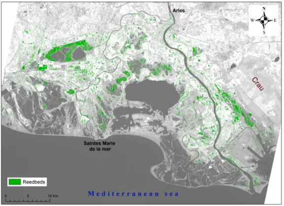
The study area is the Camargue or Rhône river delta covering 145,000 ha near the Mediterranean Sea in southern France. The Camargue consists mainly of agricultural land (mostly rice) mixed with natural or semi-natural brackish marshes either covered with submerged marcrophytes (Potamogeton, Myriophyllum, Ruppia, and Chara) or tall helophytes (mostly common reed Phragmites australis but also club rush Bolboschoenus maritimus, Schoenoplectus littoralis, S. lacustris and cattail Typha angustifolia, T. latifolia). The climate is Mediterranean with mild and windy winters and hot and dry summers. Mean annual rainfall over the last 30 years is 579±158 (SD) mm, being concentrated in spring and autumn, with large intra and inter-annual variations (Chauvelon, 2009). A large part of the marshes located in private estates, has been fragmented and intensively managed through freshwater inputs for socio-economic activities such as waterfowl hunting, reed harvesting, and cattle grazing. Therefore, vegetation development and density in Camargue marshes is influenced by physical factors such as salinity, water depth, and water level fluctuations, which have an effect on reflectance spectra (Silvestri et al., 2002). In the Camargue, common reed can form monospecific stands overlarge areas in shallow marshes or develop linearly along canals. Aerial stems emerge during spring and reach their maximum growth at the end of June. The inflorescences or panicles start developing in July and turn purplish-brown with a fluffy aspect at maturation in autumn. Seeds are wind-dispersed in early winter with the panicles becoming thinner and switching to a beige colour. Leaves remain green until October and turn yellow before drying and falling down in winter. The stems then dry but stand for a few years before breaking down. In order to provide sustainable conditions for reed harvesting in winter, reedbeds are flooded from March to June, dried in summer, flooded in autumn and drained in winter for mechanical harvest (December– March). Flooding can be extended through spring or summer if waterfowl hunting occurs. The total area of reedbeds in the Camargue has been estimated at about 8000 ha, of which 2000 ha is harvested every year (Mathevet & Sandoz, 1999).

2.2 Data

2.2.1 Land cover data

The training sample, collected in 2005, consisted of 46 plots of common reed spread throughout the Camargue. The independent validation sample of 2006 consisted of 21 sites. Water and vegetation measures were taken within 20×20m squares (i.e., four pixels of a SPOT-5 scene) of homogeneous vegetation placed within a larger homogeneous zone and located at least 70m from the border to reduce edge effects in spectral response. Each sampling plot was placed in a different hydrological unit to increase structural diversity and avoid autocorrelation. They were geolocated with a GPS (Holux GR-230XX). Water level, plant cover and composition were estimated along two diagonals crossing the entire plot. Common reed density was measured by counting the green and dry stems inside four quadrats of 50×50 cm per plot in June or July located at 7m from the center of the plot in each cardinal direction. Homogeneity throughout the plot was visually estimated and coded from 1 to 4. Vegetation cover was evaluated with four digital pictures taken vertically from the ground level upwards in the centre of the 50-cm quadrats and processed with CANEYE (Baret & Weiss, 2004). Water levels were measured at a permanent rule during vegetation sampling, as well as monthly or twice monthly at each hydrological unit sampled. Other land cover types were extracted from a vector layer created by the Réserve Nationale de Camargue from aerial photographs in 2001 provided by the Parc Naturel Régional de Camargue and additional digitalizing based on aerial photographs and ground or aerial (airplane and ultra-light aircrafts) surveys. In 2006, an updated land cover was available, providing details for agricultural crops.

2.2.2 Satellite remote sensing data

The Camargue can be covered with a single SPOT-5 scene (60×60 km). Two seasonal time series of SPOT-5 images (SPOT/ Programme ISIS. Copyright CNES) and field datasets were acquired at one year intervals for model building (2004–2005) and validation (2005–2006). Thanks to the Spot satellite programming service, scenes were acquired in late December, March, May, June, July and September (October in 2006) of both years. SPOT-5 has 10-m spatial resolution and four bands: B1 (green: 0.50 to 0.59 µm), B2 (red: 0.61 to 0.68 µm), B3 (near-infrared NIR: 0.79 to 0.89 µm) and B4

(shortwave-infrared SWIR: 1.58 to 1.75 µm). Spot scenes came with radiometric correction that is the pre-processing level called 1A (Spot image, 2008). Scenes were radiometrically corrected using the 6S atmospheric code (Davranche et al., 2009) and projected to Lambert conformal conic projection datum NTF (Nouvelle Triangulation Française). We extracted the mean reflectance value for each plot of reed and each polygon of other land covers from each band of each scene using the ‘Spatial Analyst’ of ArcGis version 9.2 (Environmental Systems Research Institute, Meudon, France). Using these data, we further calculated for each plot and polygon the most common multispectral indices (Table 1), and multitemporal indices corresponding to subtractions between each pair combination of dates. In the data file, these variables were labelled as follow OSAVI_12 for the Optimized Soil Adjusted Vegetation Index of December and B3_0603 for the difference between March and June in the reflectance value of band B3.

Tab. 1: Multispectral indices used in this study.

2.3 Statistical modelling and mapping

CT analysis based on dichotomous partitioning (Breiman et al., 1984) was performed with the Rpart (Recursive PARTitioning, Therneau & Atkinson 1997) package in the R software using a class coded “1” for the presence of reed or submerged macrophyte beds and a class coded “0” for absence (= other land cover types detailed in Table 1). For the pruning phase, we used 10 cross-validation subsets. The optimally pruned tree was defined with the cp (cost complexity parameter, Breiman et al, 1984) providing the smallest overall classification error rate among 10 iterative runs of the algorithm. To improve classification accuracies with our unbalanced samples, the optimal prior parameter that gives the highest classification accuracy was selected using the iterative method proposed by Breiman et al. (1984). The equations issued from the resulting tree was applied to SPOT-5 scenes of 2005 for estimating model accuracy and to 2006 scenes for estimating model robustness. For this procedure we used the raster calculator (Spatial Analyst) of ArcGIS to create binary maps, with 1 encoded for the presence of reed and 0 for the presence of other land covers. Using the zonal statistics tool (Spatial Analyst) of ArcGIS, we extracted values 1 and 0 for each class of the validation sampling. As described by Wright and Gallant (2007), overall accuracies and omission error rates were calculated using the sample error matrix, whereas the commission and overall error rates were estimated from the population error matrix given from known numbers of reedbeds and other land covers in the study area.

To test the relevance of the variables selected in the model, their mean value and 95% confidence intervals were calculated for each class of the training and the validation samples. The binary response (0/1) for misclassified and well-classified plots in both years was confronted to structural parameters of reed considered individually, using the likelihood ratio test (Sokal & Rohlf, 1995) for model significance. The following parameters were examined for common reed: height of green stems, density of green and dry stems, dry-to-green stem ratio, diameter of green and dry stems, plot homogeneity, and percent cover of vegetation. A year variable was included as a potential parameter

Index Formula Reference

SR - Simple Ratio B2/B3 Pearson & Miller, 1972 VI - Vegetation Index B3/B2 Lillesand & Kiefer, 1987 DVI - Differential Vegetation Index B3-B2 Richardson & Everitt, 1992 MSI - Moisture Stress Index B4/B3 Hunt & Rock, 1989

NDVI - Normalized Difference VI (B3-B2)/(B3+B2) Rouse et al., 1973 SAVI - Soil Adjusted VI 1.5*(B3-B2)/(B3+B2+0.5) Huete, 1988

OSAVI – Optimized SAVI (B3-B2)/(B3+B2+0.16) Rondeaux et. al., 1996 NDWI – ND Water Index (B3-B4)/(B3+B4) Gao, 1996

NDWIF – NDWI of Mc Feeters (B1-B3)/(B1+B3) Mc Feeters, 1996 MNDWI – Modified NDWI (B1-B4)/(B1+B4) Hanqiu, 2006 DVW – Difference between V and W NDVI - NDWI Gond et al, 2004

for misclassification.

3. Results

The resulting classification tree for common reed (Fig. 1) provided a cross-validation accuracy of 98.7% with the equation: B3_0603≥ 0.04897 and OSAVI_12<0.2467 and MNDWI_09<−0.3834.

Fig. 1: Optimal tree for the common reed classification. Presence of common reed = 1, presence of other land covers=0. The number of sites assigned to 0 (on the left) and 1 (on the right) is indicated below each end node.

The map of common reed resulted in an overall accuracy of 98.6% in 2005 and 98.1% in 2006 (Fig. 2, Table 2). Common reed sites were incorrectly classified at 16.7% in 2005 and 11.5% in 2006. Misclassifications involved mostly tamarisks on both years, as well as club rush and sunflower in 2006 (Table 3).

Tab 2: Error rates and accuracy for maps of reed and aquatic beds in 2005 and 2006.

Omission error (%)

Overall accuracy

(%)

Commission error (%) Overall error (%)

Reedbeds Other land

covers Reedbeds

Other land covers

2005 16.7 1.4 98.6 22.9 1.0 2.2 2006 11.5 1.9 98.1 29.7 0.6 2.4

Tab 3: Omission error rates (%) for reed in 2005 and 2006 relative to other land cover types.

2005 2006

Land cover types Total class other land cover: 1.4 %

Total class other land cover: 1.9 % Sea 6362 0.0 0.0 Submerged macrophytes 99 0.0 0.0 Common reed 30 Tamarisk 1264 18.8 16.1 Riparian forest 8822 8.8 1.4 Sawgrass 93 0.0 0.0 Rush 6236 0.5 2.1 Grassland 8631 0.7 0.6 Sand 5370 0.1 0.5 Saline marsh 98047 0.0 0.0 Salt pan 42248 1.5 0.9 Urban 6669 4.5 4.7 Club rush 9 0.0 30.0 Other forests 3017 1.0 0.7 Sunflower 1709 23.2 Wheat 1241 5.4 Orchard 2319 0.0 Rape 1359 0.0 Vines 1395 8.4 Market gardening 611 3.8 Fallow land 2468 0.2 Corn 2031 0.2 Ploughed crop 746 13.5 Meadow 498 0.0 Rice 13278 7.8 All crops 27655 3.1 6.3

Considering the omission error rates of both classes, the total area covered by common reed in the Camargue is estimated at 8842 ha in 2005 and 9128 ha in 2006.

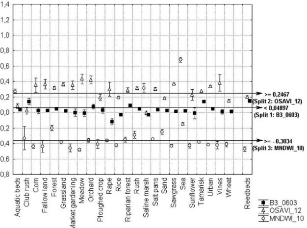
The variables selected in the models exhibited a similar range of variation in 2005 and 2006, suggesting that our approach might be robust for inter-annual applications. The 95% confidence interval of most variables for reed beds was far from the splitting values used for classification (Figs. 3-4).

Fig 3: Mean values and confidence intervals (95%) of each predictive variable in the reedbed model for each land cover class of the training sample (2005).

Fig 4: Mean values and confidence intervals (95%) of each predictive variable in the reedbed model for each land cover class in the validation sample (2006).

None of the measured structural parameters of reeds could explain their misclassification, which was nevertheless associated to the year (Table 4), with a better classification in 2005 (training sample).

Tab 4: Error rates and accuracy for maps of reed and aquatic beds in 2005 and 2006

Structural parameters

Difference of scaled deviances

df P

Height of green stems 0.0885 1 0.766 Density of green stems 0.0705 1 0.791 Density of dry stems 0.3918 1 0.531 Ratio dry/green stems 0.8777 1 0.349 Diameter of green stems 0.2088 1 0.648 Diameter of dry stems 0.0026 1 0.960

Homogeneity 0.0230 1 0.879

Vegetation cover rate 0.7578 1 0.384

4 Discussion

The combination of classification tree with multispectral and multiseasonal remotely-sensed data provided a good discrimination of reed stands. The predictive variables involved in the models were linked to the hydrology and plant phenology known to influence. the spectral responses of coastal wetland vegetation (Caillaud et al., 1991).The difference of the B3 between March and June was linked to the chlorophyll production of reeds that is particularly high in summer and low in winter (Caillaud et al., 1991; Valta-Hulkkonen et al., 2003). The OSAVI of December probably reflected the high homogeneity of dry reed stands in winter presenting a uniform reddish-brown colour. This index is recognised as a good tool for highlighting homogeneous grass or agricultural crop canopies at mid latitudes (Rondeaux et al., 1996). It presents similar values for the comparable uniform colour that have ploughed crops, rice cultivation, sand and sunflower in December in the Camargue. The MNDWI provides negative values for soil and vegetation, and positive values for water (Hanqiu, 2006). Its selection in September could be related to the specific response of panicles and/or the water inputs that decrease the near and shortwave-infrared values. Because the values of MNDWI in September for reed and groundsel bush are close, a specific response of the panicles is likely to explain the selection of this variable in the model. The groundsel bush grows on dikes where water levels have no influence. Its terminal and conspicuous inflorescences are white to pale yellow in autumn, and are expected to provide a similar spectral response to that of reed inflorescences in late September. Moreover, some MNDWI values of cattail plots were also in the range of the reed values in September. When ripen in fall, the cattail inflorescences consist of golden to brown fluffy hairs attached to the tip of the shoot. Confusion between tamarisk and reed in the training sample was linked to the OSAVI of December 2004. Confusion with club rush in 2006 was probably related to the use of an October image instead of September, the confidence interval reaching the splitting value of the MNDWI in October 2006 but not September 2005 (Figs. 6 and 7). Confusion between reed and agricultural crops (namely sun flower) could be related, at least partially, to the presence of reed at the edge of crops, such as revealed by our field validation in 2006. Reed also grows between rows of vines (8.1% mixed with common reed in 2006) when they are not treated with herbicides and flooded in winter, a common practice in the Camargue.

Commission rates, useful for understanding the precision of boundaries delineation, are rarely addressed in studies of wetland classification, potentially because they are sensitive to unbalanced classes (Wright & Gallant, 2007). Rutchey and Vilcheck (1999) classified and recoded a SPOT scene that provided a commission error rate of 29% for various densities of cattail, from which an overall error rate of 17% could be calculated. Using the combination of spectral bands and textural features (Landsat TM, SPOT and IRS scenes), Arzandeh and Wang (2003) could map reed stands with a minimum commission error rate of 25%. Using multiseason Quickbird multispectral imagery with an unsupervised classification of eight classes, Ghioca-Robrecht et al. (2008) obtained commission error rates of 24% for common reed and 48% for cattail, from which a 24% overall error rate could be calculated. Our reedbed maps presented an overall accuracy of 99 and 98%, with a commission error of 23 and 30%, and an overall error of 2% for both 2005 and 2006. These results are amongst the most accurate for mapping reed stands, providing a robust tool for reedbed monitoring and management (Story & Congalton 1986). Our estimation of total reed area in the Camargue is close to the 8000 ha estimated by Mathevet and Sandoz (1999), when taking into account the smaller geographic area considered by these authors, which would lead to 8204 (2005) and 8334 (2006) ha of reedbeds using our approach. These authors used a supervised classification with the maximum-likelihood algorithm applied to a Landsat TM scene of July 1995, eliminated the cropland layer from the scene following the high confusion with ricefields, and corrected the resulting map based on expert knowledge (A. Sandoz, pers. comm.). Unfortunately, the different approaches used prevent us from concluding about changes in reed area over this ten-year period. Likewise, our model performance was not influenced by reed biomass, which affects reflectance (Valta-Hulkkonen et al., 2003) requiring several density classes for good classification accuracy in other studies (Maheu-Giroux & De Bois, 2005).

To ensures that the inferred relationships are robust and the predictions reliable, (Muller et al., 1998; Congalton & Green, 1999; Wintle et al., 2005; Thomson et al., 2007) our model was validated with a completely independent set of images and field data. Model usefulness also depends on the “time-robustness” and “space-“time-robustness” of the model itself and of its predictive variables. In Camargue marshes, the vegetation development is related to seasonal rainfall and human interventions, which are highly variable in time and space (Chauvelon, 2009). The training and validation years differed in their rainfall regime (664 mm in 2005 vs 411 mm in 2006, with 72% of this difference being attributed

to April–May) certainly affecting the seasonal development of reeds. In spite of these annual differences, our training sample based on a single year provided a robust model, with CTs integrating different types of hydrological units.

5 Conclusion

Satellite remote sensing techniques have often been criticized in the past because they lacked the necessary resolution for wetland spatial analysis (see Özesmi & Bauer, 2002). The resolution of SPOT-5 scenes provides an adequate scale for acquiring detailed field data within homogeneous stands, allowing to optimize the time spent for data collecting and to properly locate the sampled plots on the ground and on the scenes. Remote sensing has often been seen as a complementary tool to conventional mapping techniques (Girard & Girard, 1999; Özesmi & Bauer, 2002). Our results demonstrate that it is possible with a good field campaign to avoid repeated sampling for long-term cost-efficient monitoring of reed beds, with four scenes. The accuracy and reliability of our model provide a vision where the roles are reversed: the field campaigns become a complementary tool in reed bed monitoring using satellite remote sensing.

Acknowledgements

We are indebted to the Centre National d'Études Spatiales (CNES) for funding the programming and acquisition of SPOT scenes (ISIS Projects 698 and 795), to the Office National de la Chasse et de la Faune Sauvage (ONCFS) for providing a thesis grant to A. Davranche, to the Foundation Tour duValat for logistic support and to the Parc Naturel Régional de Camargue (PNRC) and the Syndicat Mixte of the Camargue Gardoise (SMCG) for providing the vector layers of land cover types in 2001 and 2006 (Conventions No. 241-2007-04). Thanks are extended to A. Sandoz and M. Pichaud for their technical support and to E.Duborper, J-B Mouronval, J-Y Mondain-Monval, C. Nourry, A. Diot, J. Desgagné, M. Gobert, S. Didier, L. Malkas, for their contribution to the field. We are also grateful to the managers of Tour du Valat, Marais du Vigueirat, Palissade, Camargue Gardoise (Maire de Vauvert and SMCG) and to private landowners for granting us access to their marshes and providing hydrological data. A special thanks to L. Landenburger for her advice on using classification trees.We thank Prof. Elmar Csaplovics for inviting us to participate to this international symposium on advanced methods of monitoring reed habitats in Europe.

References

1) Arzandeh, S., Wang, J. (2003): Monitoring the change of Phragmites distribution using satellite data. Canadian Journal of Remote Sensing, 29, 24−35.

2) Baker, C., Lawrence, R., Montagne, C., Patten, D. (2006): Mapping wetlands and riparian areas using Landsat ETM+ imagery and decision-tree-based models. Wetlands, 26, 465−474.

3) Baret, F., Weiss, M. (2004): Can-Eye: Processing digital photographs for canopy structure characterization, Tutorial http://www.avignon.inra.fr/can_eye/page2.htm

4) Breiman, L., Friedman, J. H., Olshen, R., Stone, C. (1984): Classification and regression trees. New York, USA: Chapman & Hall

5) Caillaud, L., Guillaumont, B., Manaud, F. (1991) : Essai de discrimination des modes d'utilisation des marais maritimes par analyse multitemporelle d'images SPOT. Application aux marais maritimes du Centre Ouest. IFREMER, (H4.21) 485. 24 p.Caillaud et al., 1991

6) Chauvelon, P. (2009) : Gestion Intégrée d'une Zone humide littorale méditerranéenne aménagée : contraintes, limites et perspectives pour l'Ile de CAMargue (GIZCAM). Programme LITEAU 2, Ministère de l'Ecologie, de l'Energie, du Développement durable et de l'Aménagement du Territoire, Final report, Tour du Valat, 84 pp.

7) Congalton, R. G., Green, K. (1999): Assessing the accuracy of remotely sensed data: Principles and practices. Boca Raton, FL: CRC Press.

8) Davranche, A., Lefebvre, G., Poulin, B. (2009) : Radiometric normalization of SPOT 5 scenes: 6S atmospheric model versus pseudo-invariant features. Photogrammetric Engineering and Remote Sensing 75, 723-728.

9) Davranche, A., Lefebvre, G., Poulin, B. (2010):Wetland monitoring using classification trees and SPOT-5 seasonal time series. Remote Sensing of Environment 114, 552-562

10) Gao, B.G. (1996): NDWI-a normalized difference water index for remote sensing of vegetation liquid water from space. Remote Sensing of Environment 58, 257-266.

11) Ghioca-Robrecht, D. M., Johnston, C. A., Tulbure, M. G. (2008): Assessing the use of multiseason Quickbird imagery for mapping invasive species in a Lake Erie coastal marsh. Wetlands, 28, 1028−1039.

12) Girard, M. C., Girard, C. M. (1999): Traitement des données en télédétection. Paris: Éditions Dunod.

13) Gond, V., Bartholome, E., Ouattara, F., Nonguierma, A., Bado, L. (2004) : Surveillance et cartographie des plans d'eau et des zones humides et inondables en régions arides avec l'instrument VEGETATION embarqué sur SPOT-4. International Journal of Remote Sensing, 25, 987−1004

14) Hanqiu, X. (2006). Modification of Normalized Difference Water Index (NDWI) to enhance open water features in remotely sensed imagery. International Journal of Remote Sensing, 27, 3025−3033.

15) Huete, A. R. (1988): A Soil-Adjusted Vegetation Index (SAVI). Remote sensing of Environment, 25, 295−309.

16) Hunt, E. R., Rock, B. N. (1989): Detection of changes in leaf water content using near and middle-infrared reflectances. Remote Sensing of Environment, 30, 43−54.

17) Lillesand, T. M., Kiefer, R. W. (1987): Remote sensing and image interpretation, 2nd edition New York: John Wiley and Sons.

18) Maheu-Giroux, M., De Bois, S. (2005) : Mapping the invasive species Phragmites australis in linear wetland corridors. Aquatic Botany, 83, 310−320

19) Mathevet, R., Sandoz, A. (1999) : L'exploitation du roseau et les mesures agrienvironnementales dans le delta du Rhône. Revue de l'Economie Méridionale, 47 (185–186), 101−122.

20) McFeeters, S. K. (1996): The use of the Normalised Difference Water Index (NDWI) in the delineation of open water features. International Journal of Remote Sensing, 17, 1425−1432. 21) Muller, S. V., Walker, D. A., Nelson, F. E., Auerbach, N. A., Bockheim, J. G., Guyer, S., Sherba, D

(1998): Accuracy assessment of a landcover map of the Kuparuk River basin, Alaska: Considerations for remote regions. Photogrammetric Engineering and Remote Sensing, 64, 619−628.

22) Özesmi, S. L., Bauer, M. E. (2002): Satellite remote sensing of wetlands. Wetlands Ecology and Management, 10, 381−402

23) Özesmi, S. L. (2000): Satellite Remote Sensing of Wetlands and a Comparison of Classification Techniques, PhD Thesis, University of Minnesota.

24) Pearson, R. L., Miller, L. D. (1972): Remote mapping of standing crop biomass for estimation of the productivity of the short-grass Prairie, Pawnee National Grasslands, Colorado. Processing of the 8th International Symposium on Remote Sensing of Environment, ERIM, Ann Arbor, MI (pp. 1357−1381).

25) Richardson, A. J., Everitt, J. H. (1992): Using spectra vegetation indices to estimate rangeland productivity. Geocarto International, 1, 63−69

26) Rondeaux, G., Steven, M., Baret, F. (1996): Optimization of Soil-Adjusted Vegetation Indices. Remote Sensing of Environment, 55, 95−107.

27) Rouse, J. W., Haas, R. H., Schell, J. A., Deering, D. W. (1973): Monitoring vegetation systems in the great plains with ERTS. Third ERTS Symposium, NASA SP-351, vol. 1. (pp. 309−317). 28) Rutchey, K., Vilchek, L. (1999): Air photointerpretation and satellite imagery analysis techniques

for mapping cattail coverage in a northern Everglades impoundment. Photogrammetric Engineering and Remote Sensing, 65, 85−191

29) Sader, S. A., Ahl, D., Wen-Shu, L. (1995): Accuracy of Landsat-TM and GIS rule-based methods for forest wetland classification in Maine. Remote Sensing of the Environment, 53, 133−144 30) Silvestri, S., Marani, M., Settle, J., Benvenuto, F., Marani, A. (2002): Salt marsh vegetation

radiometry: Data analysis and scaling. Remote Sensing of Environment, 2, 473−482.

31) Sokal, R. R., Rohlf, F. J. (1995): Biometry: The principles and practices of statistics in biological research. NY: W.H. Freeman

32) Spot Image (2008): Preprocessing levels and location accuracy. Technical information,

www.spotimage.com

33) Story, M., Congalton, R. G. (1986): Accuracy assessment: A user's perspective. Photogrammetric Engineering and Remote Sensing, 52, 397−399

34) Therneau, T. M., Atkinson, E. J. (1997) : An introduction to recursive partitioning using the RPART routines : Mayo Foundation http://www.mayo.edu/hsr/techrpt/61.pdf

35) Thomson, J., Mac Nally, R., Fleishman, E., Horrocks, G. (2007): Predicting bird species distributions in reconstructed landscapes. Conservation Biology, 21, 752−766.

36) Valta-Hulkkonen, K., Pellikka, P., Tanskanen, H., Ustinov, A., Sandman, O. (2003): Digital false colour aerial photographs for discrimination of aquatic macrophyte species. Aquatic Botany, 75, 71−88.

37) Wintle, B.A., Elith, J., Potes, J. (2005): Fauna habitatmodelling andmapping:A reviewand case study in the Lower Hunter Central Coast of NSW. Austral Ecology, 30, 719−738.

38) Wright, C., Gallant, A. (2007): Improved wetland remote sensing in Yellowstone National Park using classification trees to combine TM imagery and ancillary environmental data. Remote Sensing of Environment, 107, 582−605.