A comparative study for simulating heat transport in large district heating network

PROCEEDINGS OF ECOS 2015 - THE 28TH _{INTERNATIONAL CONFERENCE ON} EFFICIENCY, COST, OPTIMIZATION, SIMULATION AND ENVIRONMENTAL IMPACT OF ENERGY SYSTEMS JUNE 30-JULY 3, 2015, PAU, FRANCE

A COMPARATIVE STUDY FOR SIMULATING

HEAT TRANSPORT IN LARGE DISTRICT

HEATING NETWORKS.

a _{Aerospace and Mechanical Engineering Department - Laboratory of Thermodynamic and Energetic,}

University of Liège, 7 Chemin des Chevreuils, 4000 Liège, Belgium. Kevin.sartor@ulg.ac.be

Abstract:

Nowadays, district heating networks (DHN) are a convenient, economic and environmental-friendly way to supply heat to a large amount of buildings connected to a central heating plant. However, the control of such a system becomes challenging if the total length of the network reaches several kilometres. Indeed, in this case, the travel time of the information into the system is close to several hours. One solution consists in instrumenting all the parts of the network and performing a closed loop control to optimize the temperature and the mass flow rate supplied to every single consumption point. However this solution is generally expensive and difficult to implement in existing networks. What is proposed in this paper is to dynamically model the heat waves in the network to determine the temperatures and mass flow rates at some key locations. Coupled to predictive models of the thermal demand of the buildings connected to the network, it will be possible to determine when and how the heating plant must inject power to satisfy or anticipate heat demand of the district heating and to perform energy savings. For example, if too important amount of energy is supplied to the network, a higher pipe temperature is achieved in the network which leads to more important heat losses. To overcome this, the model has to consider the ambient losses and the thermal inertia of the pipe. Indeed, this last effect is often neglected even if it induces some delays in the heat transport.

In this contribution, a preliminary study is performed to check the possibility to use the one-dimensional finite volume method implemented in the Modelica platform to simulate heat waves propagation. First, an adiabatic pipe is considered as a reference test case to determine the limitations of this method. The results are compared to a 2D computational fluid dynamic simulation and numerical diffusion is exhibited for low spatial discretization. Therefore, an improved alternative model is developed under Matlab to overcome this problem.

To support the discussion, an existing cogeneration plant connected to a district heating network installed on the University Campus in Liège (Belgium) is used as an application test case.

Keywords:

District Heating Network, DHN, pipe, dynamic simulation, heat transport.

1. Introduction

District heating networks appeared in Europe since the 14th century (in France) [1] and they have been developed since 1950 [2]. Nowadays, they are generally considered as a convenient way to supply heat to a large amount of buildings with a central heating plant generating high conversion efficiency and fuel flexibility [3]. Moreover the DHN allows a variety of energy sources to feed them especially the renewable ones such as biomass or industrial waste heat. The size of DHN varies widely: from several dozens of meters (for industry or small communities) to several kilometres (such as Moscow city network [4]).The control of large DHN is a key challenge to reduce heat losses and to minimize the heat cost while ensuring the user comfort in buildings. To achieve this, an open-loop control is often implemented [5] because of the simplicity of use and the

2

limited investments related to this method. The control of the studied application detailed herein basically consists of holding a water temperature set point supplying to the network inlet to ensure thermal comfort in buildings. This supply temperature is function of the hour of the day and the ambient temperature. However they are not adapted for widespread networks or DHN fed by multiple heat plants. Indeed this control often leads to observe large variation of the return temperature at the heat plant. In the case where the heat supplied to the network is more important compared to the heat demand of the buildings, the return temperature increases. Therefore the heat losses of the pipes increase too while the pipe temperature is more important than the one which is required. Moreover it often involves an oversizing of the installations (pumps, heat plants,…) leading to a higher investment costs because of the unwanted variations of temperature and flow rates. Finally, thermal discomfort can also appear in some buildings, even if the rated power plant is oversized: typically the fluid velocity is about one meter per second and the heat transport delay can reach hours to feed correctly the furthest buildings connected to pipes of several kilometres.

One solution is to instrument the network at numerous key locations to measure the temperatures, and the mass flow rates. Doing so, a closed-loop control and some dedicated control techniques of thermal systems [6,7] can be used. However this method is generally expensive because of the numerous expensive sensors which have to be used; especially if a retrofit of the system is performed while these sensors are generally intrusive.

In this paper, the heat waves in the network are dynamically modelled to determine at each key location the flow rates and the temperatures of the transport fluid to avoid these costs. Notice, only water as fluid transport is considered in this paper.

Some existing models are compared to show their limitations and a new one is proposed. The ways of improvement of the new model are investigated to consider the thermal losses and the inertia of the pipes. While the ambient losses have are generally considered in studies related to heat transport in DHN [8,9], the inertia of the pipes influence is often neglected. However it also induces delays in the heat transport especially in the large DHN with large temperatures variations at the inlet network.

The developed model allows in a further study to be coupled to predictive heat demand methods to implement a control at a lower cost. In this paper, large networks for which the time delays are quite long, typically hours, are focused but the conclusions can be extended to small ones. To support the discussion, an existing cogeneration plant connected to a district heating network installed on the University Campus in Liège (Belgium) is used as an application test case and to determine the main parameters of the study.

2. Problem statement

In large networks, the length of pipes can reach several kilometres. When heat is injected at one end of the pipe, the heat propagation to buildings located further in the network depends on the fluid velocity, and can take a significant amount of time. While the order of magnitude of the fluid velocity is generally the meter per second, to limit the pressure loss and the related pump consumption, the delay to transport heat can reach minutes or hours. As for example, the hospital connected to the DHN of the University of Liège is at a distance of about 3 kilometres from the heating plant and the fluid velocity is generally between 0.5 to 1 m/s leading to a heat transport delay from one to two hours.

In this contribution, a reference pipe is modelled by a finite-volume approach [10]. The pipe is discretized along its longitudinal axis in a finite number of cells of equal volume V, as depicted for the one-dimensional problem in Figure 1 where stands for the enthalpy; ρ for the fluid density; ̇ for the mass flow rate; ̇ for the heat flux and Δx for the spatial discretization. Two types of variables are present: cell variables and node variables (at cells interface). The latter ones are indicated by subscript “su” (supply) and “ex” (exhaust), and correspond to the inlet and outlet nodes of the cell. The variables with a “star” superscript are related to the adjacent cells. To compute the node values, a discretization scheme is implemented in the cell component. In the one-dimensional

3

finite volume approach investigated in this study, the upwind scheme is used: [12]. To

consider flow reversal, a conditional statement is added in function of the flow rates at the inlet nodes:

{ ̇

̇ , (1)

where ̇ when the fluid flows in the nominal direction (from left to right in Figure 1).

Figure 1. Discretization of the pipe in cells and representation of the variables [12].

In each cell, conservations laws are integrated, namely the mass (2), momentum (3) and energy (4) balances [11], as given hereunder for the one-dimensional incompressible flow problem:

( ) , (2) ( ) ( ) , (3) ( ) ( ) ̇ , (4)

where, u for the velocity, p for the pressure, τ for the shear stress per unit length of the flow channel, g the net acceleration and e=h+u²/2.

Assuming that the section of the pipe is constant; there is no elevation between the inlet and the outlet pipe ( ( ) ); the fluid is incompressible (ρ is independent of the pressure) and a static momentum balance is considered therefore the pressure is assumed constant, the equations 2-4 become:

̇ ̇ (5)

, (6)

̇ ( ) ̇ ( ) ̇, (7)

The upwind scheme, previously described, is often used because it is quite robust and avoids numerical oscillations and divergence if a stability criterion is satisfied. This criterion is called the CFL (Courant – Friedrichs – Lewy) condition [13] and is defined for the one dimension problem by

, (8)

where , the time step in s and , the spatial discretisation in m. Notice that if CFL condition is equal to 1, the exact solution of the problem is found by the one-dimensional finite volume method. Indeed in this case, the entering flux covers the entire cell during the time step and the lumped properties at the nodal point correspond to the properties at the interface that are obtained by the upwind scheme. If CFL value is lower than 1, the upwind scheme can induce some numerical diffusion [14,15] because of the fact that the entering flux does not cover the entire cell.

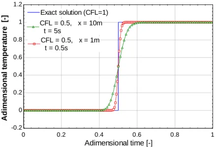
Figure 2 illustrates the numerical diffusion of the upwind scheme: in the case of a temperature step applied at the inlet of a pipe at initial time, it can be noticed that the adimensional temperature response at the pipe outlet is function of the CFL value. When CFL is lower than 1, the numerical

4

diffusion appears: the adimensional temperature increases before the exact solution but reaches the final temperature after the exact solution. The more the CFL value is low, the more the temperature begins to increase soon and the more the temperature reaches the final temperature later.

Figure 2. The numerical diffusion due to CFL conditions for a step input for several CFL conditions.

Notice that for a fixed fluid velocity, the time step is directly linked to the spatial discretisation to ensure convergence. For a fixed CFL value, here 0.5, Figure 3 shows the influence of the spatial and time discretization due to the numerical diffusion. Of course, the solution is closer to the exact solution for higher spatial and time discretization but it involves a more important computational time which could be not compatible with predictive control especially for large networks as studied here.

Figure 3. The numerical diffusion due to CFL conditions equal to 0.5 for varied spatial/time steps.

Various numerical alternatives to reduce the numerical diffusion of the upwind scheme are available in the literature, such as second or higher order upwind schemes [15–18], but they are not be studied herein because they can introduce oscillations or convergence issue once implemented, especially when the spatial discretization is high, i.e. the number of variables is high. To conclude this discussion of finite volume method, notice that it can be extended to two or three dimensions.

0 0.2 0.4 0.6 0.8 1 -0.2 0 0.2 0.4 0.6 0.8 1 1.2 Adimensional time [-] A d im e n s io n a l te m p e ra tu re [-] CFL = 1, Exact solution CFL = 1, Exact solution CFL = 0.5 CFL = 0.5 CFL =0.25 CFL =0.25 CFL = 0.8 CFL = 0.8 0 0.2 0.4 0.6 0.8 1 -0.2 0 0.2 0.4 0.6 0.8 1 1.2 Adimensional time [-] A d im e n s io n a l te m p e ra tu re

[-] Exact solution (CFL=1)Exact solution (CFL=1) CFL = 0.5, Dx = 10m Dt = 5s CFL = 0.5, Dx = 10m Dt = 5s CFL = 0.5, Dx = 1m Dt = 0.5s CFL = 0.5, Dx = 1m Dt = 0.5s

5

To avoid being subjected to numerical diffusion, an alternative modelling method based on the standard TRNSYS Type 31 component is proposed. For further information about the original model, the reader can refer to [8,19]. This modelling method is based on a Lagrangian approach, i.e. the properties of each fluid particle are considered along their direction in function of time, considering the energy balance in each cell. In this approach, the momentum balance is neglected and the fluid is considered as incompressible, so the mass and energy balance are expressed by:

, (9)

̇, (10)

This component models the thermal behaviour of fluid flow in a pipe whose cell volume and density are considered as constant. That is valid for low temperature variation of a fluid cell covering the pipe which occurs in an insulated pipe as the studied case. This assumption involves a constant density. The pipe is divided in cells that follow the heat waves propagation: the entering fluid shifts the position of the existing cell and the energy balance is applied to each cell.

3. Methodology

In order to simplify the resolution, the flow was considered as incompressible which is valid if the fluid is water and for low pressure variations [20]. To simplify and show the limitations of each investigated method, an adiabatic pipe is considered in the first part of this study. A temperature profile is applied at the pipe inlet and the pipe outlet is analysed.

The main approach investigated is the one-dimensional finite volume method developed and available under Modelica platform. This software is particularly adapted to solve transient complex systems (thermal, mechanical, …) and a lot of components are already available that can be interconnected by a graphical interface. Here a validated library called Thermocycle [21] is used to solve the transient problem.

A bi-dimensional modelling of the pipe is considered as the reference case of the studied flow problem. It takes place under OpenFoam platform. A turbulence model k-ε is considered and the natural convection influence is neglected to consider the case as axisymmetric while high Reynolds number are studied (between 105 and 106). The turbulence intensity, the turbulent Prandtl number and the turbulent to molecular viscosity ratio can be calculated by [22–24]. This bi-dimensional modelling method involves a radial velocity and temperature profile in the pipe. This method is called “2D finite volume method”.

The third approach considered is the Lagrangian approach explained in the previous section which is called “plug flow”. It is assumed that there is no pressure loss into the cells to simplify the equation system resolution. However, due to the pipe length of DHN parts, it is proposed to set a pressure loss only at the pipe outlet to consider the pump work. This pressure loss is defined by the non-linear Darcy-Weisbach equation [25]. This assumption is also implemented in the one-dimensional finite volume method to consider the pressure loss at the outlet pipe.

To anticipate the discussion results, the others physical phenomenon occurring in a pipe, i.e. the heat losses and the pipe inertia influences, are introduced. The constituting pipe material itself is divided into cells initialized to a fixed temperature. Each cell has a thermal inertia (TI) depending of the geometrical characteristic of the pipe:

, (1)

where V is the cell volume [m³] is defined as ( ) and where and are respectively the density [kg/m³] and the specific heat [J/kg/K] of the constituting material of the pipe and Dout and

Din respectively the outer and inner pipe diameter [m].

The heat exchanges between the fluid cell and the constituting pipe cell or between the constituting pipe cell and the ambient are computed by using heat transfer coefficient. The heat transfer coefficient corresponding to the heat exchange between the fluid and the pipe can be computed

6

from the flow characteristics by [26]. The present contribution is not intended to be a review of the literature on the calculation of heat losses and thermal resistance in district heating and the interested reader is referred to [15, 16] for a more complete information concerning the heat transfer between the pipe and the ambient. Herein, previous experimental studies are used to determine the heat loss coefficient of the pipe [27,28].

4. Results and discussion

4.1 Introduction

To support the discussion, a typical district heating application available on the University campus in Liège is used. The installed network has a total length of 10 km and distributes pressurized hot water to approximately 70 buildings located in the University campus representing a total heated area of about 470000 m². Buildings are very different in nature namely, classrooms, administrative offices, research centers, laboratories and a hospital. The effective peak power of the network is around 56MW for a total of 60000 MWh per year. Heat losses represent approximately 10% of the annual energy supplied to the DHN.

The district heating network is divided into twenty-three sections having the same geometric characteristic but pipe diameters ranging from 50 to 350 mm. The insulation used is mineral wool with an identified thermal conductivity of 0,047 W/m/K. The insulation thickness varies between 80 and 130 mm. Mass flow rate range in the biggest pipes (0.35m of diameter) is between 50 to 200 kg/s corresponding to a velocity range of 0.4 to 1.8 m/s.

In this study, a pipe of 0.35m of diameter (the main pipes of the network which ensure the main part of the heat transport) is considered and the corresponding heat transfer coefficient was previously identified [27] at the value of 0.76 W/m²/K.

First, an adiabatic pipe of 20 meters is investigated in which a velocity of 1m/s is considered, which is close to the annual average velocity of the DHN studied. The temperature profile at the inlet pipe is a “step” of 10K from 323K to 333K in 10s. It is approximated by the first part of a sinus which approaches a temperature increase in a DHN (see Figure 4 plain line).

4.2 Adiabatic case study

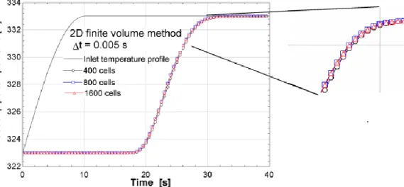
The first results concern the spatial discretization of the 2D finite volume method: 400, 800 and 1600 cells are investigated corresponding to a = 5, 2.5 and 1.25 cm. Doing so, the accuracy level can be identified as a function of the spatial discretisation. Here, the outlet temperature, drawn in the following figures dedicated to 2D finite volume method, is the average temperature of 40 equidistant check points on the radial axis from the pipe centre to the wall to consider the outlet temperature profile.

Figure 4. 2D finite volume results for several spatial discretizations to determine the accuracy level.

7

The increased cell number from 400 (black dots) to 800 cells (blue squares) does not involve a significantly higher accuracy level: the outlet pipe temperature results do not change a lot (Figure 4). This is particularly true when the cell number grows from 800 to 1600 cells (red triangles) where the results are quasi identical. Therefore for the first spatial discretization considered, the solution of this bi-dimensional finite volume method can be considered reliable.

Figure 5, the comparison results of the 1D finite volume method (blue circles) and the 2D finite volume method (black squares) is drawn for a same spatial discretization (400 cells): the outlet pipe temperature response follows the same trend in both cases. In this case, the numerical diffusion occurs, CFL value is 0.5, so the 1D finite volume method “acts” like the more accurate bi-dimensional simulations where a velocity profile in the pipe is considered. However, for the exact solution of the 1D finite volume method problem (red straight line in Figure 5), the increase of the temperature appears a little bit later than the 2D finite volume method but then, the temperature outlet follows the trend of the 2D finite volume method. It is due to the fact that the model is only one-dimensional and does not consider a radial velocity profile involving a higher velocity in the pipe centre, and therefore, quicker heat propagation. However the difference of the temperature outlet between these two methods is quite limited and the actual behaviour is correctly assessed.

Figure 5. Comparison of the 2D and 1D finite volume method for a same spatial discretization.

Despite the fact that the 1D finite volume method assesses the trend of the outlet pipe temperature as the 2D finite volume method for an important spatial discretization, an issue appears with the use of the one-dimensional finite volume method available under Modelica platform. When the pipe length increases, the number of cells and the variable number increases. It leads to a higher computational time cost (second order). However beyond about 50 meters the software does not converge anymore. If the spatial discretization is reduced (from 0.05 m to 0.1 m by cell), this issue occurs for a higher pipe length: about 100 meters. It is supposed that this issue could come from the higher variables number whose orders of magnitude are very different. While the aim of this study is to model large network, it is proposed to decrease the spatial discretization. Unfortunately, if the spatial discretization is reduced to allow the resolution of the equation system of longer pipes, the numerical diffusion appears more significantly than before and leading to a dispersion of the outlet pipe temperature as it is shown in Figure 6:

8

Figure 6.The influence of the numerical diffusion on the outlet pipe temperature for the twenty meters pipe.

Nevertheless, the influence of the numerical diffusion on the outlet temperature for a twenty meters pipe is quite limited: the temperature increase occurs about four seconds sooner and the temperature reaches the maximal value about four seconds later. The case of a one kilometre pipe, which makes the university network up, is studied: the reader can notice in Figure 7 the significant influence on the outlet temperature due to the numerical diffusion. Indeed the rise of the temperature pipe outlet can occur very soon (up to about 600 seconds earlier if the spatial step is of 100 meters) compared to the exact solution (black straight line).

Figure 7.The influence of the numerical diffusion on the outlet pipe temperature for one thousand meter pipe.

Generally in the DHN Modelica model found in the literature [21,29], the spatial discretization is very poor, typically 2 or 3 cells for several dozens of meters, a priori, to allow the convergence of these complex model. However this spatial discretization leads to a lack of precision in the results as it was previously shown. While the aim of this article is to assess the temperatures at some key locations to perform a control of the network, the 1D finite volume method available in Modelica is not suitable to reach this aim. Moreover these two first approaches need important computational time due to the spatial discretization considered. This characteristic reinforced the fact that these approaches are not suitable for their use coupled to a predictive control.

9

The results of the “plug flow” model are drawn in Figure 8: the exact solution of the one-dimensional finite volume method (black dots) is found with the plug flow model with spatial discretization of one meter (blue dots line). If the spatial discretization is more refine, 0.5 m, the exact solution of the 1D finite volume method is found too (red line) without numerical diffusion. In the opposite case, if the spatial discretisation is rougher, 2 m, discontinuities are noticed in the results due to the lower spatial discretization. In this last case, there are not enough cells to describe correctly the fluctuations of the inlet pipe temperature. The “plug flow” model allows a quicker resolution of the system by a factor 103compared to the resolution of 1D finite volume method. From now, this model is the only one to be investigated to consider the heat losses and the thermal inertia of the pipe influence.

Figure 8. Plug flow results for several spatial discretization.

4.3 Influence of the heat losses and pipe thermal inertia

Since the “plug flow” model can assess the exact solution of the 1D finite volume pipe problem, the model is extended to catch the physical behaviour of a real network, i.e. the ambient losses and the thermal inertia of the pipe. While the length of pipes can reach several kilometres, the ambient losses have an influence on the temperature. In a previous study [27], these annual losses were identified at about 10% of the annual heat supplied for the district heating network studied. It is the same order of magnitude that found in others studies [30–32] but notice that these losses can reach 20% of the annual heat supplied [31]. On the other hand, the thermal inertia of the pipes should be also considered. Indeed it induces a delay in the heat transport: when the fluid temperature increases (respectively decreases) in the pipe, there is a delay of the increase (respectively the decrease) temperature at the outlet pipe while the pipe is heated (resp. releases heat). This effect is more important when the thickness of the pipe increases especially if the pipe is in a metal constituting material, which is generally the case for large district heating networks.

A pipe of one thousand meters is considered to see the influence of the heat losses1. Indeed, for small pipe length, the heat losses have no significant influence on the outlet temperature since the pipe is insulated. In this case the ambient temperature is taken equal to 293 K. The influence of the thermal inertia of the pipe is considered with a pipe thickness of 0 cm (no thermal inertia) and 1 cm (a conventional thickness for the pipe diameter considered).

Figure 9 shows that the outlet temperature pipe begins to slightly decrease due to the heat. Since the velocity is 1 m/s, this temperature decrease takes one thousand seconds to appear at the outlet and is worth 0.1 K. Then the outlet temperature increases due to the temperature “step” at the inlet.

1

For the pipe length and for the heat losses coefficient considered in this study until now, the impact on the outlet pipe temperature is very tiny < 0.01°K. The pipe length considered here is therefore proposed longer.

10

However the temperature increase is slower when the thermal inertia is considered (red dashed line) while the pipe is heated up. Indeed, the thermal inertia induces a significant delay on the thermal response: the time required for the temperature to reach the steady state level is about 200 seconds (blue dots line) instead of 10 seconds when the pipe inertia is not considered. Of course in the case of a temperature decrease, the delay also exists due to the release of the heat inside the pipe.

Figure 9. Heat losses and pipe inertia influences on outlet pipe temperature for the plug flow modelling.

Through these results, the significant influence of the pipe thermal inertia on the heat transport in pipes is demonstrated. Indeed for more complex and longer network this delay has to be considered during the early morning heating boost for example. To guarantee the thermal comfort of the users, this heating boost is generally performed too soon leading to more important and useless heat losses. Coupled to a predictive control of energetic needs of buildings, it could be possible to feed only the required heat demand in the network.

5. Conclusions

A comparison between several modelling methods is performed to determine the most convenient way to model the heat transport in large district heating networks to improve their control at low cost, i.e. by model the DHN behaviour instead of their costly instrumentation.

First, an adiabatic pipe is considered to show the limitations of each modelling method investigated and an existing district heating network is used to determine the main parameters of the study. For the same spatial discretization, the bi-dimensional finite volume model does not bring substantial details in the results (i.e. the outlet temperature of the pipe) compared to a one-dimensional finite volume modelling. However to get reliable results, spatial discretization of the pipe is important, as it involves a high computational time incompatible with the final use of this model, namely the predictive control. On the other hand, the decrease in the spatial discretization level involves a significant numerical diffusion linked to the discretization scheme used, and therefore an anticipation of the heat waves at the pipe outlet. Finally, the use of one-dimensional modelling is restricted by a non-convergence issue appearing when the length of the pipes, and so the variable number, increases. The authors suppose that it could be due to the numerous variables whose the order of magnitudes are very different causing inconstancy in the resolution method. An alternative method should be to assume that the density is constant in this model while the heat losses of the pipe and so temperature variations are reduced to simplify the equations system.

The results of the “plug flow” model give us the same accuracy than the exact solution of the one-dimensional problem model. Moreover, these results are obtained with a rough spatial discretisation

11

leading to a very quick simulation. Since the “plug flow” results of the adiabatic case are equal to the exact solution of the one-dimensional finite volume problem, heat losses and pipe thermal inertia influences are also considered. For an insulated pipe, the heat losses have a slight influence on the outlet temperature of the pipe especially for short pipe length. However, they have to be considered while they generally represent 10% of the heat supplied to the network. On the other hand, the influence of the thermal inertia of the pipe on the outlet pipe temperature has been exhibited as this induces a significant delay in the heat transport.

This final model will serve in the future work dedicated to assess the behaviour of a complete heat district network. Once validated, a control will be implemented to reduce the heat consumption of the district network and to assess the economic and environmental benefits.

Nomenclature

A heat exchange area, m² Cp specific heat, J/(kg K)

D diameter, m

.

m mass flow rate, kg/s

p pressure, Pa ̇ heat flux, J/s t time, s T temperature, K u velocity, m/s V volume, m³ Greek symbols ρ density, kg/m³ Abbreviations

DHN, District heating network FVM, Finite volume method

in inner out outer * adjacent cell

References

1. Rezaie B, Rosen MA. District heating and cooling: Review of technology and potential enhancements. Appl Energy. 2012;93:2–10.

2. Dobos L, Abonyi J. Controller tuning of district heating networks using experiment design techniques. Energy. 2011;36:4633–9.

3. Wissner M. Regulation of district-heating systems. Util Policy . 2014 Dec;31(0):63–73. 4. MOEK. Infrastructure monopoly of the Moscow government in heat energy distribution. p.

1–15.

5. Madsen H, Sejling K, Søgaard HT, Palsson OP. On flow and supply temperature control in district heating systems. Heat Recover Syst CHP. 1994 Nov;14(6):613–20.

6. Laajalehto T, Kuosa M, Mäkilä T, Lampinen M, Lahdelma R. Energy efficiency

improvements utilising mass flow control and a ring topology in a district heating network. Appl Therm Eng . 2014 Aug;69(1–2):86–95.

7. Jie P, Zhu N, Li D. Operation optimization of existing district heating systems. Appl Therm Eng. 2015 Mar 5;78(0):278–88.

12

9. Gabrielaitienė I, Kačianauskas B, Sunden B. Application of the Finite Element Method for Modelling of District Heating Network. J Civ Eng Manag. 2003;9(3):153–62.

10. Patankar S. Numerical heat transfer and fluid flow. Series in coputational methods in mechanics and thermal sciences. 1980. p. 1–197.

11. Tannehill JC, Anderson DA, Pletcher RH. Computational Fluid Mechanics and Heat

Transfer. Computational and Physical Processes in Mechanics and Thermal Sciences. 1997. 12. Quoilin S, Bell I, Desideri A, Dewallef P, Lemort V. Methods to Increase the Robustness of

Finite-Volume Flow Models in Thermodynamic Systems. energies. 2014;7:1621–40. 13. Courant R, Friedrichs K, Lewy H. Über die partiellen Differenzgleichungen der

mathematischen Physik. Math Ann . 1928;100.

14. Zurigat YH, Ghajar AJ. COMPARATIVE STUDY OF WEIGHTED UPWIND AND SECOND ORDER UPWIND DIFFERENCE SCHEMES. Numer Heat Transf Part B Fundam. 1990;18:61–80.

15. Lai C, Bodvarsson G. A second-order Upwind Differencing Method for Convection-Diffusions equations. Earth Sci Div Annu Rep. 1986;93–7.

16. Patel MK, Markatos NC, M. C. Method of reducing false-diffusion errors in convection – diffusion problems. Cent Numer Process Anal. 1985;

17. Tolstykh AI, Lipavskii M V. On Performance of Methods with Third- and Fifth-Order Compact Upwind Differencing. J Comput Phys . 1998;140:205–32.

18. Stevanovic VD, Jovanovic ZL. A hybrid method for the numerical prediction of enthalpy transport in fluid flow. International Communications in Heat and Mass Transfer. 2000. p. 23–34.

19. TRNSYS 17 Manual – Volume 4 – Mathematical Reference.

20. Hoffman J, Johnson C. Computational Turbulent Incompressible Flow. 2007;4:415.

21. Wetter M, Zuo W, Nouidui TS, Pang X. Modelica Buildings library. J Build Perform Simul . 2014;7:253–70. Available from:

22. Compass. Turbulence Handbook, Environment for Multi-Physics simulation, including Fluid Dynamics, Turbulence, Heat Transfer, Advection of Species, Structural mechanics, Free surface and user defined PDE solvers.

23. Guidelines for Specification of Turbulence at Inflow Boundaries [Internet]. [cited 2014 Jan 12]. Available from: http://support.esi-cfd.com/esi-users/turb_parameters/

24. Basim O. Hasan. Turbulent Prandtl Number and its Use in Prediction of Heat Transfer Coefficient for Liquids. Coll Eng J. 2007;10:53–64.

25. Krope A, Krope J, Ticar I. The reduction of Pipelines, friction losses in district-heating. J Mech Eng. 2000;46(8):525–31.

26. Nellis GF, Klein SA. Heat transfer. Press CU, editor. 2009.

27. Sartor K, Quoilin S, Dewallef P. Simulation and optimization of a CHP biomass plant and district heating network. Appl Energy. Elsevier Ltd; 2014;130:474–83.

28. Gary EP, Marlin JK, David LCLFm. Field Measurements of Heat Losses from Three Types of Heat Distribution Systems. 1991.

29. Nytsch-Geusen C. Buildingsystems - A Modelica-library for modelling and simulation of complex energetic building systems [Internet]. [cited 2014 Jan 12]. Available from: http://www.modelica-buildingsystems.de/library/overview.html

30. Kemal Çomaklı, Bedri Yüksel ÖÇ. Evaluation of energy and exergy losses in district heating network. Appl Therm Eng. 2004;24(7):1009–17.

31. Frederiksen S, Werner S. Fjärrvärme : Teori, teknik och funktion. Press L, editor. 1993. 32. Hlebnikov A, Siirde A. The major characteristic parameters of the Estonian district heating