HAL Id: hal-00329150
https://hal.archives-ouvertes.fr/hal-00329150
Submitted on 1 Jan 1999
HAL is a multi-disciplinary open access
archive for the deposit and dissemination of sci-entific research documents, whether they are pub-lished or not. The documents may come from teaching and research institutions in France or abroad, or from public or private research centers.
L’archive ouverte pluridisciplinaire HAL, est destinée au dépôt et à la diffusion de documents scientifiques de niveau recherche, publiés ou non, émanant des établissements d’enseignement et de recherche français ou étrangers, des laboratoires publics ou privés.
energy spectra from the Equator-S ion composition
(ESIC) instrument
L. M. Kistler, B. Klecker, V. K. Jordanova, E. Möbius, M. A. Popecki, D.
Patel, J. A. Sauvaud, H. Rème, A. M. Di Lellis, A. Korth, et al.
To cite this version:
L. M. Kistler, B. Klecker, V. K. Jordanova, E. Möbius, M. A. Popecki, et al.. Testing electric field models using ring current ion energy spectra from the Equator-S ion composition (ESIC) instrument. Annales Geophysicae, European Geosciences Union, 1999, 17 (12), pp.1611-1621. �hal-00329150�
1Space Science Center, Morse Hall, University of New Hampshire, Durham, NH, USA
E-mail: [email protected]
2Max-Planck-Institut fuÈr Extraterrestriche Physik, Garching, Germany 3C.E.S.R.., Toulouse, France
4I.F.S.I, Rome, Italy
5Max-Planck-Institut fuÈr Aeronomie, Katlinberg-Lindau, Germany 6University of Washington, Seattle, WA, USA
7Swedish Institute of Space Physics, Kiruna, Sweden 8University of California, Berkeley, CA, USA
Received: 26 March 1999 / Revised: 9 August 1999 / Accepted: 17 August 1999
Abstract. During the main and early recovery phase of a geomagnetic storm on February 18, 1998, the Equa-tor-S ion composition instrument (ESIC) observed spectral features which typically represent the dieren-ces in loss along the drift path in the energy range (5±15 keV/e) where the drift changes from being E ´ B dominated to being gradient and curvature drift dominated. We compare the expected energy spectra modeled using a Volland-Stern electric ®eld and a Weimer electric ®eld, assuming charge exchange along the drift path, with the observed energy spectra for H+
and O+. We ®nd that using the Weimer electric ®eld
gives much better agreement with the spectral features, and with the observed losses. Neither model, however, accurately predicts the energies of the observed minima. Key words. Magnetospheric physics (energetic particles trapped; plasma convection; storms and substorms)
1 Introduction
During geomagnetic storms, the ion energy spectra in the ring current show minima which re¯ect the drift history of the ion population. Over the energy range from 1 to 50 keV/e, the dominant drift changes from the eastward and sunward E ´ B drift at low energies, to the westward gradient and curvature drifts at higher energies. In the energy range where the two contribu-tions are approximately equal, the drifts are very
sensitive to the exact electric and magnetic ®eld con®gurations. The ion spectra observed on the dayside typically contain one or more minima which correspond to the drift paths on which the greatest losses occur, either because they have the longest drift time, or because they drift the closest to the Earth, where losses are greater. Many studies (e.g., Kistler et al., 1989; Fok et al., 1996; Jordanova et al., 1999) have shown quali-tative agreement between observed and predicted spec-tra based on these principles. However, there has been diculty in getting quantitative agreement. The reason for this is most likely that the electric and magnetic ®elds used for modeling the spectra have been simpli®ed.
The most common electric ®eld used for this type of modeling is the Volland-Stern (Volland, 1973; Stern, 1975) electric ®eld. The Volland-Stern ®eld is derived from the potential:
Uconv ARcosin u 1
where Ro is the radial distance in the equatorial plane, c
is an adjustable shielding parameter, normally taken to be 2, u is the azimuthal angle, measured eastward from midnight, and A gives the magnitude. Maynard and Chen (1975) determined an empirical formula for A as a function of the planetary index Kp, for the c 2 case. This ®eld has the advantage of being analytically very simple, and therefore easy to use in numerical models. However, recent measurements indicate that it may be very far o from the actual electric ®eld, particularly during storm times (Wygant et al., 1998). A more recent model with a much stronger empirical basis is the Weimer model (Weimer, 1995, 1996). This model is based on measurements of the electric potential by the vector electric ®eld instrument on the DE2 spacecraft. The data were sorted into groups by IMF clock angle, IMF magnitude and dipole tilt angle, and then the
measurements from each group were used to derive a model in terms of a spherical harmonic expansion. By using the measured IMF parameters, this model can be used to give a time dependent estimate of the electric ®eld. The model gives the potential at low altitudes. This potential must then be mapped up the ®eld line to get the equatorial electric ®eld.
In this work, we show one example of a geomagnetic storm where large ¯ux enhancements were observed in the ring current. The energy spectra as observed with the Equator-S ion composition (ESIC) instrument showed the features that result from losses along drift paths. We will use both the Volland-Stern and the Weimer electric ®elds combined with a dipole magnetic ®eld to deter-mine the drift trajectories of ions during a geomagnetic storm. We will then determine the expected energy spectra on the dayside, assuming that charge exchange is the only loss process, and compare the expected energy spectra with those observed.
2 Instrumentation
The Equator-S satellite is in a highly elliptical orbit, with an apogee of 11.3 Re and a perigee of 500 km. It orbits in the geographic equatorial plane. The initial apogee was at 11:00 LT, and it then precesses toward earlier local times. The data shown here are mainly from the Equator-S ion composition instrument (ESIC). ESIC measures the 3-dimensional distribution functions of the major ion species in the magnetosphere and magneto-sheath over the energy per charge range 20±40000 eV/e. It is a combination of a top-hat electrostatic analyzer followed by post-acceleration by 15±18 kV and a time-of-¯ight measurement. It is similar to the CODIF (CIS1) instrument designed for CLUSTER (ReÁme et al., 1997) and the TEAMS instrument on FAST (MoÈbius et al., 1998). It can resolve the major ion species, H+, He++,
He+and O+.
The electrostatic analyzer is divided into two halves, with geometric factors dierent by a factor of 100. Only one half operates at a time, giving a 180° instantaneous ®eld of view divided into eight sectors of 22.5° each. The full 3D distribution is achieved using the spin. The electrostatic analyzer sweeps through the full energy range 16 times per spin, so that the full distribution is obtained in one spin.
An on-board processor collects the event data from the sensor and classi®es each event by mass, energy, and angle. It then bins the data and creates ``data products'' which consist of 3-dimensional (3D) distributions, a mass spectrum, and moments of the distribution. In addition products containing the raw count rates from the sensor and a sample of raw data from individual ions, including the time-of-¯ight, position, spin sector, and energy step are also generated to monitor the performance and calibration of the sensor. These 3D distribution products are available for each of the four major species, H+, O+, He++, and He+, with either 16
or 32 energy bins, and 88, 24, or 12 angular bins. For the mass spectrum, the mass space from 0 to 70 AMU is
divided into 31 bins spaced as the square-root of the mass, with a factor of four discontinuity at 9 AMU. This product allows minor species such as O++ to be
detected, and is also useful for determining the rate of background in the instrument, as will be illustrated. The combination of products obtained at any time and their time resolution depends on the telemetry rate and the expected count rates for the particular species in the measurement region.
During the time period of interest, the satellite was moving from L = 8 to L = 4. At L = 4, the satellite is in the radiation belts. Because this instrument requires a coincidence for a measurement, it is less susceptible to background from penetrating particles than an instru-ment relying on singles rates. However, when the background rate is high enough, false coincidences are observed. These can appear with equal probability at any time-of-¯ight. Because the real ions occur as peaks in time-of-¯ight for a particular energy, they can be easily distinguished from the background if their count rate is suciently high.
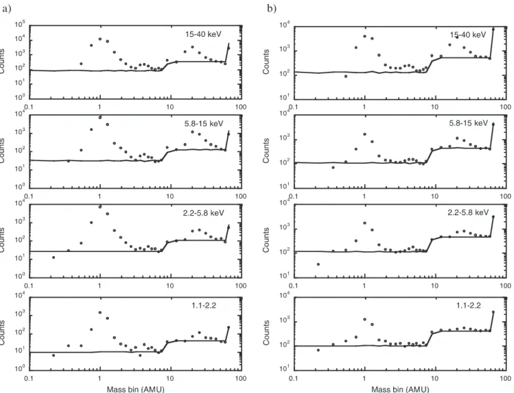
To illustrate the eect of background, Fig. 1a shows mass spectra from the instrument for the top four energy steps of the mass spectrum product. These correspond to energies 15±40 keV/e, 5.8±15 keV/e, 2.2±5.8 keV/e and 1.1±2.2 keV/e. Note that the mass spectrum has much wider energy bands (by a factor of four) than the 3D distribution functions which are used to determine the energy spectra. Because the energy steps are being combined, the mass resolution appears worse than it is. The time period shown is when the spacecraft is at L = 5.75 during an inbound pass on February 18, 1998. The background level is indicated with a solid line. The peaks for H+, He+ and O+ are clearly visible and
distinguishable from background. At the lowest energy, the O+peak is still a factor of four above background.
Figure 1b shows the mass spectra for a later time period, when the satellite is at L = 4.25 Re, and has entered the outer radiation belt, where penetrating energetic elec-trons cause background in the instrument. At high energies, the peaks for the individual ions are still clearly visible. At lower energies, the proton peak is still signi®cantly above background, but the other species are background dominated. Here we will concentrate on observations of H+ and O+, the dominant species,
limiting the O+ data to where it is well above
background. 3 Observations
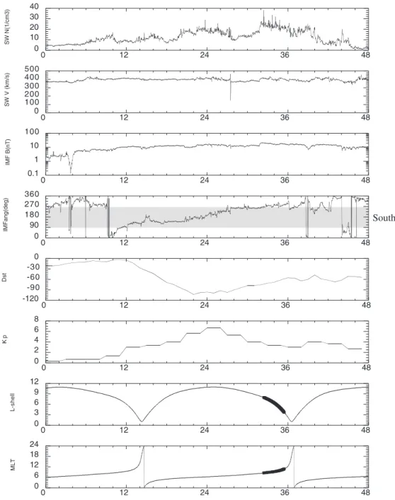
On February 17±18, 1998, a geomagnetic storm with a minimum Dst of )103 occurred. The top four panels of Fig. 2 show the solar wind proton density, N, and speed, V, the interplanetary magnetic ®eld magnitude, B, and clock angle from the Wind spacecraft. The clock angle is measured from the Z axis in the Y-Z gsm plane. The time scale has been shifted by one hour to allow for features observed at the Wind location to reach the Earth. From hour 12 to hour 28, the IMF had a southward component, rotating 180° from +Y GSM,
southward, around to )Y GSM. For the next 8 h, the IMF remained in the )Y direction with a small Z component, sometimes north, sometimes south. Panels 5 and 6 show the Dst and Kp pro®les, respectively. The magnetosphere clearly responded to the southward IMF with a large drop in Dst and an increase in Kp. The peak of the main phase of the storm occurred at around 00 UT on February 18. Panels 7 and 8 show the L-value and magnetic local time of the Equator-S spacecraft. The portion of the Equator-S orbit of interest is given by the heavy line. During this time, Equator-S was moving inbound from L = 8 to L = 4 in the pre-noon local time sector. This is the optimum sector for observing the drift eects on the energy spectra.
Figure 3 shows energy time spectrograms of H+and
O+ from 8:00±11:30, when the spacecraft is moving
from L = 8.3 to L = 4.0. As the spacecraft moves inbound, a minimum is observed below about 10 keV. The width in energy of the minimum increases as the spacecraft moves inbound. A second minimum below about 4 keV is also evident in the protons. The large ¯ux observed below 2 keV in O+ after 10:45 is due to the
penetrating electron background. This masks whether the second minimum is also observed in O+. To show
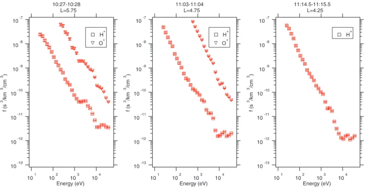
the features more quantitatively, Fig. 4 gives the omni-directional distribution function, f, as a function of energy for H+ and O+ for one-minute time periods
corresponding to L = 5.75, 4.75, and for H+ at
L = 4.25. Note that because f is a function in velocity, and not in energy, O+ has a higher value in f although
its ¯ux is lower. At L = 5.75, both H+ and O+ have
two minima at about 2 keV and 10 keV. At L = 4.75, the lower energy minimum is just a slight in¯ection in the curve, and there are now two high energy minima for H+, at 10 and 20 keV. The same approximate features
are observed at L = 4.25. Finally, Fig. 5a±c show pitch angle distributions corresponding to L = 5.5±6.0, and L = 4.5±5.0 for H+and O+and L = 4.0±4.5 for H+.
The longer time average was used to increase statistics. At L = 5.5±6.0, the high energy distributions are peaked at 90° pitch angle. At 10.7 keV, the approximate energy of a minimum, a ``head-and-shoulders'' distribu-tion is observed. Finally, at the low energy minimum, there is a minimum at 90° pitch angle. The O+ Fig. 1. a Mass distributions at L = 5.75 for four energy ranges. The solid line gives the background level. The jump in background observed at 9 AMU is due to a discontinuity in the mass algorithm. b Mass distributions at L = 4.25 in the same format as a
distributions are similar to those of H+. At lower
L-values the high and low energy distributions are more isotropic, except for the loss cone. In Fig. 5b, the H+
distribution at 10 keV is strongly peaked at 90° while the O+ is more isotropic.
4 Modeling
The energy spectra and pitch angle distributions ob-served can be used to test models of the magnetospheric convection electric ®eld. To do this we start at the spacecraft location, and model the ion bounce averaged drift paths backwards for 24 h or until the ion reaches L = 10. Assuming that charge exchange is the only loss
mechanism, we calculate the loss to the distribution function as the ion drifts from the tail to the observation location. Then we assume an initial power law distribu-tion, normalized to the observed spectrum, and calculate the eect that the losses would have on that spectrum. These can then be compared with the observations.
We model the bounce averaged drift paths for two ®eld models: a dipole magnetic ®eld combined with the Volland-Stern electric ®eld, and a dipole magnetic ®eld combined with the Weimer electric ®eld. Both electric ®elds are time-dependent. The Volland-Stern model is parametrized by Kp. We use the observed Kp values during the storm to change the magnitude of the electric ®eld as a function of time. Since the Kp is available for 3-h time periods, we linearly interpolate between t3-he
Fig. 2. Solar wind and magnetic ®eld parameters from the MFI and SWE instruments on the Wind spacecraft, Dst and Kp indices, and L-shell and magne-tic local time for the Equator-S spacecraft. The Wind parameters have been shifted in time by one hour
dierent Kp levels, which results in a slow time varia-tion. The Weimer electric ®eld is parametrized by the solar wind speed, the IMF direction, and the dipole tilt. We have used values from MFI and SWE instruments on the Wind spacecraft, assuming a travel time of 1-h. In this case the values are updated every 5 min, so the time variation is much faster.
Figure 6 shows the drift paths of the ions which are observed at L = 5.75, and 9.57 MLT. The paths are shown for six energies from 35.8 keV down to 3.2 keV. The distance between the symbols indicates 1 hour of
drift time. Figure 6a±c is for the Volland-Stern electric ®eld for three dierent pitch angles, and Fig. 6d±f for the Weimer electric ®eld for the same pitch angles. One obvious dierence is that the Volland-Stern drift paths are much more regular. This is due to both the simple analytical form of the ®eld, and the slower time variation. For drifts in the Volland-Stern electric ®eld, the transition region between eastward and westward drifting paths is between 3 and 5 keV. For the Weimer electric ®eld, the transition energy is a little higher, particularly at the smaller pitch angles. At 45° and 10°,
Fig. 3. Energy-time spectro-grams for H+and O+for a time
period on February 18, 1998, when Equator-S was moving inbound from L = 8.3 to L = 4.0 in the pre-noon local time sector
Fig. 4. Ion distribution function versus energy for 1-min time periods at L = 5.75, L = 4.75, and L = 4.25. O+is not shown at L = 4.25
the transition energy is between 8 and 13 keV. Another dierence is that the eastward drift in the Weimer ®eld is signi®cantly slower than in the Volland-Stern ®eld (compare the 3.2 keV path in all cases). Finally, the
westward Volland-Stern drift paths tend to go closer to the Earth than the Weimer paths. For both ®elds, the transition energy is higher at lower pitch angles. This can lead to the ``head and shoulders'' type pitch angle
Fig. 6a±f. Bounce averaged drift paths for ions which arrive at L = 5.75, 9.57 MLT with 6 dierent energies. The paths were calculated using a dipole magnetic ®eld and either a Volland-Stern electric ®eld (a±c) or a Weimer electric ®eld (d±f). The legend gives the ion energy in keV Fig. 5. a Pitch angle distributions at three dierent energies for H+
and O+at L = 5.5±6.0. The dierent symbols represent dierent look
directions with respect to the spin axis in the instrument. b Pitch angle distributions at three dierent energies for H+and O+at L = 4.5±
5.0. The dierent symbols represent dierent look directions with
respect to the spin axis in the instrument. c Pitch angle distributions at three dierent energies for H+at L = 4.0±4.5. The dierent symbols
represent dierent look directions with respect to the spin axis in the instrument
distribution observed at 10.7 keV in Fig. 5a if the energy corresponds to the range where the low pitch angle ions drift eastward while the high pitch angle ions drift westward, like the drift path of an 8.4 keV ion in the Weimer model.
Figure 7 compares the drift paths at L = 4.25 and MLT = 10.41. The dierence between the transition energies for this L-value and local time is larger: the transition energy in the Volland-Stern electric ®eld is between 3 and 5 keV, for the 89° pitch angle ions, and between 5 and 8 keV at lower pitch angles, while for the Weimer ®eld it is between 8 and 13.6 for 89° and 45° pitch angle, and greater than 13.6 for the ions at 10°. Again, the eastward drift in the Weimer ®eld is slower than for the Volland-Stern ®eld.
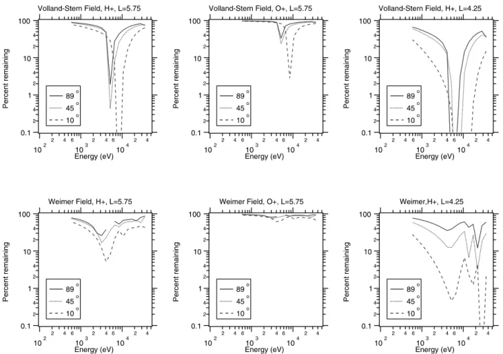
Figure 8 shows the percent of the distribution func-tion that will remain after the ions have drifted in from L = 10. The percent remaining is shown as a function of energy for the two models and for three dierent pitch angles. We have used the charge exchange cross sections given by Smith and Bewtra (1978) with the neutral hydrogen geocorona model of Rairden et al. (1986). H+and O+results at L = 5.75 are shown, and
H+ only at L = 4.25. Using the Volland-Stern electric
®eld gives one deep minimum, which corresponds to the region around the transition energy. Interestingly, the predicted distributions using the Weimer electric ®eld have multiple minima. A broad dip is observed, with its minimum from 3±5 keV (depending on pitch angle). An examination of the drift trajectories in Figs. 6 and 7 shows that this minimum results from the slow eastward drift paths. The Weimer ®eld then produces second and third minima corresponding to the transition energy and above. The highest energy minima result from particular ion energies which make multiple transits around the Earth before reaching the spacecraft location. These types of trajectories would be very sensitive to the time dependence of the ®eld. O+, in general loses less, due to
its smaller cross section for charge exchange at these energies. This is consistent with our observation in Fig. 5b that the the O+ is more isotropic at 10.7 keV,
the energy close to the minimum, than H+, and is also
consistent with the smaller minima observed in the spectra in Fig. 4.
Figure 9 shows a comparison of the measured distribution functions as a function of energy for H+
and O+with the predicted spectra using the two electric
®elds. The predicted spectra are determined by assuming
Fig. 7a±f. Bounce averaged drift paths for ions which arrive at L = 4.25, 10.41 MLT with 6 dierent energies. The paths were calculated using a dipole magnetic ®eld and either a Volland-Stern electric ®eld (a±c) or a Weimer electric ®eld (d±f). The legend gives the ion energy in keV
an initial power law spectrum (a straight line in this log-log representation). Power-law spectra were consistently observed by Kistler et al. (1989) on the night-side during storms, over the energy range 1±50 keV. We then apply the losses as shown in Fig. 8 to these spectra. These comparisons should therefore be used to determine how well the model represents the features in the spectra, but not the overall normalization or slope of the spectra. It is also possible that features result from changes in the input spectrum with time, spatial dierences in the spectrum from the dierent tail regions that contribute to the spectra, or from deviations from a power law that were present in the input tail spectrum. These types of eects would not appear in our ``model'' spectra.
For both input ®elds, we have compared the omni-directional energy spectra with the losses calculated for ions with pitch angles of 10°, 45°, and 89°. Using the Volland-Stern electric ®eld gives too large a loss. When the Weimer electric ®eld is used, the magnitude of the losses is much closer to that observed. The smaller O+
cross section for charge exchange at these energies leads to less pronounced minima in the spectra, as observed. In addition, the Weimer electric ®eld is better for predicting the complexity of the spectra observed. It
predicts a low energy broad minimum, which is observed at about 2 keV, and multiple high energy minima, as are observed. However, the energies of the minima predicted do not quantitatively agree with the observed energies.
As a ®nal test, we have compared the pitch angle distributions observed with those predicted by the model. As noted previously, the head-and-shoulders distributions result from the low pitch angle ions drifting eastward while the high pitch angle ions drift westward. Since our model does not reproduce the energy of this transition quantitatively, it is dicult to do a quantita-tive pitch angle comparison in this region. Therefore, we have restricted our comparisons to energies slightly away from the predicted and observed minima. Fig-ure 10 compares the observed H+ and O+ pitch angle
distributions at L = 4.5±5.0 with the predicted distri-butions using the Volland-Stern electric ®eld (solid line) and the Weimer electric ®eld (dotted line) for four energies. To generate our predicted distributions we have assumed an isotropic distribution injected on the nightside. Both models reproduce the observed distri-butions very well at high energies (28 keV and 13.6 keV) and at low energies (1.2 keV). At 8.4 keV, which is the
Fig. 8. The percent of the distribution that remains, as a function of energy, after the ions have drifted from the tail to the observation location. The top panels assume a convection in a Volland-Stern
electric ®eld, and the bottom panels assume convection in a Weimer electric ®eld. Charge exchange with the neutral hydrogen geocorona is the only loss mechanism assumed
Fig. 9. Comparisons of observed spectra and modeled spectra using the Volland-Stern electric ®eld (top panels) and the Weimer electric ®eld (bottom panels) assuming charge exchange is the only loss mechanism. The symbols show the data, and the lines give the model results
Fig. 10. Comparisons of observed and modeled pitch angle distributions using the Volland-Stern electric ®eld (solid line) and the Weimer electric ®eld (dashed line) assuming an initial isotropic distribution and charge exchange as the only loss mechanism
We have used observations of the ion energy spectra using the Equator-S satellite to test the validity of two models of the storm-time convection electric ®eld. This is the ®rst time that the Weimer model has been tested for its validity in the equatorial plane using drift trajectories. We ®nd that assuming convection in a Volland-Stern electric ®eld with charge exchange as the only loss mechanism results in predicted losses that are larger than observed. This was evident in both the predicted energy spectra and the predicted pitch angle distributions. This is in agreement with the ®ndings of Jordanova et al. (1999) from comparisons with POLAR data. Chen et al. (1998) in comparing simulating pitch angle distributions with CRRES data for higher energy ions (>50 keV/e) found the opposite result. Assuming convection in the Weimer ®eld gives signi®cantly better agreement with the magnitude of the losses observed. From comparisons of the drift paths, this is primarily because the Volland-Stern trajectories in the transition region go much closer to the Earth. The dierences in charge exchange cross sections of H+ and O+at these
energies is observed in the spectra and pitch angle distributions, and is accurately reproduced by the models, con®rming our assumption that charge ex-change is the most signi®cant loss process at these L-values and energies. Thus the quantitative dierences more likely lie in the magnetic and electric ®eld models used. The Weimer ®eld accurately reproduces the complex spectra with multiple minima that are observed during this storm. However, it does not quantitatively predict the energies of the minima.
We have shown that using a more realistic electric ®eld signi®cantly improves the agreement with the observed spectra. In future work, we will also include a more realistic magnetic ®eld, both in calculating the trajectories, and in mapping the Weimer electric poten-tial up the ®eld line to test if this will ®nally give quantitative agreement between the model spectra and the observations.
References
Chen, M. W., J. L. Roeder, J. F. Fennel, L. R. Lyons, and M. Schulz, Simulations of ring current proton pitch angle distribu-tions, J. Geophys. Res., 103, 165, 1998.
Fok, M.-C., T. E. Moore, and M. E. Greenspan, Ring current development during storm main phase, J. Geophys. Res., 101, 15 311, 1996.
Jordanova, V. K., C. J. Farrugia, J. M. Quinn, R. B. Torbert, J. E. Borovsky, R. B. Sheldon, and W. K. Peterson, Simulations of o-equatorial ring current ion spectra measured by Polar for a moderate storm at solar minimum, J. Geophys. Res., 104, 429, 1999.
Kistler, L. M. et al., Energy spectra of the major ion species in the ring current during geomagnetic storms, J. Geophys. Res., 94, 3579, 1989.
Maynard, N. C., and A. J. Chen, Isolated cold plasma regions: observations and their relation to possible production mecha-nisms, J. Geophys. Res., 80, 1009, 1975.
MoÈbius, E., et al., The 3-D plasma distribution function analyzers with time-of-¯ight mass discrimination for CLUSTER, FAST, and Equator-S, measurement techniques for space plasmas: J. Borovsky, R. Pfa, D. Young, Eds., American Geophysical Union, Washington, DC, 243 1998.
Rairden, R. L., L. A. Frank, and J. D. Craven, Geocoronal imaging with Dynamics Explorer, J. Geophys. Res., 91, 13 613, 1986. ReÁme, H., et al., The Cluster ion spectrometry experiment, Space
Sci. Rev., 79, 303±350, 1997.
Smith, P. H., and N. K. Bewtra, Charge exchange lifetimes for ring current ions, Space Sci. Rev., 22, 301, 1978.
Stern, D. P., The motion of a proton in the equatorial magneto-sphere, J. Geophys. Res., 80, 595, 1975.
Volland, H., A semiempirical model of large-scale magnetospheric electric ®elds, J. Geophys. Res., 78, 171, 1973.
Weimer, D. R., Models of high-latitude electric potentials derived with a least error ®t of spherical harmonic coecients, J. Geophys. Res., 100, 19 595, 1995.
Weimer, D. R., A ¯exible, IMF dependent model of high-latitude electric potentials having ``space weather'' applications, Geo-phys. Res. Lett., 23, 2549, 1996.
Wygant, J., D. Rowland, H. J. Singer, M. Temerin, F. Mozer, and M. K. Hudson, Experimental evidence on the role of the large spatial scale electric ®eld in creating the ring current, J. Geophys. Res., 103, 29 527, 1998.