Decision and risk analysis for an air carrier under fuzzy conditions
7
0
0
Texte intégral
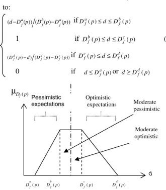
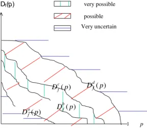
Figure
Documents relatifs