HAL Id: hal-00866077
https://hal.archives-ouvertes.fr/hal-00866077
Submitted on 25 Sep 2013
HAL is a multi-disciplinary open access
archive for the deposit and dissemination of
sci-entific research documents, whether they are
pub-lished or not. The documents may come from
teaching and research institutions in France or
abroad, or from public or private research centers.
L’archive ouverte pluridisciplinaire HAL, est
destinée au dépôt et à la diffusion de documents
scientifiques de niveau recherche, publiés ou non,
émanant des établissements d’enseignement et de
recherche français ou étrangers, des laboratoires
publics ou privés.
A Unified Stochastic Model of Handover Measurement
in Mobile Networks
van Minh Nguyen, Chung Shue Chen, Laurent Thomas
To cite this version:
van Minh Nguyen, Chung Shue Chen, Laurent Thomas. A Unified Stochastic Model of Handover
Mea-surement in Mobile Networks. IEEE/ACM Transactions on Networking, IEEE/ACM, 2013, pp.Page
1-17. �hal-00866077�
A Unified Stochastic Model of Handover
Measurement in Mobile Networks
Van Minh Nguyen, Chung Shue Chen, Member, IEEE, Laurent Thomas
Abstract—Handover measurement is responsible for finding a handover target and directly decides the performance of mobility management. It is governed by a complex combination of parameters dealing with multi-cell scenarios and system dynamics. A network design has to offer an appropriate handover measurement procedure in such a multi-constraint problem. The present paper proposes a unified framework for the network analysis and optimization. The exposition focuses on the stochas-tic modeling and addresses its key probabilisstochas-tic events namely (i) suitable handover target found, (ii) service failure, (iii) han-dover measurement triggering, and (iv) hanhan-dover measurement withdrawal. We derive their closed-form expressions and provide a generalized setup for the analysis of handover measurement failure and target cell quality by the best signal quality and level crossing properties. Finally, we show its application and effectiveness in today’s 3GPP-LTE cellular networks.
Index Terms—mobile communication, mobility management, handover measurement, stochastic modeling, Poisson point pro-cess, level crossing, Long Term Evolution.
I. INTRODUCTION
In mobile cellular networks, a user may travel across different cells during a service. Handover (HO) which switches the user’s connection from one cell to another is an essential function. Technology advancement is expected to minimize service interruption and to provide seamless mobility manage-ment [1]. A handover procedure contains two functions namely handover measurement and handover decision-execution. The measurement function is responsible for monitoring the service quality from serving cell and finding a suitable neighboring cell for handover. Handover decision-execution is made after the measurement function: it decides whether or not to execute a handover to the neighboring cell targeted by the measure-ment function and then coordinates multi-party handshaking among the user and cell sites to have HO execution fast and transparent. In mobile-assisted network-controlled handover [2], which is recommended by all cellular standards for its operational scalability and effectiveness, the mobile is in charge of the HO measurement function. It measures the signal quality of neighboring cells, and reports the measurement result to the network to make a HO decision.
Manuscript was received on November 3, 2012; and was revised on June 29, 2013. A part of this work was presented at the IEEE ICC’11 conference in Kyoto, Japan, June 2011.
V. M. Nguyen is with Advanced Studies, the R&D Department of Sequans Communications, 19 Parvis de la D´efense, 92073 Paris-La D´efense, France. Email: vanminh.nguyen@sequans.com.
C. S. Chen and L. Thomas are with Network Technologies Department, Alcatel-Lucent Bell Labs, Centre de Villarceaux, 91620 Nozay, France. Email: {cs.chen, laurent.thomas}@alcatel-lucent.com.
It is clear that the quality of the handover target cell is directly determined by handover measurement function. More-over, the handover measurement is performed during the active state of the mobile in the network, called connected-mode, and would impact the on-going services. Advanced wireless broadband systems such as 3G and 4G [3] allow adjacent cells operating in a common frequency band, and thereby enable the measurement of several neighboring cells simultaneously. This results in enhanced handover measurement. Its efficiency is primarily determined by the number of cells that the mobile is able to measure simultaneously during a measurement period, which is called mobile’s measurement capability. For instance, a 3GPP-LTE (Long Term Evolution) compliant terminal is required be able to measure eight cells in each measurement period of 200 milliseconds [4].
Handover is essentially an important topic for mobile net-works and has received many investigations. However, most of prior arts were concentrated on the handover control problem and its decision algorithms, see e.g., [5], [6]. The handover measurement function has received much less attention [7] and most investigations and analysis are through simulations over some case studies or selected scenarios. It is difficult to design a few representative simulation scenes from which one can draw conclusion that is applicable universally to various system settings. To reduce the dependence on simulation that is often heavy and very inefficient for large networks, here we derive closed-form expressions for handover measurement via stochastic geometry and level crossing analysis techniques.
While a handover control problem can be studied con-ventionally in a simplified model of two cells, see e.g., [8], [9], in which a handover decision is made by assigning the mobile to one of them, the handover measurement problem involves a much more complex system in which the signal quality of the best cell among a large number of cells needs to be determined with respect to the experienced interference and noise. This often incurs modeling and analysis difficulty, especially when stochastic parameters are introduced to better describe wireless channels and network dynamics. Moreover, cellular standards have introduced many parameters to control the handover measurement operation, e.g., 3GPP specifies more than ten measurement reporting events for 3G networks and also many for LTE. The complexity makes handover measurement analysis in general difficult. There lacks a clear model and explicit framework of handover measurement which is essential for network design and analytical optimization.
In this paper, we study the handover measurement of a generic mobile cellular network with an arbitrary number of base stations. For the physical reality and mathematical
convenience, we use the popular Poisson point process model for the locations of the base stations [10] and derive closed-form expressions for the handover measurement including the best signal quality, failure probability, target cell quality, etc. As an application of the above results, one can analyze the performance of handover measurement in LTE and for example investigate how optimal today’s design is or could be.
To the best of our knowledge, the work presented in this paper is the first that provides a thorough stochastic analysis of handover measurement. The main contributions of the paper are summarized below:
• We establish a unified framework of handover measure-ment in multicell systems with exact details and modeling for the analytical design and optimization of practical networks.
• We derive the handover measurement state diagram and determine their closed-form expressions to facilitate sys-tem analysis and performance evaluation by stochastic geometry and level crossing analysis.
• We apply the above results and investigate the handover measurement in today’s LTE with respect to mobile’s measurement capability and standard system configura-tion, and finally provide a set of universal curves that one can use to tradeoff parameters of design preference. The rest of the paper is organized as follows. Section II gives a review of related work of the topic. Section III describes the HO measurement procedure and system model. Section IV presents some basic definitions of the HO events. Section V explains the resulting state diagrams in detail. Section VI derives their closed-form expressions. Section VII applies the proposed framework to study the HO measurement in LTE networks and presents its numerical results. Finally, Section VIII draws the conclusion.
II. RELATEDWORK
The state of art and research challenges of handover man-agement in mobile WiMAX networks for 4G are discussed in [11]. Adaptive channel scanning is proposed in [12] such that scanning intervals are allocated among mobile stations with respect to the QoS requirements of supported applications and to trade off user throughput and fairness. The efficiency of scanning process in handover procedure is studied in [13]. Results show that for a minimal handover interruption time the mobile station should perform association with the neighbor base station that provides the best signal quality.
In [14], a comparative study of WCDMA handover mea-surement procedure on its two meamea-surement reporting options is conducted. Simulation results show that periodic report-ing outperforms event-triggered mode but at the expense of increased signaling cost. For LTE systems, the impact of time-to-trigger, user speed, handover margin and measurement bandwidth to handover measurement are investigated through simulations in [15]–[17], respectively. Besides, handover mea-surement with linear and decibel signal averaging is studied in [18]. Simulation shows that both of them have very similar result. Handover measurement for soft handover is addressed
in [19]. The authors propose clustering method using network self-organizing map [20] combined with data mining.
Note that most existing results investigated handover mea-surement procedure through simulations. Although each simu-lation could study the impact of a specific setting or parameter to the system performance, there is a lack of a unified analyt-ical framework with tractable closed-form expressions on this topic. This paper establishes a complete stochastic model and mathematical characterization of the handover measurement with explicit formulation of the involved probabilistic events. It is a generalization of the study in [7] which only contains a basic setup of major handover events and is thus limited to continual handover measurement such as intra-frequency handover measurement in WCDMA systems [21]. Besides, it investigates the influence of different factors on the handover measurement for network optimization.
III. SYSTEMDESCRIPTION
To begin with, we explain handover measurement proce-dure. Some technical definitions and mathematical notations are necessary and defined below.
A. Handover Measurement Procedure
The handover measurement in mobile networks, also called
scanning, can be described in Fig. 1. The mobile station, also
known as user equipment (UE), starts scanning neighboring cells as soon as a predefined condition is triggered, e.g., when its received pilot power drops below a certain threshold. Note that the UE needs a certain time duration for measuring the sig-nal quality of a neighboring cell. This time duration is called
measurement period, denoted by Tmeas. During each
measure-ment period [(m− 1)Tmeas, mTmeas], where m = 1, 2, . . . and
time instant 0 refers to the moment when the mobile enters into connected-mode (one may refer to RRC Connected-mode in LTE [22] or the state when the mobile has an active radio connection with the serving base station), the mobile would measure the signal quality of a number of k neighboring cells, where k is known as the mobile’s measurement capability. By signal quality, we mean the signal-to-interference-plus-noise
ratio (SINR) of the received signal which is an important
metric for coverage, capacity and throughput. By the mea-surement, a UE obtains the signal quality of neighboring cells by the end of each time period, denoted by m× Tmeas. For notational simplicity, in case of no ambiguity, we will use m and m Tmeas interchangeably and use [m−1, m] to refer to the
measurement period [(m− 1)Tmeas, mTmeas] accordingly.
During the measurement of neighboring cells, by the nature of wireless link, the serving cell’s signal quality may undergo fluctuations which may lead to various possible consequences, e.g., call drop or service failure, a decision of switching to a better neighboring cell, withdraw the scanning, etc. It is worth noting that the signal quality of the serving cell affects the user’s quality-of-service (QoS) in a time scale as short as a symbol time, which is usually much shorter than Tmeas. During
each measurement period [m−1, m], if the signal quality of the serving cell is too bad, the scanning would end in failure as a call drop or service interrupt occurs. In such a case, the mobile
Withdrawal
Service failure Target found
Enter connected-mode
Scan neighbor cells and monitor the signal quality of serving cell
Scanning is triggered Signal of serving cell is too bad? Signal of serving cell is good? A suitable handover target is found? No Yes No No Yes Yes Yes
Fig. 1. Handover measurement procedure in mobile networks.
will then perform standardized procedure of service recovery, called radio link reestablishment in 3GPP-LTE. Otherwise, the scanning ends in success if a suitable handover target was identified. By contrast, the mobile may withdraw the scanning to reduce the scanning overheads if the signal quality of the serving cell becomes good enough. If that is not the case, the mobile will continue the scanning and keep monitoring the signal quality received from the serving cell. This is the exact handover measurement procedure.
B. Wireless Link Model
The underlying network is composed of a number of base stations (or say transmitting nodes) on a two-dimensional Euclidean plane R2. We consider that the transmitting nodes
are spatially distributed according to a Poisson point process of intensity λ for physical reality and mathematical convenience [10].
Considering a nominated user located at y∈ R2, the signal power received from a base station (BS) i located at xi∈ R2
is expressible as:
Pi(y) = PtxZi/l(∥y − xi∥), (1)
where 0 < Ptx <∞ is the base station’s transmit power, l(·)
is the path loss between the BS and UE which is defined by typical power-law model expressible as:
l(d) = (max(d, dmin))β, for d∈ R+,
where dmin is some non-negative constant, and β > 2 is
the path loss exponent, and the random variables {Zi, i =
1, 2, . . .} accounts for fading effects, which could be fast fading, shadowing, or both. However, since fast fading usually varies much faster than the handover delay supported by mo-bile network standards, in this study {Zi} refer to lognormal
shadowing which is expressible as:
Zi= 10Xi/10, (2)
TABLE I
BASICNOTATIONS
Symbol: Definition
Pi, Qi: signal power, signal quality of transmitting node i l(·), dmin, β : pathloss function, excluding distance, pathloss exponent
Zi, Xi: shadowing in linear scale, in decibel scale (dB) RX : autocorrelation function of Xi(t)
Dξ, Uξ : down excursion, up excursion of process ξ(t) Tmeas, m : measurement period, measurement instant
k : measurement capacity (cells per measurement period) γreq : required minimum level of HO target
γmin, τmin : min. level and min. duration of to service failure γt, τt : triggering level, triggering duration
γw, τw : withdrawal threshold and the experienced duration δscan, δHO: scan margin, and handover margin
findtargetm: finding a HO target at measurement instant m failm: service failure in period [m− 1, m]
trigm: scanning trigger in period [m− 1, m] wdrawm: scanning withdrawal in period [m− 1, m] πm(i, j) : transition probability from state i at instant m− 1
: to state j at instant m
πm: distribution of states probability at instant m Mm: transition matrix of handover measurement process
Nm: transition matrix of mobile in connected-mode F : probability of failed handover measurement
S : probability of successful handover measurement Q : expected signal quality of the target cell
where the random variables {Xi, i = 1, 2, . . .} are
inde-pendently and identically distributed (i.i.d.) according to a Gaussian distribution with zero mean and standard deviation 0 < σX<∞.
The signal quality of base station i expressed in terms of signal-to-interference-plus-noise ratio is given by:
Qi(y) = Pi(y)/(N0+ Ii(y)), (3)
where N0 is the thermal noise average power and Ii(y) ,
∑
j̸=iPj(y) is the sum of interference. For notational
simplic-ity, we let Pi(y), Pi(y)/N0 with a little abuse of notation
and thus re-write (3) as:
Qi(y) = Pi(y)/(1 + Ii(y)). (4)
In the temporal domain, we also consider that Xi(t) is
stationary with auto-correlation function RX(τ ). Besides, for
a time-varying process ξ(t), we denote:
Dξ(γ, τ, [ta, tb]) : event that ξ(t) < γ for t∈ [t0, t0+ δt]
with δt≥ τ and t0+ τ ∈ [ta, tb]}.
Similarly, we define:
Uξ(γ, τ, [ta, tb]) : event that ξ(t) > γ for t∈ [t0, t0+ δt]
with δt≥ τ and t0+ τ ∈ [ta, tb]}.
Note that in the above definitions, the starting time t0 of
the crossing events does not necessarily belong to the time window [ta, tb]. Without loss of generality, the inequality signs
< and > can be simply replaced by≤ and ≥, respectively. We
refer the reader to [23] for more details on the level-crossing properties of a stationary process.
IV. BASICDEFINITIONS
Following the above notations, we provide the mathematical definitions of the handover measurement events below. Table I summarizes our notations for brevity.
A. Suitable Handover Target Found
A suitable handover target is a candidate neighboring cell to which the serving base station would consider to handover the mobile. A handover is then conducted by a handover execution procedure.
A suitable handover target needs to satisfy some necessary conditions. One necessary condition is that the signal quality of the suitable handover target must be greater than a required threshold γreq. A handover decision process may consider
more criteria to refine the selection depending on the control algorithm used by the base station, for example considering the current load of the candidate handover target and/or the relative signal quality between the candidate handover target and the serving cell. Notice that here we deal with the handover measurement function whose role is to find a
suitable handover target and prevent service failure, criteria
for handover decision process are thus not of our interest here. Since in each measurement period a mobile scans k cells and the cell with best signal quality is preferable, the event of having a suitable handover target found at time instant m can be defined by:
findtargetm(k), {Yk ≥ γreq} , (5)
where
Yk, max
i=1,··· ,kQi (6)
refers to the best signal quality received from the k cells scanned.
B. Service Failure
In wireless communications, the signal may undergo time-varying fading and other impairments like interference such that its instantaneous signal quality fluctuates. This would result in packet errors when the signal quality is poor. Techniques such as interleaving, automatic repeat request (ARQ) and hybrid-ARQ (H-ARQ) are often used to maintain the communication reliability. These techniques are however effective to recover data only when the packet error rate is relatively low. When the SINR stays below a minimum allowable level, say γmin, for long time such that successive
bursts are erroneous, those error-fighting techniques do not help any more, leading to a service failure. For instance, LTE considers that a radio link failure is to be detected if a maximum number of retransmissions (under ARQ or H-ARQ mechanism) is reached. Therefore, it is more appropriate and also generic to incorporate a minimum duration τmin when
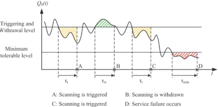
characterizing the event. A service failure during [m− 1, m] is thus defined by an excursion of the serving cell’s signal quality falling below the minimum tolerable level γmin with
minimum-duration τmin:
failm, DQ0(γmin, τmin, [m− 1, m]), (7)
τt Minimum tolerable level τmin Triggering and Withrawal level τw τt Q0(t) t A B C D
A: Scanning is triggered B: Scanning is withdrawn C: Scanning is triggered D: Service failure occurs
Fig. 2. Level crossing events experienced by a mobile user
where Q0(t) denotes the SINR received from the serving cell
at time t. Fig. 2 gives an illustration. A service failure occurs at instant ‘D’, where the serving cell’s signal quality drops below γmin for a duration τmin. Note that when τmin = 0, the
definition in (7) corresponds to an instantaneous SINR outage, which is a special case of our expression.
C. Scanning Trigger
Since handover measurement introduces overheads such as gaps in data transmission or mobile’s resource consumption, one expects to perform a handover measurement only when the signal quality of the serving cell is really bad. Since a SINR may cross and stay below or above a threshold instantaneously or only for a very short duration, the handover measurement should be triggered only if the serving cell’s signal quality drops below a certain threshold, say γt, for a
certain period, denoted by τt. It is clear that if these two
parameters are not appropriately configured, it may happen that a service failure occurs before the handover measurement initiation. In such case, the mobile has to conduct a link re-establishment procedure, which is not favorable. One can see that the handover measurement is triggered during period [m− 1, m] if the serving cell’s signal quality is worse than threshold γt during at least τt and when no service failure
occurs in this period, i.e.,
trigm, DQ0(γt, τt, [m− 1, m]) ∧ ¬ failm, (8)
where∧ and ¬ stand for logical and and logical negation, respectively. It is clear that γt should be set greater than γmin. For illustration, in Fig. 2, the handover measurement is triggered at instant ‘A’ and also at instant ‘C’, respectively.
D. Scanning Withdrawal
Similarly, the handover measurement should be withdrawn when the signal quality of the serving cell becomes good. Precisely, it should be withdrawn if the serving cell’s signal quality is higher than a threshold γw for a certain period τw.
So, the event of scanning withdrawal during period [m−1, m] is expressible as:
wdrawm, UQ0(γw, τw, [m− 1, m]). (9)
In Fig. 2, we consider that γw = γt and τw = τt. Since Q0(t) crosses over γt and stays above over a duration τt, the
1
4 3
2
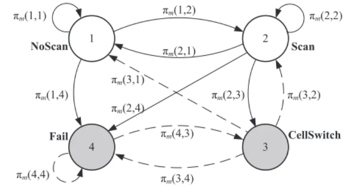
Transition involving serving cell Transition excluding serving cell πm(1,2) πm(2,1) πm(2,2) πm(1,1) πm(1,4) πm(2,3) πm(3,2) πm(4,3) πm(3,4) πm(4,4) πm(3,1) πm(2,4) CellSwitch Scan NoScan Fail
Fig. 3. State diagram of the mobile in connected-mode in the network
V. HANDOVERSTATEDIAGRAM
In consequence, a handover measurement would result in
failure if a service failure occurs, see e.g., instant ‘D’ in
Fig. 2, and success if a suitable handover target is found before its occurrence. It is particularly of primary importance to determine the probability of handover measurement failure, and also related metrics.
The mobile’s handover measurement activities during a connected-mode in a cellular network can be described by the four states capsuled in Fig. 3. States Scan and NoScan describe whether the mobile is scanning neighboring cells or not. States Fail and CellSwitch describe if the mobile is encountering a service failure or if it is being switched to another cell, respectively. For ease of analytical development, we number the four states as 1 to 4, as shown in Fig. 3. The transition probability from state i at instant m− 1 to state j at instant m, where i, j ∈ {1, 2, 3, 4}, is denoted by πm(i, j).
Denote by
πm:= (πm(1), πm(2), πm(3), πm(4))
the row vector of the state probability at instant m. Vector
π0 corresponds to the starting instant 0. In the following, we explain the details of the state diagram one by one, which is the core for all the performance evaluation.
A. State Analysis: NoScan
From state NoScan, a mobile will start a handover mea-surement and enter state Scan if the triggering condition occurs. It will fall into state Fail if the mobile encounters a service failure during the period [m− 1, m]. Otherwise, it remains in state NoScan.
Note that a mobile does not scan neighboring cells when be-ing in state NoScan. As a consequence, there is no transition from NoScan to CellSwitch, unless the network may force the mobile to connect to another cell out of the procedure. One can see that reducing scanning overhead by increasing the state probability of NoScan for example by raising the triggering threshold γt and/or prolonging the triggering duration τt will
increase the risk of service failure.
The transition probabilities πm(1, j), for j = 1, . . . , 4, are
thus expressible as:
πm(1, 2) =P(trigm),
πm(1, 3) = 0,
πm(1, 4) =P(failm),
πm(1, 1) = 1− πm(1, 2)− πm(1, 4).
(10)
B. State Analysis: Scan
In state Scan, a mobile performs handover measurement as shown in Fig. 2 while the received signal may undergo level crossings. Following Fig. 1, the transition probabilities from state Scan to the other can be written as:
πm(2, 4) =P(failm),
πm(2, 3) = (1− πm(2, 4))P(Yk≥ γreq),
πm(2, 1) = (1− πm(2, 4))P(Yk< γreq)P(wdrawm),
πm(2, 2) = 1− (πm(2, 1) + πm(2, 3) + πm(2, 4)),
(11)
where P(Yk ≥ γreq) is the probability of finding a suitable
handover target with Yk denoted by (5).
C. State Analysis: CellSwitch
In state CellSwitch, a mobile is switched to the identi-fied target cell. If the signal quality of the new serving cell is too bad or if the handover execution procedure cannot be completed, the mobile will encounter a service failure. In such case, the mobile falls into state Fail. On the other hand, given the signal quality of the new serving cell, when triggering condition holds, the mobile will then go into a Scan state and start to scan neighboring cells again; otherwise, it will go into state NoScan. Thus, the transition probabilities from state CellSwitch are expressible as:
πm(3, 2) =P(trig∗m),
πm(3, 4) =P(fail∗m),
πm(3, 1) = 1− πm(3, 2)− πm(3, 4),
(12)
where the events trig∗m and fail∗mrefer to scanning triggering
and service failure, respectively, corresponding to the signal quality received from the new serving cell, denoted by Q∗0, where the superscript ‘∗’ is used to refer to a new serving cell.
D. State Analysis: Fail
In state Fail, a mobile will re-initiate a network admission procedure or conduct link reestablishment to recover the on-going service from the interruption. The mobile scans possible neighboring cells; when a suitable cell is found, the mobile will go into state CellSwitch so as to connect to the identified cell. The signal quality of the suitable cell is required to be greater than or equal to the minimum tolerable level γmin.
Otherwise, the mobile keeps scanning to find a suitable cell, during which the service is in failure status. As a result, we have:
πm(4, 3) =P(Yk≥ γmin),
πm(4, 4) = 1− πm(4, 3).
E. State Transition Matrix
By the result of (10)-(13), the state diagram of a mobile user in the network, as illustrated in Fig. 3, can be represented by its state transition matrix expressible as:
Nm, πm(1, 1) πm(1, 2) 0 πm(1, 4) πm(2, 1) πm(2, 2) πm(2, 3) πm(2, 4) πm(3, 1) πm(3, 2) 0 πm(3, 4) 0 0 πm(4, 3) πm(4, 4) . (14) Notice that we will determine each πm(i, j) and derive their
closed-form expressions explicitly in Section VI.
To represent the time evolution of the state transitions, let
N(m), N1× · · · × Nm,
where× is the inner matrix product. It is clear that N(m)(i, j) is the transition probability from state i at instant 0 to state j at instant m.
Our objective is to derive the state diagram of the handover
measurement. Note that a mobile is connected to a current
serving cell when being in one of two states: NoScan or Scan. In contrast, the mobile enters CellSwitch or Fail. One can see that πm(1, j) and πm(2, j) depend on the signal
quality of the current serving cell, whereas πm(3, j) and
πm(4, j) do not since they occur after the connection with
the serving cell was released in case of cell switching or was interrupted in case of service failure. In the latter case, the mobile may proceed with a radio link reestablishment to resume service with a cell. From the viewpoint of mobility management, this cell is considered as a new cell even if it may be the last serving cell prior to the service interruption. However, it is important to distinguish between these two types of states for mathematical derivation. As shown in Fig. 3, CellSwitch and Fail are shadowed and their state transitions are drawn in dash-line. On the other hand, we have the state transitions from NoScan and Scan drawn in solid-line.
Note that the mobile only performs the handover measure-ment function when it is in state Scan. States CellSwitch and Fail are outcomes. From the view of a serving cell, the state diagram in Fig. 3 should be refined as Fig. 4, in which the dash-line transitions are excluded and both CellSwitch and Fail are absorbing states. Fig. 4 corresponds to the state diagram of the mobile in a handover measurement procedure. The resulting transition matrix is thus given by:
Mm, πm(1, 1) πm(1, 2) 0 πm(1, 4) πm(2, 1) πm(2, 2) πm(2, 3) πm(2, 4) 0 0 1 0 0 0 0 1 . (15) Let M(m), M1× · · · × Mm.
M(m)(i, j) is the transition probability of the handover
mea-surement from state i at instant 0 to state j at instant m. The state probability distribution πm at any instant m is
thus given by πm= π0× M(m). (16) 1 4 3 2 πm(1,2) πm(2,1) πm(2,2) πm(1,1) πm(1,4) πm(2,3) πm(3,3) πm(4,4) πm(2,4) CellSwitch Scan NoScan Fail
Fig. 4. State diagram of the mobile in handover measurement
Since the starting instant 0 corresponds to the moment when the mobile enters into connected-mode, the initial state prob-ability distribution π0 is given as
π0= (1− π0(2), π0(2), 0, 0), (17)
where
π0(2) =P(trig0) (18)
is the probability that the handover measurement is triggered at instant 0. The above formulation allows evaluating various quantities of interest, including key performance metrics of handover measurement in the next section.
F. Performance Metrics of HO Measurement
Let tc be the time interval during which the mobile has an
active connection with its serving cell, and mc =⌈tc/Tmeas⌉,
where⌈x⌉ is the smallest integer greater than or equal to x. Notice that mc is the corresponding number of measurement
periods.
As aforementioned, a handover measurement would result in two outcomes that are failure if a service failure occur during the handover measurement, and success if a suitable handover target can be found in time. The probability of
han-dover measurement failure, denoted by F, is of key concern.
With the notation developed above, we have
F = πmc(4). (19)
Similarly, the probability of handover measurement success, denoted by S, is given by:
S = πmc(3). (20)
The above expressions take into account all the involved factors including the terminal’s measurement capability k, system specified measurement time Tmeas, scan triggering and
withdrawal parameters (γt, τt) and (γw, τw), as well as HO target level γreq and service failure thresholds (γmin, τmin).
Note that the time interval tc can be treated as a
determin-istic constant or as a random variable. In the latter case, let Λ be its distribution. The above metrics can be re-written as:
F =
∫ ∞
0
and
S =
∫ ∞
0
π⌈t/Tmeas⌉(3)Λ(dt), (22) respectively. In the literature, Λ has been modeled by some known distributions such as a truncated log-logistic distri-bution. The interested reader is referred to [24] for further information.
Intuitively,F represents the probability that a service failure occurs before a suitable cell is identified, whereasS indicates the probability that the system goes into the handover decision-execution phase. It is desirable to haveF as small as possible. To do so, one may consider simply having low handover target level γreq. However, this may result in handover to cells of low
signal quality. It is thus important to assess the performance of the handover measurement by the target cell quality, which is expressible as:
Q , S × E{Yk|Yk≥ γreq}, (23)
where
E{Yk|Yk≥ γreq} = γreq+
∫ ∞
γreq
FYk(y)dy
FYk(γreq)
,
with tail distribution FYk of Yk. Note that a suitable target cell
is given by the best cell among k cells scanned and provided that its signal quality is greater than or equal to γreq.
VI. ANALYTICALCLOSED-FORMEXPRESSIONS
By the results of Section IV and V, we can derive the probabilities of findtargetm, failm, trigm, and wdrawm, cf.
(6)-(9), respectively. First, we derive findtargetm, i.e.,P(Yk≥ γ),
for any threshold γ > 0. Then, we derive P(failm) and P(trigm) built on the down-crossing events failm and trigm,
respectively. Finally, by the up-crossing event wdrawm, we
determineP(wdrawm) to complete the analytical formulation.
A. Probability of Finding a Suitable Cell
To determine the probabilityP(Yk≥ γ), one needs to define
the set of candidate cells from which k cells would be taken for the handover measurement. By today’s cellular standards [2], [21], [25], there are two cases:
• limited candidate set, and
• unlimited candidate set.
In the former, a mobile only scans neighboring cells of a pre-defined set which contains a limited number of potential candidates, say Ncell cells. The set in practice corresponds to
the neighbor cell list (NCL) as used in GSM, WCDMA, and WiMAX with Ncell = 32. In the case of unlimited candidate
set, the mobile is allowed to scan any cell in the network. However, since a network may have a very large number of cells, scanning without restriction would introduce unafford-able overheads. Therefore, new broadband cellular systems use a set of, say NCSID, cell synchronization identities (CSID), to
label cells from this finite set. Since this set of NCSID CSIDs
are shared among all the cells, two cells having the same CSID must be spatially separated far enough so as to avoid any confusion. When required to scan k cells, a mobile just picks
k out of the total NCSIDCSIDs without a pre-defined NCL and then conduct standardized cell synchronization and measure-ment. An example using this mechanism is LTE that defines 504 physical cell identifiers (PCI) which serve as CSIDs. The mobile performs the cell measurement autonomously without the need of a pre-configured cell set such as the NCL used in predecessor systems, for the generality.
We determine P(Yk ≥ γ) in both cases and complete the
details below.
1) Case of unlimited candidate set: Each neighboring cell
is scanned with equal probability ρk = k/NCSID. This set of
the scanned cells is in other words a thinning of R2 with retention probability ρk. Notice that this set of the scanned
cells, say Sk, may have more than k cells, and this efficiently
describes the real situation where the mobile may detect several cells which have the same CSID. In practice, a LTE eNodeB relies on an automatic neighbor relation table to map a reported physical cell identifier (PCI) to a unique cell global identifier (CGI). Whenever a PCI conflict is detected where two cells having the same PCI are found, the eNodeB may request the UE to perform an explicit CGI acquisition of the PCI in question, which may take long time, and updates its neighbor relation table.
In consequence, we re-write (6) as:
Yk ≡ max i∈Sk
Qi, (24)
and by definition,
P(Yk > γ) = FYk(γ), (25)
where FYk(·) is the tail distribution function of Yk. Apply
Corollary 5 in [26] for the tail distribution of Yk, we have:
Proposition 1. With the system model and notation as
de-scribed above, consider the case of unlimited candidate set with NCSID cell synchronization identities. Assume l(d) = dβ,
thenP(Yk> 0) = 1, and for γ > 0:
P(Yk > γ) = ∫ ∞ γ ∫ ∞ 0 e−C1wα−C2(w,u) π [ −1 + γ γ × cos(C1wαtan( πα 2 ) + C3(w, u) + C4(w, u) ) + cos ( C1wαtan( πα 2 ) + C3(w, u)− wu )] dwdu, (26)
where α = 2/β, ρk= k/NCSID, C1= (1− ρk)δ, and
C2(w, u) = ρkcα 1F2(−α2; 1 2, 1− α 2;− u2w2 4 ) uα , C3(w, u) = ρkcα αw 1− α 1F2(1−α2 ;32,3−α2 ;−u24w2) uα−1 , C4(w, u) = w(1− u(1 + γ)/γ),
in which 1F2 denotes the hypergeometric function, and δ = cαΓ(1− α) cos(πα/2), (27)
with Γ(·) denoting the gamma function, and cα= πλPtxαexp
(
α2σZ2/2), with σZ = σXlog 1010 .
Proof: By the discussion of (24), Yk is the best
sig-nal quality of a thinning of R2 with retention probability ρk = k/NCSID. Under assumptions that Ptx is a finite positive
constant and Zi = 10Xi/10 with Xi being Gaussian and
0 < σX < ∞, PtxZi admits a continuous density and
0 < E{(PtxZi)α} < ∞. Provided l(d) = dβ, P(Yk > γ)
is then given by Corollary 5 in [26].
2) Case of limited candidate set: Consider bB a disk-shaped
network area with radius:
RBb=√Ncell/(πλ). (28)
Under the assumption that base stations are distributed accord-ing to a Poisson point process, bB has on average Ncell base stations. Thus, by approximating the region of the Ncell
neigh-boring cells by bB, we have the tail distribution P(Yk > γ)
directly given by Theorem 3 in [26]. In particular, we can have some more tractable expression of P(Yk > γ) by considering
the following two cases: scattered networks like rural macro cellular networks where inter-site distance is large such that the network density λ is small, and dense networks like urban small cell networks where a large number of cells are deployed to support dense traffic such that λ is large.
For small λ, we can have RBb ≈ ∞, i.e., bB can be
approximated by R2. Similarly, let Sk be a thinning on bB
with retention probability:
ρk= k/Ncell (29)
such that Skhas on average k cells. The probability of finding
a target cell can be obtained according to Proposition 1. For large λ (e.g., a dense network), the approximation
RBb ≈ ∞ may be not applicable. In addition, under the
assumption that base stations are distributed according to a Poisson point process, the probability that a base station is found very close to a given user may be significant. The
unbounded path loss model (i.e., dmin = 0) may be no
longer suitable because the effect of its singularity is now non-negligible. Therefore, bounded path loss with dmin> 0 is
considered. The probability of finding a suitable cell is given by the following proposition.
Proposition 2. With system model and notation as described above, consider the case of limited candidate set with Ncell,
and large λ. Let bB be a disk-shaped network area of radius RBb=√Ncell/(πλ). Then:
(i) Yk is the best signal quality received from ˆk cells
uniformly selected from bB where ˆk = min(k, Ncell).
(ii) Assume dmin> 0, for γ≥ 0:
P(Yk > γ)≈ ∫ ∞ γ { g(u) ∫ ∞ 0 2 πwe −δwα sin(wu− γ 2γ ) × cos(wu + wu− γ 2γ − δw αtanπα 2 ) dw } du, (30)
where approximation holds under the condition that Ptxd−βmin is large, δ is given by (27), and
g(x) = ˆk· fP(x)· F ˆ k−1 P (x), for ˆk≥ 1, with FP(x) = c (K 1(x) aα − K2(x) bα − ewK 3(x) xα + ewK 4(x) xα ) , where w = 2σ2 X/β2, a = PtxR−βBb , b = Ptxd−βmin, c = Ptxα(R2b B− d 2
min)−1, and Kj, j = 1, . . . , 4, refer to the
lognormal distributions of parameters (µj, σZ) with
µ1= log a, µ3= µ1+ 2σZ2/β,
µ2= log b, µ4= µ2+ 2σZ2/β,
and fP(x) = dFP(x)/dx.
Proof: Assertion (i) follows from the above discussion
considering that the mobile station scans at most Ncell by its
measurement capacity k. Under the assumption dmin> 0, (30)
is given following Theorem 2 in [27].
In Proposition 2, Ptxd−βmin is nothing but the average signal
power received at the excluding distance dmin. The average
here is with respect to the unit mean fading Zi. The
ap-proximation condition that Ptxd−βmin is large implies that the
excluding distance should be small compared to the cell size.
B. Probability of Service Failure:P(failm)
Recall (7), where Q0(t) is the SINR received from serving
cell at time t, Q0(t) < γmin is equivalent to X(t) < ˆγmin(t)
in a logarithmic representation, where ˆ γmin(t), 10 log10 ( γmin l(d(t)) Ptx (1 + I(t)) ) , (31) by substituting (1) and (2) into (4). Note that the excursions of non-stationary process Q0(t) below threshold γmin is now
represented by the excursions of a stationary normal process
X(t) (cf. (2)) below the time-varying level ˆγmin(t). This
transformation would greatly facilitate the coming derivation. Let Tmin be the length of an excursion of X(t) below
ˆ
γmin(t). Following (7), failmis thus expressible as an excursion
of X(t) below threshold ˆγmin(t) with Tmin longer than τmin,
i.e.,
failm={X(t) stays below ˆγmin(t) during Tmin≥ τmin,
for t∈ [(m − 1)Tmeas− τmin, mTmeas]}, (32)
where the considered time window is [(m − 1)Tmeas −
τmin, mTmeas] as the failure will occur at a instant t0+ τmin
anterior to (m− 1)Tmeas if the excursion starts at t0 <
(m− 1)Tmeas− τmin.
We will use the level crossing properties of X(t) to derive the probability of event failm. Given a constant level γ, we
can have the following results.
Lemma 3( [23], p.194). Write Cγ the number of crossing of
X(t) of level γ during a unit time,
ECγ = 1 π √ λ2 λ0 exp ( −γ2 2λ0 ) , (33) with λ0= RX(0), and λ2=−RX′′(τ )|τ =0. ECγ< +∞ if and only if λ2< +∞.
In addition, let Uγ and Dγ be the number of up-crossings
and the number of down-crossings of X(t) of level γ during a unit time, respectively. One can find that [23, p.197]:
EUγ =EDγ =ECγ/2. (34)
Proposition 4. With X(t) described above, for constants γ and τ , define
V (γ, τ ), P(X(t) stays above γ during at least τ). Consider the following assumptions on RX(τ ):
(i) there exists finite λ2, and a > 1: RX(τ ) = 1−
λ2τ2
2 +O(τ
2| log |τ||−a), as τ → 0, (35)
(ii) there exists finite λ2 and finite λ4: RX(τ ) = 1− λ2 2!τ 2+λ4 4!τ 4+ o(τ4), as τ → 0, (36)
(iii) there exists a > 0:
RX(τ ) = O(τ−a), as τ → +∞, (37)
Then:
• For γ→ +∞, under conditions (35) and (37), V (γ, τ ) =EUγ· ( τ exp(−Aγτ2) + √ π Aγ Q(√2Aγτ ) ) , where Aγ = π 4 ( EUγ Q(γ/σX) )2 , and Q(x), ∫ ∞ x e−t2/2 √ 2π dt.
• For γ→ −∞, under conditions (36) and (37), V (γ, τ ) =EUγ· exp(−µτ) · (τ + 1/µ),
where µ =EUγ/Q(γ/σX).
Proof: Please see Appendix B.
Notice that under condition (37), the wide sense stationary process X(t) is mean-ergodic [28]. Thus, for all intervals [t1, t2], one can have:
P(X(t) stays above γ during at least τ, t ∈ [t1, t2]) =P(X(t) stays above γ during at least τ). The result of Proposition 4 is thus applicable for the probabil-ity of excursions with minimum required duration considering a finite time interval.
Using Proposition 4, we can obtainP(failm) for a constant ˆ
γmin. However, note that ˆγmin(t) is time varying due to I(t) and
d(t). Under the model described in Section III, interference I
can be modeled as a shot noise onR2[29]. For l(d) = dβ, its characteristic function is expressible as [26], [30]:
ϕI(w) = exp
(
− δ|w|α[1− jsign(w) tan(πα/2)]), (38)
where δ is given by (27). By the assumption that β > 2, 0 < α < 1 since α = 2/β. In consequence, one can see that ϕI(w) is absolutely integrable. By the inverse formula
[31, Thm.3], the probability density function (pdf) of I can be obtained: fI(x) = 1 π ∫ ∞ 0 e−δwαcos ( δ tan(πα 2 )w α− xw) dw. (39)
On the other hand, τmin and Tmeas are typically about a few
hundreds of milliseconds (e.g., Tmeas = 200ms under LTE
standard [22]). The interval Tmeas+τminis so short that wherein
the distance between the mobile and its serving base station can be considered constant. By the above results, we can have: Proposition 5. With the system described above, assume that
RX(τ ) satisfies conditions (35) – (37), and l(d) = dβ. Then,
P(failm| d(t) = dm) =
∫ ∞
0
V (−ˆγmin, τmin)fI(x)dx, (40)
where fI is given by (39), V is given by Proposition 4, and
ˆ γmin, 10 log10 ( γmindβm Ptx (1 + x) ) . (41)
Moreover, if d(t)≈ dmfor t∈ [(m − 1)Tmeas− τmin, mTmeas],
one can have:
P(failm)≈ P(failm| d(t) = dm), accordingly.
Proof: Under the considered assumptions, I admits
den-sity fI. So, we write:
P(failm| d(t) = dm) = ∫ ∞ 0 P(failm| I(t) = x, d(t) = dm)fI(x)dx, in which by (32), P(failm| I(t) = x, d(t) = dm)
=P(X(t) stays below ˆγmin during Tmin≥ τmin) (∗)
= P(X(t) stays above − ˆγmin during Tmin ≥ τmin),
where (∗) is by the fact that normal process X(t) is statisti-cally symmetric around its zero mean. The result thus follows using Proposition 4.
Remark 6. If one may consider users moving at very high
speeds such that d(t) changes significantly during the time interval Tmeas + τmin, P(failm) can then be computed by a
knowledge of the distribution of d(t) with a corresponding mobility model. Here we make the above approximation for simplification.
C. Probability of Scanning Trigger:P(trigm)
By the definition of the scanning trigger event trigm given in (8), we have:
P(trigm) = P(DQ0(γt, τt, [m− 1, m]) ∧ ¬ failm)
= P(DQ0(γt, τt, [m− 1, m]))
− P (DQ0(γt, τt, [m− 1, m]) ∧ failm) . (42)
Similar to the treatment on DQ0(γmin, τmin, [m− 1, m]) in
Section VI-B for computing P(failm), and the treatment on
DQ0(γt, τt, [m− 1, m]), by the result of Proposition 5, the
first term on the right-hand side of (42) is given by:
P(DQ0(γt, τt, [m− 1, m])|I(t) = x, d(t) = dm) = V (−ˆγt, τt), (43) where ˆ γt, 10 log10 (γtdβ m Ptx (1 + x) ) . (44)
For the second term on the right hand-side of (42), we have: P(DQ0(γt, τt, [m− 1, m]) ∧ failm| I(t) = x, d(t) = dm
) =P(X(t) stays below ˆγmin during Tmin≥ τmin,
and X(t) stays below ˆγt during Tt≥ τt
)
. (45) This turns out to be the probability of successive excursions of two adjacent levels. The following result is useful. Lemma 7. ( [32, (30)-(33)]) With X(t) described above, for
γ2≥ γ1, τ1≥ 0, and τ2≥ 0, let A := Aγ1, τ1∗:= γ1(γ2− γ1) A , and τ2∗= √ τ2 1 − τ1∗, for τ 2 1 ≥ τ1∗. Define
W (γ1, τ1, γ2, τ2) :=P(X(t) stays above γ1during at least τ1and X(t) stays above γ2during at least τ2).
Put W := W (γ1, τ1, γ2, τ2) for simplicity. If RX(τ ) satisfies
conditions (35) - (37), • for τ12≤ τ1∗ and τ2= 0, W =EUγ1 eAτ12 e2Aτ1∗ √ π 4A, • for τ2 1 ≤ τ1∗, and τ2> 0, W =EUγ1 eAτ2 1 e2Aτ1∗ ( τ2 eAτ2 2 + √ π 4Aerfc( √ Aτ2) ) , • for τ12> τ1∗, and τ2= 0, W = EUγ1 eAτ2 1 √ π 4A, • for τ12> τ1∗ and 0 < τ2≤ τ2∗, W =EUγ1 eAτ2 1 ( τ2∗+ √ π 4A erfc(√Aτ2∗) exp(−A(τ2∗)2) ) , • for τ2 1 > τ1∗ and τ2> τ2∗, W =EUγ1 eAτ2 1 ( τ2 eA(τ2 2−(τ2∗)2) + √ π 4A erfc(√Aτ2) e−A(τ2∗)2 ) , as γ1→ +∞.
By the above analysis, we have the following conclusion. Proposition 8. Assume that RX(τ ) satisfies conditions (35) –
(37), and l(d) = dβ. Consider that γt≥ γmin, we have:
P(trigm| d(t) = dm)
=
∫ ∞
0
(V (−ˆγt, τt)− W (−ˆγt, τt,−ˆγmin, τmin))fI(x)dx,
where fI, V , and W are given by is given by (39),
Proposi-tion 4, and Lemma 7, respectively, with ˆγminand ˆγtgiven by
(41) and (44), respectively.
Proof: Following the above assumptions, I has pdf fI as
given by (39). So, we have: P(trigm| d(t) = dm)
=
∫ ∞
0
P(trigm| I(t) = x, d(t) = dm)fI(x)dx.
Regarding (45), as X(t) is statistically symmetric around its zero mean, one can have:
P(DQ0(γt, τt, [m− 1, m]) ∧ failm| I(t) = x, d(t) = dm
) =P(X(t) stays above − ˆγmin during Tmin≥ τmin,
and X(t) stays above − ˆγt during Tt≥ τt
)
,
where noting that−ˆγt≤ −ˆγmin, considering γt ≥ γmin. This
is obtainable by Lemma 7. Using this and (43), the result follows.
D. Probability of Scanning Withdrawal:P(wdrawm)
The probability of wdrawm defined in (9) can be obtained
by the same technique used in Section VI-B. Note that
Q0(t)≥ γw is equivalent to X(t)≥ ˆγw(t) with ˆ γw(t), 10 log10 ( γw l(d(t)) Ptx (1 + I(t)) ) .
The scanning withdrawal wdrawm is then expressible as an
up-excursion of X(t) above the level ˆγw(t) for Tw≥ τw: wdrawm={X(t) stays above ˆwmin(t) during Tw≥ τw,
for t∈ [(m − 1)Tmeas− τw, mTmeas]}. So, similar to Proposition 5, we can have:
Proposition 9. With the system described above, assume that
RX(τ ) satisfies conditions (35) – (37), and l(d) = dβ. Then,
P(wdrawm| d(t) = dm) = ∫ ∞ 0 V (ˆγw, τw)fI(x)dx, where ˆ γw, 10 log10 ( γwdβm Ptx (1 + x) ) ,
and fI and V are given by (39) and Proposition 4, resp.
VII. APPLICATIONS
Using the above framework, we investigate the handover measurement in LTE and in particular the influence of key parameters on the system performance.
A. System Scenarios
1) Deployment scenarios: Parameters are summarized in
Table II following 3GPP recommendations [4], [33] for two deployment scenarios of LTE networks, including urban and rural macro-cellular networks. For each scenario, the network density λ is set corresponding to hexagonal cellular layout of 3GPP standard, resulting in λ = 2/(3√3R2) BS/m2.
The user’s mobility is characterized in terms of his or her moving direction and velocity. The user is assumed to be moving away from the serving base station at velocity v. This scenario has been considered as the most critical circumstance
TABLE II
DEPLOYMENT SCENARIOS
Parameter Assumption
Urban macro-cell
Path loss (d in km) l(d) = 128.1 + 37.6 log10d
Transmit power PBS= 43 dBm
Antenna pattern Omnidirectional
Cell radius R = 1000 m
User’s velocity v = 50 km/h
Rural macro-cell
Path loss (d in km) l(d) = 95.5 + 34.1 log10d
Transmit power PBS= 46 dBm
Antenna pattern Omnidirectional
Cell radius R = 1732 m
User’s velocity v = 130 km/h
Shadowing Standard deviation σX = 10 dB
Decorr. distance dc= 50 m
Noise Noise density =−174 dBm/Hz
UE noise figure NF= 9 dB
[33]. The velocity is assumed constant and is set according to maximum speed authorized by regulations, typically 50 km/h in cities, and 130 km/h in highways.
In lognormal shadowing, the square-exponential autocorre-lation model [34], [35] is used:
RX(τ ) = σ2Xexp ( −1 2 (vτ dc )2) ,
where dc is the decorrelation distance. This model satisfies
conditions required in Section III. Its second spectral λ2 is
given by:
λ2=−R′′X(τ )|(τ =0)= (σXv/dc)2.
2) Service requirements: The minimum allowable level γmin and minimum duration to service failure τmin are set
according to the condition of a radio link failure specified by LTE standard [4, Ch.7.6]. When the downlink radio link quality estimated over the last 200 ms period becomes worse than a threshold Qout, Layer 1 of the UE shall send an out-of-sync indication to higher layers. Upon receiving N310
consecutive out-of-sync indications from Layer 1, the UE will start timer T310. And upon the expiry of this timer,
the UE considers radio link failure to be detected. It can be consequently concluded that a radio link failure occurs if the signal quality of the serving cell is worse than γmin = Qout
during at least
τmin= 200[ms]· N310+ T310.
Following the parameters specified in [4, Ch.A.6], N310= 1
and T310= 0. This yields τmin = 200 ms. The threshold Qout
is defined in [4, Ch.7.6.1] as the level at which the downlink radio link cannot be reliably received and corresponds to 10% block error rate of Physical Downlink Control CHannel (PDCCH). Note that Qoutis as small as−10 dB [33, Ch.A.2].
Besides, various settings of γmin are evaluated, as summarized
in Table III.
The target cell’s quality is required to be higher than the minimum tolerable level γmin by a handover margin δHO such
that γreq= γmin+ δHO.
TABLE III
SERVICES ANDCONFIGURATION
Parameter Assumption
Services
Min time to failure τmin= 200 ms Min level to failure γmin=−20 to −5 dB
Handover margin δHO= 2 dB
Req. target level γreq= γmin+ δHO Continual
Measurement
Measurement period Tmeas= 200 ms
Triggering level γt= +∞
Withdrawal level γw= +∞
Triggered Measurement
Measurement period Tmeas= 200 ms
Scan margin δscan= 20 dB
Triggering level γt= γmin+ δscan Withdrawal level γw= γmin+ δscan
Min time to trigger τt= 200 ms
Min time to withdraw τw= 1024 ms
3) System configuration: The LTE standard assumes that
UEs perform the handover measurement autonomously using 504 physical cell identifiers (PCIs) without neighbor cell list (NCL), the probability of finding a suitable handover target P(findtargetm(k)) is thus given by Proposition 1 with retention
probability ρk= k/NCSID, where NCSID= 504.
The conventional configuration of LTE standard specifies that a UE measures neighboring cells as soon as it enters connected-mode. This configuration is commonly referred to as continual handover measurement. This setting corresponds to triggering level and withdrawal level set to infinity, i.e.,
γt = +∞, and γw = +∞, so that π0(2) = 1, and P{wdrawm} = 0 according to (9). On the other hand,
P(trigm) = 1− P(failm)
according to (42), for all m. This implies πm(1, 1) = 0
fol-lowing (10). Note that in this case of continual measurement, the transition matrix reduces to:
Mm= 0 πm(1, 2) 0 πm(1, 4) 0 πm(2, 2) πm(2, 3) πm(2, 4) 0 0 1 0 0 0 0 1 . Beside the above conventional configuration, we also con-sider triggered handover measurement in which γtand γware
set to the same finite threshold given by
γt= γw= γmin+ δscan,
where δscan is the scan margin. This setting helps examining
the influence of the system configurations, and also showing the capability of the developed model. The parameters are summarized in Table III.
B. Validation
A computer simulation was built with the above urban macro-cell scenario in order to check the accuracy of the models developed in Section VI. The interference field was generated according to a Poisson point process with intensity
λ in a 100 km2 region, and the serving base station is located
10−4 10−2 100 102 104 0 0.2 0.4 0.6 0.8 1 γ P(Y k > γ ) Simulation Analytical k = 504 k = 128 k = 32 k = 8
(a) Tail distribution of Yk
0 200 400 600 800 1000 0 0.2 0.4 0.6 0.8 1 m P(fail m ) Simulation Analytical γmin = −20 dB γmin = −10 dB
(b) Level crossing analysis Fig. 5. Validation of analytical model. Network scenario is urban macrocell.
100 101 102 10−7 10−6 10−5 10−4 10−3 10−2 measurement capacity, k F γ min = −20 γ min = −15 γ min = −10 γ min = −5
(a) Measurement failure probabilityF
100 101 102 22 24 26 28 30 32 34 measurement capacity, k Q in dB γmin = −20 γmin = −15 γmin = −10 γmin = −5
(b) Target cell qualityQ Fig. 6. Continual measurement in rural macrocell (Scenario 1).
generated as the output of an infinite impulse response filter with input Gaussian noise of standard deviation σX.
First, Fig. 5(a) verifies our analytical model against com-puter simulation for the tail distribution of the best signal quality ¯FYk of Proposition 1, which corresponds to common
LTE setting described above. The agreement of the results by the proposed analytical expressions and simulations illustrates the accuracy of modeling the best signal quality Yk defined in
(6) by the maximum of SINRs received from the thinning Sk
proposed in (24).
Fig. 5(b) checks the analytical framework based on level crossing analysis which was used to derive the probabilities of service failure, scanning triggering, and scanning withdrawal. Results show that both the analytical model and the simulation provide agreed results of the probability of service failure P(failm) in both settings.
C. Results
With the accuracy provided by the proposed analytical framework, we investigate numerical results of the defined performance metrics for the following scenarios:
• Scenario 1: Rural with continual measurement
• Scenario 2: Rural with triggered measurement
• Scenario 3: Urban with continual measurement
• Scenario 4: Urban with triggered measurement
1) Continual measurement in rural macrocell: Fig. 6 evalu-ates the performance of handover measurement in this scenario for different service requirements and measurement capacity. It shows that the handover measurement failure probability
F and the expected quality of target cell Q are enhanced by
increased measurement capacity k. This is by the fact that higher k improves the distribution of the maximum SINR, cf. Fig. 5(a) or see [26], [27] for analytical implication, resulting in higher probability that a UE will find a suitable target cell. Fig. 6 also indicates the dependence of F and Q on the
100 101 102 10−3 10−2 10−1 measurement capacity, k F γ min = −20 γ min = −15 γ min = −10 γ min = −5
(a) Measurement failure probabilityF
100 101 102 22 24 26 28 30 32 34 measurement capacity, k Q in dB γ min = −20 γ min = −15 γ min = −10 γ min = −5
(b) Target cell qualityQ Fig. 7. Triggered measurement in rural macrocell (Scenario 2).
20 25 30 35 10−4 10−3 10−2 10−1 Scan margin (dB), δ scan F γ min = −20 γ min = −15 γ min = −10 γ min = −5 (a) 20 25 30 35 0.95 0.96 0.97 0.98 0.99 1 Scan margin (dB), δ scan S γ min = −20 γ min = −15 γ min = −10 γ min = −5 (b) Fig. 8. Influence of scan margin δscan. Rural macrocell with measurement capacity k = 8.
service requirement γmin. For more constrained services (i.e.,
higher γmin), the probability of service failure is higher,
leading to higher probability of handover measurement failure as seen in Fig. 6(a). On the other hand, from Fig. 6(b), the quality of target cell Q is proportionally enhanced with higher required level of target cell quality γreq, which is set to γmin+ δHO with δHO= 2 dB in this scenario.
Note that the increasing rate of Q with high γreq(= γmin+ δHO) is smaller than that of low γreq, see Fig. 6(b). Besides, as
shown in Fig. 6(a),F is below 10−2and flats out around k = 8 for all cases. Hence, for the continual handover measurement in a rural macrocell environment, supporting low measurement capacity could be enough for reliable handover measurement. This setting is also good for reducing mobile’s power con-sumption. One can confirm that k = 8 recommended by 3GPP standard is indeed efficient. On the other hand, setting a relatively high γreqcould arrive a higher expected target cell
qualityQ. However, the tradeoff is that it may lead to higher
failure probabilityF.
2) Triggered measurement in rural macrocell: The contin-ual measurement as seen above provides good performance in terms of low failure probability. However, it consumes ter-minal’s battery by continuously processing cell measurement when in connected mode. An option for reducing this is to use triggered measurement.
For the triggered measurement, Fig. 7 shows F and Q
with respect to the measurement capacity while the service requirements are similar to those in continual measurement. Compared to the former case (see Fig. 6), the failure prob-ability is clearly higher, however the target cell quality only has minor degradation.
Note that indeed the continual measurement is a triggered measurement with δscan = +∞. Fig. 8 shows how triggered
measurement could degrade the performance of handover mea-surement in terms of the scan margin δscan. The higher is δscan,
the more room the mobile can have to find a target cell before a service failure, resulting in better handover measurement
0 200 400 600 800 1000 0 0.1 0.2 0.3 0.4 0.5 0.6 0.7 0.8 0.9 1 measurement instant, m P( fail m ) rural urban γ min = −20 γ min = −5
(a) Service failure probability
−50 −40 −30 −20 −100 0 10 20 30 40 50 0.1 0.2 0.3 0.4 0.5 0.6 0.7 0.8 0.9 1 γ (dB) FY ( γ ) rural urban k=128 k=8
(b) Distribution of maximum SINR Fig. 9. Urban macrocell versus rural macrocell.
100 101 102 10−6 10−5 10−4 10−3 10−2 10−1 100 measurement capacity, k F γ min = −20 γ min = −15 γ min = −10 γ min = −5 (a) 100 101 102 22 24 26 28 30 32 34 36 38 measurement capacity, k Q in dB γ min = −20 γ min = −15 γ min = −10 γ min = −5 (b) Fig. 10. Continual measurement in urban macrocell (Scenario 3)
performance in terms of lower failure probability and higher success probability. Besides, comparing Fig. 6(a) at k = 8 and Fig. 8(a) at δscan= 20, we can see thatF increases by a factor
of more than 102when moving from continual measurement to
triggered measurement. This explains significant degradation of F observed in Fig. 7(a) compared to Fig. 6(a).
On the other hand, Fig. 8(b) shows that the success probabil-ityS is already near to 1. The influence on S when changing
δscan from +∞ (i.e. continual measurement) to 20 dB is less
significant. This results in relatively small degradation of Q. The counterpart is that the mobile performs handover mea-surement more frequently when setting higher scan margin
δscan, leading to more power consumption. One question of interests thus is the optimal setting of δscan to get a good
tradeoff between the handover measurement performance and the power consumption. As far as the information on the power consumption due to handover measurement is unavailable, it can be efficient to set δscan to the minimum value for which
the failure probability is below a target level, e.g., 10−2.
3) Continual measurement in urban macrocell: We now assess the influence of the network environment and user’s mobility on the handover measurement by considering urban macrocell network in which the user’s velocity is lower than that in the rural macrocell case, cf. Table II.
As seen from the analytical results, the failure probabilityF depends on various parameters including the distribution of the maximum SINR, and the service failure probability. The latter in turn depends on the user’s mobility. Fig. 9(a) shows that the service failure probability is higher in rural case than in urban. However, as the distribution of the maximum SINR in the urban macrocell is worse, cf. Fig. 9(b), it results in higher probabilityF compared to that in the rural macrocell case, cf. Fig. 10(a) and Fig. 6(a). For the same target level ofF at 10−2 as above, measurement capacity k = 8 could be only sufficient for robust services (i.e., low γmin), see Fig. 10(a). To support
more constrained services in urban macrocell environment, the mobile terminal should be able to measure as many as 100 cells per measurement period of 200 millisecond.