HAL Id: hal-01349395
https://hal-enac.archives-ouvertes.fr/hal-01349395
Submitted on 27 Jul 2016HAL is a multi-disciplinary open access archive for the deposit and dissemination of sci-entific research documents, whether they are pub-lished or not. The documents may come from teaching and research institutions in France or abroad, or from public or private research centers.
L’archive ouverte pluridisciplinaire HAL, est destinée au dépôt et à la diffusion de documents scientifiques de niveau recherche, publiés ou non, émanant des établissements d’enseignement et de recherche français ou étrangers, des laboratoires publics ou privés.
Public Domain
Optimization of 3D Cooling Channels in Injection
Molding using DRBEM and Model Reduction
Nicolas Pirc, Fabrice Schmidt, Marcel Mongeau, Florian Bugarin, Francisco
Chinesta
To cite this version:
Nicolas Pirc, Fabrice Schmidt, Marcel Mongeau, Florian Bugarin, Francisco Chinesta. Optimization of 3D Cooling Channels in Injection Molding using DRBEM and Model Reduction. International Journal of Material Forming, Springer Verlag, 2009, 2 (1), pp.271-274. �10.1007/s12289-009-0598-2�. �hal-01349395�
____________________
* Corresponding author: [email protected], 00 33 5 63 49 30 89
OPTIMIZATION OF 3D COOLING COOLING CHANNELS IN INJECTION
MOLDING USING DRBEM AND MODEL REDUCTION
N. PIRC
1, F. SCHMIDT
1, M. MONGEAU
2, F. BUGARIN
1and F. CHINESTA
31
Université de Toulouse, Institut Clément ADER, Mines Albi, CROMeP, 81013 Albi, France.
2Université de Toulouse, Université Paul Sabatier, Institut de Mathématiques, 31062 Toulouse
cedex 9, France.
3
Ecole Centrale de Nantes, Pôle matériaux et procédé de fabrication, 1 rue de la noé, BP 92101,
44321 Nantes cedex 3, France.
ABSTRACT: Today, around 30% of manufactured plastic goods rely on injection moulding. The cooling time can
represent more than 70% of the injection cycle. In this process, heat transfer during the cooling step has a great influence both on the quality of the final parts that are produced, and on the moulding cycle time. In the numerical solution of three-dimensional boundary value problems, the matrix size can be so large that it is beyond a computer capacity to solve it. To overcome this difficulty, we develop an iterative dual reciprocity boundary element method (DRBEM) to solve Poisson’s equation without the need of assembling a matrix. This yields a reduction of the computational space dimension from 3D to 2D, avoiding full 3D remeshing. Only the surface of the cooling channels needs to be remeshed at each evaluation required by the optimisation algorithm. For more efficiency, DRBEM computing results are extracted stored and exploited in order to construct a model with very few degrees of freedom. This approach is based on a model reduction technique known as proper orthogonal (POD) or Karhunen-Loève decompositions. We introduce in this paper a practical methodology to optimise both the position and the shape of the cooling channels in 3D injection moulding processes. First, we propose an implementation of the model reduction in the 3D transient BEM solver. This reduction permits to reduce considerably the computing time required by each direct computation. Secondly, we present an optimisation methodology applied to different injection cooling problems. For example, we can minimize the maximal temperature on the cavity surface subject to a temperature uniformity constraint. Thirdly, we compare our results obtained by our approach with experimental results to show that our optimisation methodology is viable.
KEYWORDS: BEM, optimisation, model reduction, injection moulding, SQP.
1 INTRODUCTION
Today, around 30 % of manufactured plastic goods rely on injection moulding, which is based on the injection of a fluid plastic material into a closed mould. The cooling time can represent more than 70 % of the injection cycle. Moreover, in order to avoid defects in the manufactured plastic parts, the temperature in the mould must be homogeneous. Thus, the design and the position of the cooling channels are crucial elements in the design of the mould. In order to decide the position and the shape of the cooling channels in the mould, designers commonly rely on experience and trial trial-and-error method. This manual design process becomes inadequate and unpractical for complex problems. As a consequence, designers need a more powerful tool integrating the cooling analysis, its numerical simulation, and even optimisation algorithms into the design process. We propose in this paper a practical methodology to
optimise both the position and the shape of the cooling channels in 3D injection moulding processes.
For the evaluation of the temperature, required both by the objective and the constraint functions, we must solve 3D heat-transfer problems via numerical simulation. Several numerical methods such as Finite Element Method (FEM) [1] [2] or Boundary Element Method (BEM) [3][4] can be used for solving the heat-transfer problem. Mathey [5] adopted the Dual Reciprocity Boundary Element Method (DRBEM), to calculate the transient temperature distributions during the cooling process, and to used BEM to solve the heat-transfer problems with a Sequential Quadratic Programming (SQP) [6] algorithm to improve mould injection cooling. She minimizes an objective function that is the weighted sum of two criteria. Her first criterion is the average temperature at the plastic-part surface. Her second criterion is the sum of the temperature variations with
respect to the average temperature. However, her approach is restricted to 2D.
Our contribution is threefold. First, we address 3D mould geometries with a BEM approach reducing the dimension of the computation space from 3D to 2D, avoiding full 3D remeshing: only the surface of the cooling channels needs to be re-meshed at each evaluation required by the optimisation algorithm. Secondly, we propose a general optimisation models that attempts at minimizing the desired overall low temperature of the plastic-part surface subject to constraints imposing homogeneity of the temperature. Thirdly, we use the reduction model [7] to reduce the CPU time of the optimisation procedure, and we demonstrate that our optimisation methodology is viable with encouraging preliminary results on a semi-industrial plastic part.
2 3D HEAT TRANSFER PROBLEM
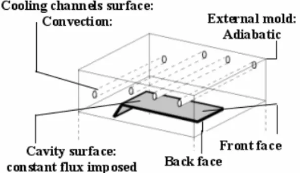
This section describes the heat-transfer problem that must be solved at every temperature evaluation required by the optimisation algorithm.To solve the heat transfer problem, the following boundary conditions must be satisfied :
Figure 1: Boundary conditions applied on the mould
3 2 1 ) ( ) ( ! " # = $ $ # ! " # = $ $ # ! " = $ $ # a a C C T T h n T k T T h n T k q n T k (1)
where !1, !2, and !3 are the mould cavity surface, the
cooling channel surface, and the mould exterior surface, respectively. The value of the instantaneous heat flux q from the polymer part to the mould can be calculated by performing a transient-part analysis using finite difference method. Here, hc represents the heat transfer
coefficient between the mould and the coolant, and ha
represents the heat transfer coefficient between the mould and the temperature channels Tc. ha represents the
heat transfer coefficient between the mould and the ambient air at a temperature Ta.
Unsteady heat conduction problems reduce to the following Poisson equation:
) t , M ( T a 1 ) t , M ( T , M"& % = & ' (2)
where t denotes time; M is the vector coordinates of a current point; a is the diffusivity, and the dot stands for the temporal derivative Eq (2) is supplemented with an initial condition T(M,t=0) and linear boundary conditions. The temperature is approximated within the entire domain ", including the boundary ! using a global interpolation formula:
(
+ = )iB j j j M t f t M T 1 ) ( ) ( ) , ( ! (3)where fj are known functions in space, #j are unknown
time-dependent functions, and I and B are respectively the number of internal nodes and collocation points located on the boundary.
Following the Dual Reciprocity Method procedure, the right-hand side of Eq (2) is approximated by Eq (3). The result is multiplied by the Green solution T*. We integrated by parts twice. We finally obtain the DRBEM integral equation :
(
*
*
*
*
++ , -.. / 0 ! # ! + + ! # ! = ! ! ! ! d T q d q T T C Td q d qT T C k k ik i k i i * ˆ * ˆ ˆ * * ! (4)Where C equal to 1 inside the domain ", and to 0.5 on its boundary $.
3 THE REDUCTION MODEL
We assume that the evolution of a certain vector field is known T(x,y,z,t). The main idea of the Karhunen-Loève (KL) decomposition is know obtain the most typical or characteristic structure %!(x,y,z,t) among these Tp(x,y,z,t).
This is equivalent to obtain a function %! maximizing #
defined by :
[
]
(
)
(
( (
= = = = = = = i N i i P p p N i i i P i P x x T x 1 2 1 2 1 ) ( ) ( ) ( " " ! (5)Using a vector notation, Eq (5) takes following matrix form : !" " " " " ! " "ˆTk = ˆT ;'ˆT 1k = (6) Where the eigenvectors do not depend on time. Let us define the following matrix Q containing the discrete field history : + + + + + , -. . . . . / 0 =
T
T
T
T
T
T
T
T
T
P N N N P P Q 2 3 4 3 3 2 2 2 1 2 2 2 1 2 1 2 1 1 2 (7)Now, we can try to use n<N eigenvectors for approximating the solution of a problem slightly
different from the one that was used to define
"
k(
x
)
5
"
k. For this purpose, we need to define the following matrix B :++ + + + , -.. . . . / 0 = ) ( ) ( ) ( ) ( ) ( ) ( ) ( ) ( ) ( 2 1 2 2 2 2 1 1 1 2 1 1 N n N N n n x x x x x x x x x B " " " " " " " " " 2 3 4 3 3 2 2 (8)
4 OVERALL OPTIMIZATION
METHODOLOGY
We first present in this section how we formulate our problem under a mathematical programming form. In the sequel, x will denote the vector of optimisation variables (position and shape parameters for the cooling channels). Since the output of the heat-transfer problem is a function of x, we shall make explicit the dependence of the temperature measurements upon the position and shape parameters
x
:
{
T
i( )
x
}
i"S.Most practical optimisation problems involve several (often contradictory) objective functions. The simplest way to proceed in such a multi-criterion context is to consider as objective function a weighted sum of the various criteria. This involves choosing appropriate weighting parameter values. An obvious alternative is to use one criterion as objective function while requiring, in the constraints, maximal threshold levels for the remaining criteria. We choose here the latter approach because we do know a threshold level value for the maximal temperature variation under which any variation is equally acceptable. More precisely, we formulate our problem under the form:
0 0 subject to ) ( min g(x) f(T(x)) x T x 6 6 (9) where f is a real-valued function used to stipulate the uniformity-temperature constraint, and g(x) is a general vector-valued non-linear function. The complete methodology to couple the thermal solver and the optimisation algorithm procedure is present in [6] The general constraints g(x) & 0 represent any geometry-related or other industrial constraints, such as:
• upper/lower-bound constraints on the xi's,
• keeping the cooling channels within the mould, • Technically-forbidden zones where we cannot
position the cooling channels (for instance due to the presence of ejectors),
• constraints stipulating a minimal distance between every pair of cooling channels to avoid inter-channels collision.
5 APPLICATION
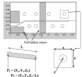
In this section, we report computational experiments on a 3D plastic part whose features are displayed on Figure 2 (unit in mm). It is a semi-industrial injection mould design for the European project: Eurotooling 21.
Figure 2 : Plastic part dimension
The history matrix, corresponding to the first injection cycle time, is computed using steady DRBEM code. The Temperature in a mould, for the next injection cycle time, is computed using the reduction model method. We use here the l! (max) norm for the objective
function: S i i x T x T " 7:=max ( ) ) ( (10)
Where S is the set of the temperature measurement locations. We optimise the cooling channel locations on our 3D model. For illustration purposes, we consider here 8 cooling channels. We choose for the optimisation routine, the Matlab8 optimisation toolbox SQP subroutine fmincon [6].
Figure 3 : Initial and optimised position of the cooling
channels.
The geometrical optimisation parameters are here the coordinates of the end points, P1 and P2 of each cooling
channel (Figure 3). Since P2 can be expressed in terms of
the other coordinates and since the channel length (L) is constant, the optimisation parameters for locating the ith cooling channel are completely determined by P1 = Xi, Yi, Zi, i = 1 . . . 8. For our application Zi is fixed and
therefore our problem involves 16 optimisation variables. We use as starting point, a heuristic solution provided by an experienced engineer. On average, one
objective function evaluation requires 14 min of CPU time. Since, we compute gradients using finite difference approximation, one optimisation iteration involves 4H of CPU time (Figure 4).
Figure 4 : Optimised position of the cooling channels.
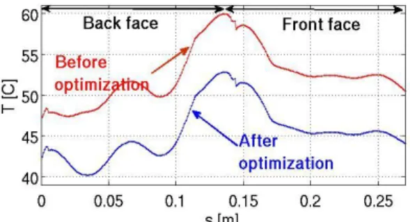
Figure 5 : Temperature profile at the surface of the
mould cavity before and after optimisation.
One of the advantages of our optimisation approach is that the user-provided initial channel geometry is not required to satisfy all constraints. Moreover, the optimised geometry is guaranteed to satisfy all constraints. We observe on Figure 5 both temperature variance and temperature average decrease significantly.
Figure 6 : Temperature history of the first 40 cycles.
On Figure 6, Curves (a) and (b) give respectively the maximum of the temperature in the cavity before and after optimisation. Curve (c) represents the average temperature at the cavity surface after optimisation.
The reduction model permit to reduce the CPU of the optimisation from 100H to DRBEM alone 7,4H for DRBEM + RM.
CONCLUSION AND PROSPECTS
We introduced a methodology based on the use of DRBEM to solve the heat transfer equation during the cooling step of the moulding process, for a 3D problem. Our preliminary tests on a semi-industrial plastic part showed that our approach is viable for optimising the design of cooling channels for injection moulding. Our modelling and optimisation methodology can easily take into account a large range of industrial constraints. Various optimisation criteria can be provided by the user (either directly as a cost function or within constraints). We presently work on more complex 3D moulds with more general parameterisations of the cooling channels. This optimisation methodology reduction model by a factor 30. We used gradient optimisation algorithm, so it will be important to study the influence of initials conditions.
ACKNOWLEDGEMENT
This study was conducted within the framework of the European project EUROTOOLING 21 (IP 505901-5, www.eurotoolin21.com).
REFERENCES
[1] Silva L., In Parallel computation for solving efficiently, 3D viscoelastic fluid flow problems, International, Polymer Processing XX, 265-273, 2005.
[2] Park S.J. Optimization method for steady conduction in special geometry using a BEM, International Journal for Numerical Methods in Engineering 43, 1109-1126, 1998.
[3] Brebbia C., Domiguez J., Boundary elements: An introductory course, WIT Press/Computational Mechanics Publication, 1992.
[4] Bialecki A, Jurgas P, Kuhn G, Dual reciprocity BEM without matrix inversion for transient heat conduction, Engineering Analysis with Boundary Element, 26, 227-236, 2002
[5] Mathey E., Automatic optimisation of the cooling of injection mold based on the boundary element method, Numiform 712, 222-227, 2004.
[6] The MathWorks, User’s Guide, Optimization Toolbox For Use With Matlab, Version 2, 2002. [7] Ammar A, Ryckelynck D, Chinesta F, Keunings R,
Journal of Non-Newtonian Fluid Mechanics, Elsevier ,134, 136-147, 2006.
[8] Jui-Ming L., Multi-objective optimization scheme for quality control in injection molding, Journal of Injection Molding Technology 6 (4), 2002.