Music feature maps with convolutional neural networks for music genre classification

(1)

OATAO is an open access repository that collects the work of Toulouse

researchers and makes it freely available over the web where possible

Any correspondence concerning this service should be sent

to the repository administrator:

tech-oatao@listes-diff.inp-toulouse.fr

This is a publisher’s version published in:

https://oatao.univ-toulouse.fr/

2 2107

To cite this version:

Sènac, Christine

and Pellegrini, Thomas

and Mouret, Florian

and

Pinquier, Julien

Music feature maps with convolutional neural networks for

music genre classification.

(2017) In: International Workshop on Content-Based

Multimedia Indexing (CBMI), 19 June 2017 - 21 June 2017 (Florence, Italy).

Official URL:

https://doi.org/10.1145/3095713.3095733

(2)

Music Genre Classification

Christine Senac

IRIT, Université de Toulouse 118, route de Narbonne Toulouse, France 31062 christine.senac@irit.fr

Thomas Pellegrini

IRIT, Université de Toulouse 118, route de Narbonne Toulouse, France 31062 thomas.pellegrini@irit.fr

Florian Mouret

IRIT, Université de Toulouse 118, route de Narbonne Toulouse, France 31062 florian.mouret@gmail.com

Julien Pinquier

IRIT, Université de Toulouse 118, route de Narbonne Toulouse, France 31062 julien.pinquier@irit.fr

ABSTRACT

Nowadays, deep learning is more and more used for Music Genre Classification: particularly Convolutional Neural Networks (CNN) taking as entry a spectrogram considered as an image on which are sought different types of structure.

But, facing the criticism relating to the difficulty in understand-ing the underlyunderstand-ing relationships that neural networks learn in presence of a spectrogram, we propose to use, as entries of a CNN, a small set of eight music features chosen along three main music dimensions: dynamics, timbre and tonality. With CNNs trained in such a way that filter dimensions are interpretable in time and frequency, results show that only eight music features are more efficient than 513 frequency bins of a spectrogram and that late score fusion between systems based on both feature types reaches 91% accuracy on the GTZAN database.

CCS CONCEPTS

• Computing methodologies → Neural networks;

KEYWORDS

convolutional neural networks, music features, music classification ACM Reference format:

Christine Senac, Thomas Pellegrini, Florian Mouret, and Julien Pinquier. 2017. Music Feature Maps with Convolutional Neural Networks for Music Genre Classification. In Proceedings of CBMI, Florence, Italy, June 19-21, 2017, 5 pages.

https://doi.org/10.1145/3095713.3095733

Permission to make digital or hard copies of all or part of this work for personal or classroom use is granted without fee provided that copies are not made or distributed for profit or commercial advantage and that copies bear this notice and the full citation on the first page. Copyrights for components of this work owned by others than ACM must be honored. Abstracting with credit is permitted. To copy otherwise, or republish, to post on servers or to redistribute to lists, requires prior specific permission and/or a fee. Request permissions from permissions@acm.org.

1 INTRODUCTION

Firstly introduced by Tzanetakis and Cook [21] in 2002 as a pattern recognition task, Music Genre Classification (MGC) remains an active research topic in the domain of Music Information Retrieval (MIR), perhaps because it is one of the most common ways to manage digital music databases.

In most systems, MGC consists of extracting a set of features from the raw audio signal, optionally performing feature selection, and making a classification based on machine learning methods. Several works have been based on the extraction of discriminating audio features categorized as frame-level, segment-level or song level features. Frame-level features, such as Spectral Centroid, Spectral Rolloff, Octave-based Spectral Contrast, Mel Frequency Cepstral Coefficients, describe the local spectral characteristics of audio signal and are extracted from short time windows (or frames) during which the signal is assumed to be stationary. Segment-level features are obtained from statistical measures of a segment composed of several frames. Such a segment is long enough to capture the sound texture. Song-level features, such as tempo, rhythmic information, melody, pitch(es) distribution(s), give meanings to music tracks in human-recognizable terms.

The recent papers show that spectrograms obtained from audio signal have been successfully applied to MGC [2], [22]. As texture is the main visual content found in spectrograms, different types of texture have been used such as Local Binary Patterns [3], Gabor Filters [22], Weber Local Descriptor [15], etc. The classification task generally relies on supervised learning approaches such as K-Nearest Neighbor, Linear Discriminant Analysis, Adaboost, and Support Vector Machine (SVM), which have been widely used. Some works demonstrated the interest of combining acoustic and multi-level visual features reflecting the spectrogram textures and their temporal variations. This is the case for Nanni & al. [15] and for Wu & al. [22], whose approach won the Music Information Retrieval Evaluation eXchange (MIREX1) MGC contests from 2011 to 2013. But beside these approaches, deep learning is more and more used by the MIR community. This success can be explained by two reasons: the first one is that it avoids the more or less difficult extraction of carefully engineered audio features, the second one is

(3)

CBMI, June 19-21, 2017, Florence, Italy C.Senac et al.

that the deep learning hierarchical topology is beneficial for musical analysis because on one hand music is hierarchic in frequency and time and on the other hand relationships between musical events in the time domain which are important for human music perception can be analyzed by Convolutional Neural Networks (CNN). The most popular method is to use a spectrogram as an input to a CNN and to apply convolving filter kernels that extract patterns in 2D.

However, as pointed out by J.Pons, T.Lidy and X.Serra [16], "a common criticism of deep learning relates to the difficulty in un-derstanding the underlying relationships that the neural networks are learning, thus behaving like a black-box". It is why they experi-mented and showed, by playing with filter shapes, that musically motivated CNN may be beneficial. In the MIREX 2016 campaign, one of these authors showed that combining a CNN capturing tem-poral information and another one capturing timbral relations in the frequency domain is a promising approach for MGC [12].

In a previous work [13], we saw the interest of using specific mu-sic features such as timbre, rhythm, tonality and dynamics related features. But in the same time, we were limited by the classification methods, SVMs with Gaussian kernels given the best accuracy (82%) on the GTZAN database [21].

So, motivated by the interest of CNNs in the MGC task, we de-cided to use some musical features, chosen along dynamics, timbre and tonality dimensions, as input of a CNN. To this end, we relied on the topology of the CNNs used by Zhang & al. [23] and whose results (87.4%), with spectrograms as entries, surpass those of the state of the art on the GTZAN database. To make a fair comparison with their results, we used the same network topology for which we have adapted the convolutional filter sizes for our music fea-tures. Results show that only eight music features outperform the spectrogram and that a late fusion of the two networks gives better results.

2 FEATURES

In this section, we describe the different features we used and their analysis window. This window has to be small enough so that the magnitude of the frequency spectrum is relatively stable and the signal for that length of time can be considered stationary.

A window of 46.44 ms length (1024 points at 22050 Hz) seems to be the most relevant in different music studies [1].

2.1 Short-Time Fourier Transform magnitude

spectrum features

For the baseline system (same one as described in [23]), we cal-culated FFT on 46.44 ms analysis Hamming windows with a 50% overlapping and we discarded phases. The output from each frame is a 513 dimensional vector.

2.2 Music features

We chose eight music features along three main music dimensions: dynamics, timbre and tonality. This set of features (previously used in [13]) was found to give the best results for our experiments.

Except for the high level Key Clarity feature, for which we used a 6 second window with a 50% overlapping, all the other features are low frame level and were extracted with a window of 46.44 ms length and a 50% overlapping. In order to temporally synchronize

all parameters, the value of the Key Clarity obtained over a period of 6 seconds is duplicated for all the segments of 46.4 ms that make up this period.

All these features were extracted with MirToolbox [10]. 2.2.1 Dynamics feature. We used signal classical Short-term energy which is an important feature for music genre classification. Thus, Metal and Classical music are highly related with this feature. 2.2.2 Timbre features. The Zero-crossing rate (ZCR), widely used in MIR, is the rate of sign changes of a signal. In music, a high ZCR corresponds to a percussive or noisy track.

In order to estimate the amount of high frequency in a signal, we can computeBrightness [11] by fixing the cut off frequency (in our case 15 kHz) and we are looking for the amount of energy above this frequency.

The spectral distribution can be described by statistical moments: we used Spectral Flatness and Shannon Spectral Entropy. Spectral Flatness [7] indicates if the spectrum is smooth or spiky: it is the ratio between the geometric mean and the arithmetic mean of the power spectrum of the signal. The Spectral Shannon En-tropy [18] can be viewed as the amount of information contained in the spectrum and if there are predominant peaks or not.

Spectral Roughness, or sensory dissonance, appears when two frequencies are very close but not exactly the same. In our case, we compute the peaks of the spectrum, and take the average of all the dissonances between all possible pairs of peaks [17].

2.2.3 Tonality features. The Key Clarity can be useful to know if a song is tonal or atonal [10]. The key clarity is the key strength associated with the best key(s) (i.e. the peak ordinate(s)). The key strength is a score computed using the chromagram. The chroma-gram, also called Harmonic Pitch Class Profile, shows the distribu-tion of energy along the pitches or pitch classes. For example, Hip Hop has generally a low Key Clarity, whereas country and blues tend to have high values.

The Harmonic Change Detection function is the flux of the tonal centroid [8], which is calculated using chromagram, and rep-resents the chords (groups of notes) played [10].

2.3 Aggregated features

Several authors have shown improvements by aggregating features over time [21], [1]. As in [23], we aggregated the features over 3 seconds with an overlap of 1.5 second. That led to a 128 × 513 spectrogram and a 128 × 8 map of music features for each 3 second clip.

3 NETWORKS

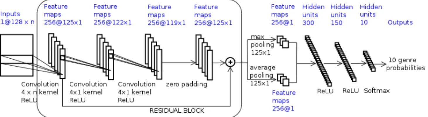
As shown in figure 1 the two networks we used are constructed on the same scheme: a residual block [9] as feature extractor and a fully connected classifier. The input of the baseline net_STFT is a Short Time Fourier Transform spectrogram (128 × 513 features) while for net_MUSIC, it is composed of the music feature map (128 × 8 music features).

Although having different intervals of variation, the music fea-tures are not standardized. Moreover, the order in which they are concatenated to form a map is not important because of the 4 × n

(4)

Figure 1: The networks topology: n corresponds to 513 frequency bins for net_STFT and to 8 music features for net_MUSIC. size filters which cause the first layer to achieve a linear

combina-tion of all of these features. These first convolucombina-tion filters with a very small time dimension of 4 (0.1 s) and with the largest feature dimension permit to model features relevant for the task, while the second and third convolution filters setting the feature size to 1 permit to find temporal dependencies.

Except for the last layer where the softmax function is applied, Rectified Linear Units (ReLUs) [14], [6] are used as the activation function in all convolutional and dense layers. ReLUs permit a good convergence even with sparse features in the hidden layers [6] and overcome the problem of vanishing gradients [5]. A single shortcut connexion (residual block) between the first and third layers permits to avoid over fitting since the training data are limited. Global temporal max- and average-pooling are used after the residual block.

The last three layers are dense with 300, 150 and 10 hidden units respectively and are used as a classifier: the outputs of the last one correspond to the 10 genre probabilities.

Each network is trained over 40 epochs and is adapted in each epoch with a mini-batch-size of 20 instances. The loss function is categorical cross-entropy, the dropout rate is 0.2 and zero padding is used before the element-wise adding operation. The hop of the convolutional kernels is one. We implemented these networks in Python with Theano [20] as a back-end. We used Theano’s GPU capabilities on an NVIDIA Tesla K40.

4 EXPERIMENTS AND RESULTS

4.1 Dataset

For our experiments, we used the GTZAN dataset [21] which, al-though it has some shortcomings [19], is a benchmark for Music Genre Classification. The GTZAN dataset consists of ten genre classes: Blues, Classical, Country, Disco, HipHop, Jazz, Metal, Pop, Reggae, and Rock. Each class consists of 100 recordings of music pieces of 30 s duration. These excerpts were taken from radio, com-pact disks, and MP3 compressed audio files. Each item was stored as a 22.050 kHz, 16-bit, mono audio file.

4.2 Experimental Setup

Evaluation on the GTZAN dataset was carried out in a cross valida-tion manner. The number of songs for different genres in the train, validate and test sets was balanced (80/10/10 for each genre).

4.3 Late fusion

Each entry of a network (net_STFT or net_MUSIC) corresponding to a 3 second clip, the network returns a genre decision for each clip. Then the overall genre classification of the piece of music of 30 s is done by a majority vote on the network outputs provided by the 18 clips that compose it (overlap of 50%).

For the fusion of the results of the two networks, we experi-mented two ways described in figure 2. In this figure, the partial results of a piece of music from the two networks are described in the form of two matrices: a matrix contains for each clip the probability of each class.

For FUSION1, for each class, the 2 × 18 probabilities of the two networks are averaged and the class with the largest average is chosen.

For FUSION2, the probabilities of the two networks for each clip and each class are averaged. Then the decision follows the same scheme as in the case of a single network: decision for each clip and majority vote.

(5)

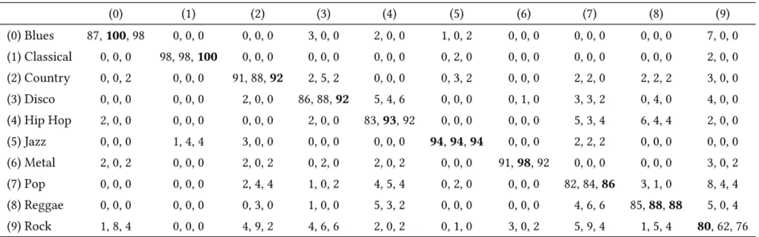
CBMI, June 19-21, 2017, Florence, Italy C.Senac et al. Table 1: Confusion Matrix (in %). Each 3-uple (a, b, c) corresponds to net_STFT (a) , net_MUSIC(b) and Fusion2 (c) results.

(0) (1) (2) (3) (4) (5) (6) (7) (8) (9) (0) Blues 87, 100, 98 0, 0, 0 0, 0, 0 3, 0, 0 2, 0, 0 1, 0, 2 0, 0, 0 0, 0, 0 0, 0, 0 7, 0, 0 (1) Classical 0, 0, 0 98, 98, 100 0, 0, 0 0, 0, 0 0, 0, 0 0, 2, 0 0, 0, 0 0, 0, 0 0, 0, 0 2, 0, 0 (2) Country 0, 0, 2 0, 0, 0 91, 88, 92 2, 5, 2 0, 0, 0 0, 3, 2 0, 0, 0 2, 2, 0 2, 2, 2 3, 0, 0 (3) Disco 0, 0, 0 0, 0, 0 2, 0, 0 86, 88, 92 5, 4, 6 0, 0, 0 0, 1, 0 3, 3, 2 0, 4, 0 4, 0, 0 (4) Hip Hop 2, 0, 0 0, 0, 0 0, 0, 0 2, 0, 0 83, 93, 92 0, 0, 0 0, 0, 0 5, 3, 4 6, 4, 4 2, 0, 0 (5) Jazz 0, 0, 0 1, 4, 4 3, 0, 0 0, 0, 0 0, 0, 0 94, 94, 94 0, 0, 0 2, 2, 2 0, 0, 0 0, 0, 0 (6) Metal 2, 0, 2 0, 0, 0 2, 0, 2 0, 2, 0 2, 0, 2 0, 0, 0 91, 98, 92 0, 0, 0 0, 0, 0 3, 0, 2 (7) Pop 0, 0, 0 0, 0, 0 2, 4, 4 1, 0, 2 4, 5, 4 0, 2, 0 0, 0, 0 82, 84, 86 3, 1, 0 8, 4, 4 (8) Reggae 0, 0, 0 0, 0, 0 0, 3, 0 1, 0, 0 5, 3, 2 0, 0, 0 0, 0, 0 4, 6, 6 85, 88, 88 5, 0, 4 (9) Rock 1, 8, 4 0, 0, 0 4, 9, 2 4, 6, 6 2, 0, 2 0, 1, 0 3, 0, 2 5, 9, 4 1, 5, 4 80, 62, 76

4.4 Results

The mean genre classification accuracies, for cross-validation with 95% confidence intervals computed with bootstrap sampling [4], of the four different systems are reported in table 2.

Table 2: Overall Genre Classification Accuracy (in %). net_STFT net_MUSIC FUSION1 FUSION2

87.8 ± 1.8 89.6 ± 2.4 90.5 ± 0.7 91 ± 1.2 The network net_STFT serves as a baseline and reproduces the results obtained by [23]: it displays an average classification accu-racy of 87.8% ± 1.8. We can see that results obtained with the eight music features are globally superior (89.6% ± 2.4) to those obtained with the spectrogram: this validates the relevance of our features. Finally, the two late fusion systems FUSION1 and FUSION2 have the best rates (91% ± 1.2 for the best one).

The confusion matrices for net_STFT, net_MUSIC and FUSION2 are displayed in table 1. We can notice some complementarity be-tween the first two networks given that the classification errors are not necessarily the same: it can explain why the fusion is efficient. Rock is a problem for both networks, but especially for net_MUSIC: 8% of the rock songs are confused with blues, 9% with country music, 9% with pop music. By fusion, blues and classical are per-fectly recognized and Country, Disco, Hip Hop and Metal obtain an accuracy of 92% at least.

5 CONCLUSIONS

Motivated by the interest of deep learning in the Music Genre Classification task, we decided to use a map of eight musical features as inputs of a CNN. These features were chosen along dynamics, timbre and tonality dimensions, among a larger set studied in an early work. We relied on CNNs trained in such a way that filter dimensions (adapted for our purpose) are interpretable in time and frequency. Results show the relevance of our eight music features: global accuracy of 89.6% against 87.8% for 513 frequency bins of a spectrogram. The late score fusion between systems based on both feature types reaches 91% accuracy on the GTZAN database.

As future work, it is planned to make an early fusion of the two networks in order to have a global classifier. We also have to test our method with other databases with distinct characteristics such as "The Latin American Music database" or ethnic music, on which we have already worked during the DIADEMS project2.

REFERENCES

[1] James Bergstra and Balázs Kégl. 2006. Meta-features and AdaBoost for music classification. In Machine Learning Journal : Special Issue on Machine Learning in Music.

[2] Yandre M.G. Costa, Luiz S. Oliveira, and Carlos N. Silla Jr. 2017. An evaluation of Convolutional Neural Networks for music classification using spectrograms. Applied Soft Computing 52 (2017), 28 – 38. https://doi.org/10.1016/j.asoc.2016.12. 024

[3] Y. M. G. Costa, L. S. Oliveira, A. L. Koerich, F. Gouyon, and J. G. Martins. 2012. Music Genre Classification Using LBP Textural Features. Signal Processing 92, 11 (Nov. 2012), 2723–2737. https://doi.org/10.1016/j.sigpro.2012.04.023

[4] B Efron. 1979. Bootstrap Methods: Another Look at the Jackknife. Ann. Statist. 7, 1 (1979), 1–26.

[5] Xavier Glorot and Yoshua Bengio. 2010. Understanding the difficulty of training deep feedforward neural networks. In Proceedings of the International Confer-ence on Artificial IntelligConfer-ence and Statistics (AISTATS-10). Society for Artificial Intelligence and Statistics.

[6] Xavier Glorot, Antoine Bordes, and Yoshua Bengio. 2011. Deep Sparse Rectifier Neural Networks. In Proceedings of the Fourteenth International Conference on Artificial Intelligence and Statistics (AISTATS-11), Vol. 15. Journal of Machine Learning Research - Workshop and Conference Proceedings, 315–323. [7] A Gray and J Markel. 1974. A spectral-flatness measure for studying the

auto-correlation method of linear prediction of speech analysis. IEEE Transactions on Acoustics, Speech, and Signal Processing 22, 3 (1974), 207–217.

[8] Christopher Harte, Mark Sandler, and Martin Gasser. 2007. Detecting Harmonic Change in Musical Audio. In Proceedings of the 1st ACM Workshop on Audio and Music Computing Multimedia. ACM, NY, USA, 21–26. https://doi.org/10.1145/ 1178723.1178727

[9] Kaiming He, Xiangyu Zhang, Shaoqing Ren, and Jian Sun. 2015. Deep Residual Learning for Image Recognition. CoRR abs/1512.03385 (2015). http://arxiv.org/ abs/1512.03385

[10] Olivier Lartillot, Petri Toiviainen, and Tuomas Eerola. 2006. A Matlab Toolbox for Music Information Retrieval. In Data Analysis, Machine Learning and Applications (Studies in Classification, Data Analysis, and Knowledge Organization). Springer Berlin Heidelberg, 261–268. https://doi.org/10.1007/978-3-540-78246-9_31 [11] Petri Laukka, Patrik Juslin, and Roberto Bresin. 2005. A dimensional approach to

vocal expression of emotion. Cognition and Emotion 19, 5 (2005), 633–653. [12] Thomas Lidy and Alexander Schindler. 2016. Parallel Convolutional Neural

Net-works for Music Genre and Mood Classification. Technical Report. Music Informa-tion Retrieval EvaluaInforma-tion eXchange (MIREX 2016).

[13] Florian Mouret. 2016. Personalized Music Recommendation Based on Audio Features. Master’s thesis. INP ENSEEIHT, Toulouse, France. ftp://ftp.irit.fr/IRIT/SAMOVA/ INTERNSHIPS/florian_mouret_2016.pdf.

(6)

[14] Vinod Nair and Geoffrey E. Hinton. 2010. Rectified Linear Units Improve Re-stricted Boltzmann Machines. In Proceedings of the 27th International Conference on Machine Learning (ICML-10). 807–814.

[15] Loris Nanni, Yandre M.G. Costa, Alessandra Lumini, Moo Young Kim, and Se-ung Ryul Baek. 2016. Combining Visual and Acoustic Features for Music Genre Classification. Expert System Application 45, C (March 2016), 108–117. [16] Jordi Pons, Thomas Lidy, and Xavier Serra. 2016. Experimenting with Musically

Motivated Convolutional Neural Networks. In 14th International Workshop on Content-based Multimedia Indexing (CBMI 2016). IEEE.

[17] William A. Sethares. 2005. Tuning, timbre, spectrum, scale (2nd ed.). Springer, London. https://doi.org/10.1007/1-84628-113-X_2

[18] Claude E Shannon. 1949. W. Weaver The mathematical theory of communication. Urbana: University of Illinois Press 29 (1949).

[19] Bob L. Sturm. 2012. An Analysis of the GTZAN Music Genre Dataset. In Proceed-ings of the Second International ACM Workshop on Music Information Retrieval with User-centered and Multimodal Strategies (MIRUM ’12). ACM, NY, USA, 7–12. [20] Theano Development Team. 2016. Theano: A Python framework for fast

compu-tation of mathematical expressions. arXiv e-prints abs/1605.02688 (May 2016). http://arxiv.org/abs/1605.02688

[21] G. Tzanetakis and P. Cook. 2002. Musical genre classification of audio signals. IEEE Transactions on Speech and Audio Processing 10, 5 (Jul 2002), 293–302. https: //doi.org/10.1109/TSA.2002.800560

[22] Ming-Ju Wu and Jyh-Shing R. Jang. 2015. Combining Acoustic and Multilevel Visual Features for Music Genre Classification. ACM Transactions on Multime-dia Computing Communications and Applications 12, 1, Article 10 (Aug. 2015), 17 pages.

[23] Weibin Zhang, Wenkang Lei, Xiangmin Xu, and Xiaofeng Xing. 2016. Improved Music Genre Classification with Convolutional Neural Networks. In Interspeech 2016, USA, September 8-12. 3304–3308.