HAL Id: hal-00805705
https://hal.inria.fr/hal-00805705
Submitted on 28 Mar 2013
HAL is a multi-disciplinary open access
archive for the deposit and dissemination of
sci-entific research documents, whether they are
pub-lished or not. The documents may come from
teaching and research institutions in France or
abroad, or from public or private research centers.
L’archive ouverte pluridisciplinaire HAL, est
destinée au dépôt et à la diffusion de documents
scientifiques de niveau recherche, publiés ou non,
émanant des établissements d’enseignement et de
recherche français ou étrangers, des laboratoires
publics ou privés.
for Cosparse Signal Modelling
Mehrdad Yaghoobi, Sangnam Nam, Rémi Gribonval, Mike E. Davies
To cite this version:
Mehrdad Yaghoobi, Sangnam Nam, Rémi Gribonval, Mike E. Davies.
Constrained
Overcom-plete Analysis Operator Learning for Cosparse Signal Modelling.
IEEE Transactions on
Sig-nal Processing, Institute of Electrical and Electronics Engineers, 2013, 61 (9), pp.2341-2355.
�10.1109/TSP.2013.2250968�. �hal-00805705�
Constrained Overcomplete Analysis Operator Learning for
Cosparse Signal Modelling
Mehrdad Yaghoobi, Sangnam Nam, R´emi Gribonval and Mike E. Davies
Abstract—We consider the problem of learning a low-dimensional
signal model from a collection of training samples. The mainstream approach would be to learn an overcomplete dictionary to provide good approximations of the training samples using sparse synthesis coefficients. This famous sparse model has a less well known counterpart, in analysis form, called the cosparse analysis model. In this new model, signals are characterised by their parsimony in a transformed domain using an overcomplete (linear) analysis operator. We propose to learn an analysis operator from a training corpus using a constrained optimisation frame-work based on L1 optimisation. The reason for introducing a constraint in the optimisation framework is to exclude trivial solutions. Although there is no final answer here for which constraint is the most relevant constraint, we investigate some conventional constraints in the model adaptation field and use the uniformly normalised tight frame (UNTF) for this purpose. We then derive a practical learning algorithm, based on projected subgradients and Douglas-Rachford splitting technique, and demonstrate its ability to robustly recover a ground truth analysis operator, when provided with a clean training set, of sufficient size. We also find an analysis operator for images, using some noisy cosparse signals, which is indeed a more realistic experiment. As the derived optimisation problem is not a convex program, we often find a local minimum using such variational methods. For two different settings, we provide preliminary theoretical support for the well-posedness of the learning problem, which can be practically used to test the local identifiability conditions of learnt operators.
Index Terms—Sparse Representations, Low-dimensional Signal Model,
Analysis Sparsity, Cosparsity, Dictionary Learning
I. INTRODUCTION
M
ANY natural signals can be modelled using low-dimensional structures. This means, although the investigated signals are distributed in a high dimensional space, they can be represented using just a few parameters in an appropriate model [1]. This is made possible by the fact that few parameters are actually involved in gen-erating/describing such signals. Examples include polyphonic music, speech signals, cartoon images (where some lines/edges describe the images) and standard videos, where the scenes change slightly frame to frame. In modern signal processing, low-dimensional modelling is one of the most effective approaches to clarify the ambiguities in inverse problems, regularise the signals and overcome some conven-tional physical, temporal and computaconven-tional barriers. This model has been heavily investigated in the last decade and many remarkable results achieved in almost all signal processing applications, see for example [2], [3].A natural and crucial question immediately arises. Given a class of signals that we are interested in, how can we model its low-dimensional structures? As an abstract answer, one could imagine that if X ⊂ Rn is the signal class with low-dimensional structures,
then there must be a mapT : Rn
→ Ra
such thatT (x) is sparse for
This work was supported by the EU FP7, FET-Open grant number 225913, the European Research Council - PLEASE project under grant ERC-StG-2011-277906 and EPSRC grants EP/J015180/1 and EP/F039697/1. MED acknowledges support of his position from the Scottish Funding Council and their support of the Joint Research Institute with the Heriot-Watt University as a component part of the Edinburgh Research Partnership.
Copyright (c) 2012 IEEE. Personal use of this material is permitted. However, permission to use this material for any other purposes must be obtained from the IEEE by sending a request to [email protected].
all x∈ X . Unfortunately, finding such T out of all possible maps would be too complex, and one would have to restrict admissible class of maps. A simple option is to consider the class of linear maps. Hence, we ask: is there Ω ∈ Ra×n such that
Ωx is sparse for x∈ X ? This is the type of problem we focus on in this paper. Before getting to the nitty-gritty, we review relevant results to give some contexts to our approach.
A. Sparse Signal Models
The most familiar type of low-dimensional structure is the sparse synthesis model [4], [5].
In this setting, if a signal x∈ Rn
can approximately be generated by adding just a few elementary vectors{di}, called atoms, from an
overcomplete set, called a dictionary, as follows,
x≈X
i∈I
vi"=0
vidi= Dv, (1)
where D∈ Rn×p is the dictionary (matrix) andI is an index set
with small cardinality, i.e.|I| % n, it is called (approximately) sparse
in D. From the signal processing perspective, it is then important to identify the supportI. However, this is not an easy task [6], [7]: when the signals are at mostk-sparse—this means |I| ≤ k—in model (1), they live in a union of subspaces (UoS) model [8], [9], [10] where each subspace has a dimension of at most k, and the number of such subspaces is exponential. A popular and practical approach to find a sparse v is the ℓ1-minimisation [5] in which one looks for
v that minimises 'v'1 among the ones that satisfy x ≈ Dv. The
attractiveness of the ℓ1-objective comes from the fact that it promotes
sparsity and is convex—good in computational aspects—at the same time.
An alternative form of ℓ1-minimisation has been used in practice.
In this form, one looks for x that minimises 'Ωx'1 among the
signals that matches available (linear) information. Here,Ω∈ Ra×n
is some known linear operator. Note that a solution of this ℓ1
-minimisation necessarily leads to many zeros in Ωx and hence is orthogonal to many rows ofΩ (see Figure 1.a). This observation is not exactly compatible with the synthesis interpretation above, and the corresponding low-dimensional model is called the cosparse analysis
model[11]. A signal x in this model is called cosparse.Ω is referred to as the analysis operator in this paper. Although this model is also an instance of the UoS model and relies on the vector form of parsimony, it has many structural differences with the synthesis sparsity model [12], [11]. Very recently the signal recovery using analysis sparsity model has been investigated [13], [11], [14]. As can be deduced from the expressionΩx, the cosparse analysis model is intimately related to our work.
B. Model Adaptation
As can be seen from the synthesis model description, the dictionary D plays an important role. When we deal with the natural signals, one can then naturally ask, how good we can choose such a dictionary? Generally, we can use some signal exemplars [15], [16]
for learning a dictionary or some domain knowledge for designing a suitable dictionary [17], [18]. The readers can refer to [19] and [20] as some surveys on the dictionary selection approaches. It has been shown that the learned dictionaries usually out perform the canonical dictionaries, e.g. DCT and Wavelet, in practice. Online dictionary learning methods [21] have also been introduced to adapt the generative model to a large set of data or a time-varying system. In the exemplar based dictionary learning methods, a set of training signals X∈ Rn×lis given. Similar to sparse approximations, the ℓ
1
norm is often preferred as the sparsity-promoting objective [16], [22], and the dictionary learning with this objective can be formulated as follows: min V,D∈D'V'1+ λ 2'X − DV' 2 F, (2)
where ' · '1 = Pi,j|{·}i,j| and D is an admissible set. Here,
D∈ Rn×p is the dictionary we want to learn and V∈ Rp×l is the coefficient matrix which is expected to be sparse column-wise. The reason for D is to exclude trivial solutions, such as X = DV, with V→ 0 and D → ∞. This type of problem is called the scale
ambi-guityof the signal modelling. Various constraints for the resolution of scale ambiguity have been proposed for dictionaries: fixed atom norms [23], [15], fixed Frobenius norm [24] and convex balls made using these norms [25], [26], [21]. Note that the optimisation (2) is no longer convex and can be difficult to solve. Different techniques have been proposed to find a sensible solution for (2), where they are often based on alternating optimisations of the objective based upon V and D. See [19] and [20] for a review on state of the art methods. Designing (overcomplete) linear transforms to map some classes of signals to another space with a few significant elements, is not a new subject. It has actually been investigated for almost a decade and many harmonic/wavelet type transforms have been designed with some guarantees on fast decay of coefficients in the transform domain (See for example [27] and [28]). These transforms are designed such that the perfect reconstructions of the signals are possible, i.e. bijective mapping.
Relatively few research results have been reported in the exemplar based adaptation of analysis operators. This is an important part of data modelling, which has the potential to improve the performance of many current signal processing applications.
C. Contributions
This paper investigates the problem of learning an analysis operator from a set of exemplars, for cosparse signal modelling. Our approach to analysis operator learning can be viewed as the counterpart to the optimisation (2) in the analysis model setting. Here is the summary of our contributions in this work:
1) We propose to formulate analysis operator learning (AOL) as a constrained optimisation problem. Perhaps surprisingly, in contrast to its synthesis equivalent—the dictionary learn-ing problem—the natural formulation of the analysis operator learning problem as an optimisation problem has trivial solu-tions even when scaling issues are dealt with. The constraints presented in this report exclude such trivial solutions but are also compatible with a number of conventional analysis oper-ators, e.g. curvelets [27] and wave-atoms [28], giving further support for our proposal.
2) We provide a practical optimisation approach for AOL prob-lem, based upon projected subgradient method. Clearly, an AOL principle which does not permit computationally feasible algorithm is of limited value. By implementing a practical algorithm, we also open the possibility to cope with large scale problems.
3) We give preliminary theoretical results toward a character-isation of the local optimality conditions in the proposed constrained optimisation problem. This helps us to better un-derstand the nature of the admissible operator set. It also has potential use in the initialisation of our AOL problem. Our approach is developed from the idea that was primarily suggested in [29] and [30].
D. Related Work
Remarkably, even though the concept of cosparse analysis mod-elling has only been very recently pointed out as distinct from the more standard synthesis sparse model [11], [31], it is already gaining momentum and a few other approaches have already been proposed to learn analysis operators. The most important challenge in formulation of the AOL as an optimisation problem is to avoid various trivial solutions. Ophir et al. used a random cycling approach to statistically avoiding the optimisation problem becoming trapped in a trivial solution [32]. Peyr´e et al. used a geometric constraint, using a linearisation approach, in the operator update step, to get a sensible local optimum for the problem [33]. In a recent approach, Elad et al. have introduced a K-SVD type approach to update each row of the operator at a time [34], [35]. While these approaches have shown promising empirical results, a specificity of our approach is its explicit expression as an optimisation problem.1 We expect
that this will open the door to a better understanding of the AOL problem, through mathematical characterisations of the optima of the considered cost function.
E. Notation and Terminology
In this paper we generally use bold letters for vectors and bold cap-ital letters for matrices. We have presented a list of the most frequent parameters in Table I. We have also presented the corresponding parameters and their range-spaces, used in the related papers, in the same table. The notation ( · )i,j, or simply subscript i,j, has been
used to specify the element locating in theith
row andjth
column of the operand matrix.' · '1,' · '2and' · 'F are respectively ℓ1, ℓ2
and Frobenius norms. With an abuse of notations, we will use' · '1
for the norm defined by the entrywise sum of absolute values of the operand matrix, which is different from the ℓ1 operator norm for
matrices. The notation* , + represents the canonical inner-product of two operands for, respectively, ℓ2and Frobenius norms, in the
vector-valued and matrix-vector-valued vector spaces.tr{·} denotes the trace of the operand matrix. The notation P will be used to represent the orthogonal projection whose range is specified by the subscript, e.g. PU N. Sub- and super- scripts in braces are used to indicate iteration
number in the algorithm section.
The sparsity of x in D is noted here byk, which is the cardinality of the support of v, where v is the sparse representation of x. We can similarly define the cosparsity of x [31], with respect toΩ, and note it byq, which is the cardinality of its co-support, i.e. co-support(x) = {i : 1 ≤ i ≤ a, {Ωx}i= 0}.
Following the notation of [36], a sub-indexed vector or matrix will be determined using a subscript for the original parameter, e.g. ΩΛ. Here,ΩΛhas the dimension ofΩ, identical values as Ω in its
supportΛ and zeros elsewhere. We also use “bar”, e.g. ¯Λ, to denote a complement of the index setΛ in this context.
1Peyr´e and Fadili [33] use a similar type of expression to learn an analysis operator in the context of signal denoising, with exemplars of noisy and clean signals.
TABLE I
THE NOTATION OF CURRENT AND THEIR CORRESPONDING NOTATIONS IN RELATED PAPERS.
This paper PF[33] RFE [35] (OEBP[32]) Observation y ∈ Rn y ∈ RN y ∈ Rd Signal x ∈ Rn x ∈ RN x ∈ Rd Analysis vector z ∈ Ra - -Dictionary D ∈ Rn×p D ∈ RN×P D ∈ Rd×n Synthesis vector v ∈ Rp u ∈ RP z ∈ Rn Analysis operator Ω ∈ Ra×n D∗∈RP×N Ω ∈ Rp×d
Training size l n R (N )
Cosparsity q - l
Sparsity k - k
F. Organisation of the Paper
In the following section, we formulate the analysis operator learning problem as a constrained optimisation problem. We briefly review some of canonical constraints for the exemplar based learning frameworks and explain why they are not enough. we introduce a new constraint to make the problem ‘well-posed’ in II-B4. After the formulation of the AOL optimisation problem, we introduce a practical algorithm to find a sub-optimal solution for the problem in section III. Following the algorithm, in Section IV, we will present some simulation results for analysis operator learning with different settings. The simulations are essentially based on two scenarios, synthetic operators and operators for image patches. In the appendix, we will investigate the local optimality conditions of operators for the proposed learning framework.
II. ANALYSISOPERATORLEARNINGFORMULATION
The aim of analysis operator learning is to find an operator Ω adapted to a set of observations of the signals yi:= M(xi), where
xi is an element (column) of sample data X∈ Rn×l and M(xi)
denotes the information available for the learning algorithm. For our purposes, we set M(xi) := xi+ ni, where ni ∈ Rm denotes the
(potential) noise. The data X is assumed to be of full rankn since otherwise, we can reduce the dimension of the problem with a suitable orthogonal transform and solve the operator learning in the new low dimension space.
A standard approach for these types of model adaptation problems, is to define a relevant optimisation problem such that its optimal solution promotes maximal sparsity of Z := ΩX. The penalty ' · 'p := P | · |p, 0 < p ≤ 1 can be used as the sparsity promoting
cost function. As hinted in the introduction, we will use the convex ℓ1 penalty. The extension to an ℓp, p < 1, AOL is left for a future
work.
A. Constrained Analysis Operator Learning (CAOL)
Momentarily assume that we know X. Unconstrained minimisation of 'ΩX'1, based on Ω, has some trivial solutions. A solution for
such a minimisation problem is Ω = 0! A suggestion to exclude such trivial solutions is to restrict the solution set to an admissible setC.
Not assuming that X is known any more, AOL can thus be formulated as,
min
Ω,X'ΩX'1, s. t. Ω ∈ C, 'Y − X'F ≤ σ (3)
where σ is the parameter corresponding to the noise. We call the AOL to be a noiseless operator learning when σ= 0.
!"# !$#
!%# !&#
Fig. 1. Data clouds around some union of subspaces and possible analysis operators: a) an ideal operator, b) the optimal (rank-one) operator using a row norm constraint, c) the optimal operator using the full-rank, row norm constraint and d) the optimal operator using tight frame constraint.
We prefer to use an alternative, regularised version of (3), using a Lagrangian multiplier λ, to simplify its optimisation. The reformu-lated AOL is the following problem,
min Ω,X'ΩX'1+ λ 2'Y − X' 2 F, s. t. Ω ∈ C (4)
If λ → ∞, problem (4) is similar to the noiseless case. In the following section, we explore some candidates forC.
B. Constraints for the Analysis Operators
A suitable admissible set should exclude undesired solutions of AOL while minimally affecting the rest of the search space. We name Ω = 0 and Rank{Ω} = 1 as some undesired solutions of (3). These operators clearly do not reveal low-dimensional structures of the signals of interest. For simplicity, we again assume that X is given, i.e σ= 0.
Here, we intially propose some constraints for the problem (3) and explain why some of them can not individually exclude undesired solutions. A combined constraintC, which is the Uniform Normalised Tight Frame (UNTF), will be introduced subsequently. The proposed constraint is smooth and differentiable.
1) Row norm constraints are insufficient: The first constraint is on the norms of rows ofΩ, i.e.'ωi' = c for the ith row. We can
find the solution of the optimisation by first finding ω∗ ∈ Rn
that minimises'ωT
X'1. Then, the optimum is obtained by repeating ω∗,
i.e.,Ω∗1:= [ωi= ω]Ti∈[1,a]is the minimum. Of course,Rank{Ω∗1} =
1 (see Figure 1.b), and the solution is not interesting enough.
2) Row norm + full rank constraints are insufficient: The setCF
of full rank operators is not closed, and the operatorΩ∗1 belongs to
its closure. As a result, the problem (3) with σ= 0 does not admit a minimiser but there is a sequence of operators, arbitrarily close to Ω∗1, that yield an objective function arbitrarily close to its infimum
value.
3) Tight frame constraints are insufficient: In a complete setting a = n, an orthonormality constraint can resolve the ill-conditioning of the problem. The rows of Ω are geometrically as separated as
possible. Letting a > n, the orthonormality constraint is not further applicable, i.e. more rows than the dimension of space. In this case, the orthonormality constraint in the ambient space, ∀i -= j, ωi
⊥ωj
and 'ωi
'2 = 'ωj'2 = 1, where ωiand ωj ∈ Ra are respectively
the ith
and jth
columns of Ω, is possible. The admissible set of this constraint is the set of tight frames in Ra×n, i.e. ΩT
Ω = I, where I is the identity operator in Rn. The admissible setC = {Ω ∈ Ra×n: ΩT
Ω = I} is smooth and differentiable, which is a useful property for optimisation over this set. Such a constraint actually constructs a manifold in the space of Ra×n, called the (orthogonal) Stiefel manifoldSt(a, n) [37].
Although the tight frame constraint may look appropriate to avoid “trivial” solutions to (3), preliminary empirical and theoretical investigations indicate that the analysis operator minimising (3), using this constraint, is always an orthonormal basis completed by zero columns (see Figure 1.d). This is possibly caused by the fact that the zero elements in such operators, are orthogonal to all finite signals, without giving any insight about their directions, and the operators can thus be truncated to produce complete operators. Therefore, this constraint does not bring anything new compared to the orthonormality constraint.
4) Proposed constraint: Uniform Normalised Tight Frame: This motivates us to apply an extra constraint. Here, we choose to combine the uniformly normalised rows and the tight frame constraints, yielding the UNTF constraint set. This constraint will be used in the rest of paper and the analysis of Appendix A is based on this admissible set.
The UNTF’s are actually in the intersection of two manifolds, uniform normalised (UN) frames manifold and tight frames (TF) manifold. There exist some results that guarantee the existence of such tight frames, i.e. non-emptiness of the intersection of two manifolds, for any arbitrary dimensionsn and a [38]. This is indeed an important fact, as the optimisation with such a constraint is then
always feasible.
This constraint can be written as follows, C = {Ω ∈ Ra×n : ΩT
Ω = I, ∀i 'ωi'2= c}, (5)
and ωiis theith row of Ω. Since C is not convex, (4) may have many
separate local optima. Finding a global optima of (4) is not easy and we often find a local optima using variational methods. Using variational analysis techniques, we can also check if an operatorΩ is a local optimum. Details are presented in Appendix A.
The exact recovery, using a variational analysis, in this setting, is essentially based on the following property,
Definition 1 (Locally Identifiable): An operatorΩ is locally iden-tifiable from some (possibly noisy) training cosparse signals Y, if it is a local minimum of an optimisation problem with a continuous objective and locally connected constraint.
This definition of local identifiability is a generalisation of the (global) identifiability as here we can not find the global solution. Such a property has been previously investigated in the context of dictionary learning in [36] and [39].
C. Extension of UNTF Constraints
In some situations, we may not necessarily want to require that Ω form a frame for the whole of Rn. The inspiration for such a case comes from the finite difference operators which is closely tied to the popular TV-norm. When we model cartoon-like piece-wise constant images, an analysis operator Ω need only to detect transitions in neighboring pixel values. Therefore, all the rows ofΩ can be orthogonal to the DC component.
We can facilitate learning similar rank-deficient operators by ex-tending the UNTF constraints. Here, we know thatΩ⊥ N , where N is the known null-space. We can modify (5) to construct the following constraint,
CN= {Ω ∈ Ra×n : ΩTΩ = PN ⊥, ∀i 'ωi'2= c}, (6)
wherePN ⊥ is the orthogonal projection operator onto the span of
N⊥.
In the following, we introduce a practical algorithm to find a suboptimal solution of (4), constrained toC or CN, using a projected
subgradient based algorithm.
III. CONSTRAINEDANALYSISOPERATORLEARNING
ALGORITHM
Cosparse signals, by definition, have a large number of zero ele-ments in the analysis space. In this framework, a convex formulation for recovering a signal x from its (noisy) observation is to minimise the following convex program,
min x 'Ωx'1+ λ 2'y − x' 2 2, (7)
where Ω is a fixed analysis operator. As (7) is a convex problem, many algorithms have been proposed to solve this program very efficiently (see [40],[41] and [42] as some examples of the latest methods). These methods can easily be extended to the matrix form to find X given Y. Unfortunately, the AOL problem (4), due to the freedom to also changeΩ∈ C in this formulation, is very difficult.
This difficulty is similar to what we face in the dictionary learning for synthesis sparse approximation. In the dictionary learning prob-lem, we have also a joint optimisation problem (2) that, in a simple setting, can be minimised in an alternating optimisation approach [43] as follows,
Dictionary Learning:
initialisation: D[0], V[0]= 0, i = 0,
while not converged do
V[i+1]= argminV'V'1+λ2'X − D[i]V'2F,
D[i+1]= argminD∈D'X − DV[i+1]'2F
i = i + 1
end while.
An alternating minimisation technique can also be used for the AOL problem to seek a local minimum. In this framework we first keep X fixed and update the operator Ω. We then update the cosparse approximations of the signals while keeping the operator fixed. Such an alternating update continues while the new pair (X, Ω) is very similar to the previous (X, Ω) or is repeated for a predetermined number of iterations. A pseudocode for such an alternating minimisation AOL is presented in Algorithm 1, Analysis Operator Learning Algorithm (AOLA). Each subproblem, i.e line 3 or line 4, of AOLA can be solved separately based upon a single parameter. Although the problem in line 4 is convex and it can thus be solved in a polynomial time, the problem in line 3 is not a convex problem due to the UNTF constraintC.
Note that when the cosparse matrix X is given, i.e. in a noiseless scenario σ = 0, the algorithm only has the operator update step, which we need to repeat until convergence. This step is also called noiseless AOL[29].
A. Analysis Operator Update
We use a projected subgradient type algorithm to solve the operator update subproblem in line 3 of the AOLA. The subgradient of the
Algorithm 1 Analysis Operator Learning Algorithm (AOLA)
1: initialisation:Ω[0], X[0]= Y, i = 0,
2: while not converged do
3: Ω[i+1]= argminΩ∈C'ΩX[i]' 1, 4: X[i+1]= argminX'Ω [i+1]X '1+λ2'Y − X'2F 5: i = i + 1 6: end while.
objective is ∂f (Ω) = sgn(ΩX[i])X[i]T, where sgn is an extended set-valued sign function defined as follows,
{sgn(A)}i j =sgn(Ai j) sgn(a) = 8 > < > : 1 a> 0, [−1, 1] a = 0, −1 a< 0.
In the projected subgradient methods, we have to choose a value in the set of subgradients. We randomly choose a value in[−1, 1], when the corresponding element is zero.
After the subgradient descent step, the modified analysis operator is no longer UNTF and needs to be projected onto the UNTF set. Unfortunately, to the authors’ knowledge, there is no analytical method to find the projection of a point onto this set. Many attempts have been done to find such an (approximate) projection, see for example [44] for an alternating projections and [45] for an ordinary differential equations based method. We rely on an alternating pro-jections approach.
Projection of an operator with non-zero rows, onto the space of fixed row norm frames is easy and can be done by scaling each row to have normc. We use PU N to denote this projection. If a row is
zero, we set the row to a normalised random vector. This means that PU N is not uniquely defined. This is due to the fact that the set of
uniformly normalised vectors is not convex. The projection can be found by, PU N{Ω} = [PU N{ωi}]i, PU N{ω} := ( ω &ω&2 'ω'2-= 0 ν otherwise, where ν is a random vector on the unit sphere.
Projection of a full rank matrix onto the tight frame manifold is possible by calculating a singular value decomposition of the linear operator [44]. LetΩ∈ Ra×nbe the given point and
Ω = UΣVT be
a singular value decomposition ofΩ and Ia×nbe a diagonal matrix
with identity on the main diagonal. The projection ofΩ can be found using,
PT F{Ω} = U Ia×nV T
.
Note that, although there is no guarantee to converge to a UNTF using this method, this technique practically works very well [44]. As the projected subgradient continuously changes the current point, which needs to be projected onto UNTF’s, we only use a single pair of projections at each iteration of the algorithm, to reduce the complexity of the algorithm, where the algorithm now asymptotically converges to a UNTF fixed point. To guarantee a uniform reduction of the objective f (Ω), we can use a simple line search technique to adaptively reduce the stepsize. It indeed prevents any large update, which increasesf2 . A pseudocode of this algorithm is presented in
Algorithm 2, whereKmax is the maximum number of iterations.
2The stability of algorithm is guaranteed in a Lyapunov sense, i.e. the operator Ω[k]is enforced to remain bounded, when k → ∞.
Algorithm 2 Projected Subgradient Based Analysis Operator Update Input: X[i],Kmax,Ω[i], η, (% 1, ρ < 1,
initialisation:k = 1, Ω[0]= 0, Ω[1]= Ω[i]
while(≤ 'Ω[k]− Ω[k−1]'F andk ≤ Kmaxdo
ΩG∈ ∂f(Ω[k]) = sgn(Ω[k]X[i])X[i] T Ω[k+1]= PU N{PT F{Ω[k]− η ΩG}} whilef (Ω[k+1]) > f (Ω[k]) do η= ρ.η Ω[k+1]= PU N{PT F{Ω[k]− η ΩG}} end while k = k + 1 end while output:Ω[i+1]= Ω[k−1]
For the constraint set CN mentioned in Section II-C, we present
a simple modification to the previous algorithm in order to constrain the operator to have a specific null-space. Here, we need to find a method to (approximately) project an operator ontoCN. Following
the alternating projection technique, which was used earlier to project ontoC, we only need to find the projection onto the set {Ω ∈ Ra×n : ΩT
Ω = PN ⊥}, as we already know how to project onto UN, i.e.
PU N. To project an Ω onto the set of TF’s in N⊥, we need to
compute the singular value decomposition of Ω, projected into the orthogonal complement space ofN . The projection onto N⊥,P
N ⊥,
can be found using an arbitrary orthonormal basis forN and simply subtracting the projection onto this basis, from the original Ω. We can then rewrite the decomposition asPN ⊥{Ω} = U Σ V
T. If the
dimension ofN is r, only n − r singular values of PN ⊥{Ω} can be non-zero. We find the constrained projection as follows,
PT F⊥N{Ω} = U Ira×nV T
,
where matrix Ira×n is a diagonal matrix in Ra×n, with identity
values on the firstn − r diagonal positions, while the last r elements are set to zero.
We therefore need to alternatingly usePT F⊥N and PU N to find
a point in the intersection of these two constraint sets. In Algorithm 2, we only need to replacePT F withPT F⊥N to consider the new
constraintCN.
B. Cosparse Signal Update
WhenΩ is known or given by line 3 of AOLA, a convex program based on X needs to be solved. Although this program is a matrix valued optimisation problem, it can easily be decoupled to some vector valued subproblems based upon the columns of X. One approach is to individually solve each subproblem. Here we present an efficient approach to solve this program in the original matrix-valued form, despite the challenging nature of it, due to its large size.
The main difficulties are, a) ℓ1is not differentiable and b)Ω inside
the ℓ1 penalty, does not allow us to use conventional methods for
solving similar ℓ1 penalised problems. We here use the
Douglas-Rachford Splitting (DRS) technique to efficiently solve the cosparse signal approximation of the AOLA. It is also called the alternating direction method of multipliers (ADMM) in this setting, see [46] for a brief overview. This technique has indeed been used for the Total Variation (TV) and analysis sparse approximations in [40][47]3. We here only present a simple version of the DRS technique, carefully
3[47] derives the formulation by incorporating the Bregman distance. However, it has been shown that the new method, called Alternating Bregman Splitting method, is the same as DRS, applied to the dual problems [48].
Algorithm 3 DRS Based Cosparse Signal Update Input:i, Ω[i+1],K
max, X[i], γ, λ, (% 1, λ, γ
1: initialisation:k = 1, X[k]= X[i],Ω = Ω[i+1], B[k]= 0,
Z[k]= ΩX[k]
2: while(≤ 'X[k]− X[k−1]'F andk ≤ Kmax do 3: X[k+1]= (λI + γΩTΩ)−1(λY + γΩT(Z[k]− B[k])) 4: Z[k+1]= S1 γ ˘ ΩX[k+1]+ B[k] ¯ 5: B[k+1]= B[k]+ (ΩX[k+1]− Z[k+1]) 6: k = k + 1 7: end while 8: output: X[i+1]= X[k−1]
tailored for this problem. The problem is a constrained convex program with two parameters Z= Ω[i+1]X and X as follows,
min X,Z'Z'1+ λ 2'Y − X' 2 F s. t. Z = Ω [i+1] X. (8)
The Augmented Lagrangian (AL) [49] method is applied to solve (8). In the Lagrangian multiplier method we use the dual parameter B∈ Ra×l and add a penalty term,DB, Ω[i+1]X− ZE. In the AL,
we also add an extra quadratic penalty related to the constraint and derive the new objective g(X, Z, B) as follows,
g(X, Z, B) ='Z'1+λ 2'Y − X' 2 F + γ D B, Ω[i+1]X− ZE +γ 2'Ω [i+1] X− Z'2F ='Z'1+λ 2'Y − X' 2 F + γ 2'B + Ω [i+1] X− Z'2F −γ2'B'2F,
where 0 < γ ∈ R+ is a constant parameter. According to the duality property, the solution ofmaxBminX,Zg(X, Z, B) coincides
with the solution of (8). Using the DRS method, we iteratively optimise a convex/concave surrogate objectivegs(X, Z, B, B[k]) =
g(X, Z, B)−'B−B[k]'2F, where B[k]is the current estimation of B.
The fixed points of the iterative updates ofgs(X, Z, B, B[k]) are the
same asg(X, Z, B), as the extra term 'B − B[k]'2F vanishes in any
fixed points.gs(X, Z, B, B[k]) is convex with respect to Z and X and
concave with respect to B. We can thus iteratively update each of the parameters, while keeping the rest fixed, see Algorithm 3. In this al-gorithm,Sα, with an α> 0 , is the entrywise soft-threshold operator
defined bySα(β) = β − α sgn(β) if |β| ≥ α and 0 otherwise [50].
Note that the update formula for X in Algorithm 3, line 3, involves a matrix inversion, which is computationally expensive. AsΩ is a tight frame here, the matrix inversion is significantly simplified using the fact thatΩT
Ω is identity. In this case, the operator (λI+ γ ΩT
Ω)−1 is simply a scaling with λ+γ1 .
We iterate Algorithm 3 for a number of iterationsKmaxor until the
parameters cease to change significantly. Although the convergence of the iterative updates of this algorithm can separately be investigated, it can also be deduced using the fact that it is a particular case of DRS, which converges under mild conditions [46].
IV. SIMULATIONS
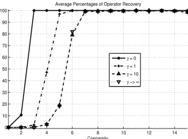
We present two categories of simulation results in this section. The first part is concerned with empirical demonstration of (almost) exact recovery of the reference analysis operators. An astute reader might ask: why should we care about exact recovery at all? Is it not enough to show that learned operators are good? This is, of course, true. However, when the signals are generated to be cosparse with respect to a reference operator or they are known to be cosparse
2 4 6 8 10 12 14 0 10 20 30 40 50 60 70 80 90 100 Cosparsity
Average Percentages of Operator Recovery
γ = 0 γ = 1 γ = 10 γ −> ∞
Fig. 2. The average percentage of operator recovery for different γ’s, where γ controls how far is the starting point ΩinformΩ0. The x-axis presents
the cosparsity of the synthetic data.
with respect to a known analysis operator, the recovery of those operators is a good demonstration of the effectiveness of our method. Going further, one may imagine situations where the rows of the reference analysis operators explain certain properties/dynamics of the signals; for example, finite differences for piecewise constant images detect edges. Obviously, the recovery of reference operators in these contexts is significant.
In the second part, we are interested in demonstrating the effective-ness of learned operators in a practical task, namely, image denoising.
A. Exact recovery of analysis operators
For the first experiment, the reference operators and the cosparse signal data set were generated as follows: A random operatorΩ0−∈
R24×16
was generated using i.i.d. zero mean, unit variance normal random variables4. The reference analysis operator Ω0 is made by
alternatingly projecting Ω0− onto the sets of U N ’s and T F ’s. A
set of training samples was generated, with different cosparsities, by randomly selecting a normal vector in the orthogonal complement space of a randomly selectedq rows of Ω0. Such a vector yihas (at
least)q zero components in Ω0yi, and it is, thus,q cosparse.
To initialise the proposed algorithm, we used a linear model to generate the initialΩ by combining the reference operator Ω0 and
a normalised random matrix N, i.e. Ωin = Ω0+ γ N, and then
alternatingly projecting ontoU N and T F . It is clear that when γ is zero, we actually initialiseΩ with the reference model Ω0and when
γ→ ∞, the initial Ωinwill be random.
First, we chose a set of sizel = 768 of such training corpus and used the noiseless formulation (3), where σ= 0. The AOL algorithm in this setting is just the projected subgradient base algorithm, Algorithm 2, which was iterated 50000 times. To check the local optimality of the operator and the size of basin of attraction, we chose γ= 0, 1, 10 and ∞. The average percentage of operator (rows) recovery, i.e. the maximum ℓ2 distance of any recovered row and
the closest row of the reference operator, is not more than √.001, for different cosparsity and 100 trials, are plotted in Figure 2. We practically observe that the operator is the local optimum even when the cosparsity of the signal is as low as 3. We also see that the average recovery reduces by starting from a point far from the the actual reference operator or a random operator, which is the case γ→ ∞.
4Ω
0−is not necessarily a UNTF and needs to be projected onto the set of
2 4 6 0 50 100 l = 384 γ = 0 2 4 6 0 50 100 γ = 1 2 4 6 0 50 100 γ = 10 2 4 6 0 50 100 l = 768 2 4 6 0 50 100 2 4 6 0 50 100 2 4 6 0 50 100 l = 1536 2 4 6 0 50 100 2 4 6 0 50 100
Fig. 3. The average percentage of operator recovery with different training set population size l. The x-axis presents the cosparsity of the signals.
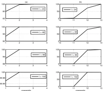
1 2 3 4 60 80 100 (a) 10 11 12 13 0 50 100 (b) 1 2 3 4 90 95 100 10 11 12 13 0 50 100 1 2 3 4 98 99 100 10 11 12 13 0 50 100 1 2 3 4 99.96 99.98 100 cosparsity 10 11 12 13 0 50 100 cosparsity l = 24 l = 24 l = 48 l = 48 l = 96 l = 96 l = 192 l = 192
Fig. 4. The local-identifiability check by randomly generating vectors in the admissible set of Lemma 3 of Appendix A and checking the credibility of the inequality in (a) Lemma 3- Equation (17); and (b) Theorem 1- Equation (18).
We now investigate the role ofl on the average operator recovery by some simulations. We kept the previous experiment settings and repeated the simulations for two new training sets, with populations ofl = 384 and 1536, which are 1/2 and 2 times of the population in the previous experiments. We show the average operator recovery for γ= 0, 1, 10 in Figure 3. The simulation results show not only that Ω0can be locally identified with even less cosparse signals, smaller
q, but the basin of attraction is also extended and now the reference operator can be recovered by starting from a distant initial point, even using 2 cosparse signals.
In the next two experiments, we show that if the cosparsity is low, i.e. small q, then the analysis operator cannot be “recovered”: it is not a solution of the proposed optimization problem (3). One way to demonstrate it would consist in solving the large scale convex optimisation program (15) expressed in Proposition 2 of the Appendix A. Alternatively, we can use Lemma 3 (respectively Theorem 1) of the
Fig. 5. A 512 by 512 Shepp-Logan phantom image which was used as the training image.
2−times Overcomplete Haar Operator Full−rank
Learned Operator Learned OperatorRank−deficient
Fig. 6. The rows of the full-rank learned operator (left panel), the rank-deficient learned operator (middle panel) and a two-times oevrcomplete Haar operator (right panel), in the form of 8 by 8 blocks.
appendix, to possibly find a matrix∆z, which violates the conditions.
Here, we randomly generated 1000∆z inTCs, and checked whether
the inequality (17) (respectively (18)) was satisfied. We repeated this process for 10 different pseudo-randomly generatedΩ and plotted the percentages of∆z satisfying the inequality in Figure 4, respectively
in the left column (a) and the right column (b). We have also mentioned the training size, i.e.l on each row of this figure. From left column, we can see that with 1-cosparse signals, there are operators which are not local minimum of the program (3) (σ= 0). We can also see that the relaxation used to derive Theorem 1, makes the result of this Theorem very conservative, i.e. there are many cases which do not satisfy this theorem, but they still can be locally-identifiable. For the last experiment, we chose the Shepp Logan Phantom, a well-known piecewise constant image in the Magnetic Resonance Imaging (MRI) community (see Figure 5). We usedl = 16384 blocks of size 8 by 8, randomly selected from the image, such that, except one DC training sample, all the training images contain some edges. We learned a 128 × 64 operator for the vectorised training image patches, by initialising the (noise-less) AOL algorithm with a pseudo-random UNTF operator. We used two different constraintsC and CN
for the learning operator Ω, i.e. (5) and (6), where the null space was selected to be constant images. We chose the second constraint to see if we would find a different operator by enforcing a similar null-space to the Finite Difference (FD) operator.
The learned operators are shown in Figure 6. We found operators which have many FD type elements. The operator which we learned usingC in (6) seems to have more FD type elements. We also compare
0 1 2 3 4 5 6 7 8 9 10 x 104 105.3 105.4 105.5 Iteration || Ω Y || 1 Learned Operator 2X Haar Operator
Fig. 7. The value of objective in (14), in comparison with a base line, i.e. the objective value with a two times overcomplete Haar wavelet operator.
0 20 40 60 80 100 120 −20 0 20 N − || Ω0 y || 0 = 0 (a) 0 20 40 60 80 100 120 −20 0 20 N − || Ω y || 0 = 1 (b) 0 20 40 60 80 100 120 −10 0 10 N − || Ω y ~||0 = 27 (c)
Fig. 8. Signals in the analysis space RN, N = 128. The coefficients with almost zero magnitude, i.e. less than 0.01, are indicated with stars. The cosparsity in each case is: (a) p = 0, (b) p = 1, and (c) p = 27.
the level of objective value for the learned operator, usingC in (5), and a reference operator. As a two dimensional FD operator is not a UNTF, we chose a two-times overcomplete Haar wavelet—see the right panel of Figure 6—which has some similarities with the FD, in the fine scale. The objective of (4) for the learned operator in different steps of training and the Haar based operator are shown in Figure 7. This shows that the learned operator finally outperforms the baseline operator in the objective value. Note that if we initialise the algorithm with the Haar based operator, the AOL algorithm does not provide a new operator. This empirically shows that the reference operator is a local optimum for the problem (4), where λ → ∞. This fact can be investigated using the analysis provided in Appendix A, i.e. randomly generating admissible vectors and checking (17) or (18).
B. Image denoising with learned analysis operators
For the next experiments we used a set of face images which are centred and cropped [51]. Such images can be modelled as ap-proximately piecewise smooth signals. A pseudo-random admissible Ω[0] ∈ R128×64 has been used as an initial analysis operator and a training set of size l = 16384 of 8 × 8 image patches from 13 different faces, after normalised to have mean zero, have been used to learn the operators (a = 128).
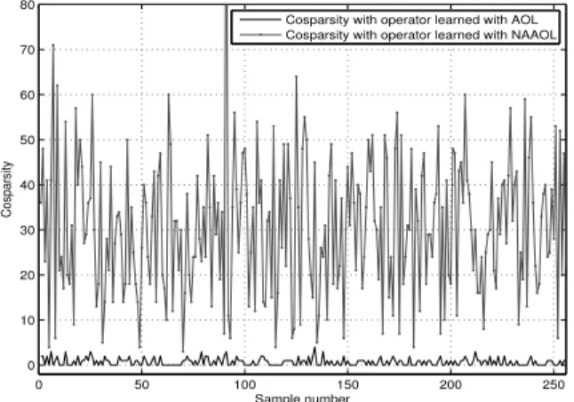
We applied both of the noiseless AOL Algorithm and the noise-aware AOL Algorithm to demonstrate how much the cosparsities of the training samples increase using the noise aware formulation. (NL)AOL algorithm was iteratedKmax= 100000 times and NAAOL
0 50 100 150 200 250 0 10 20 30 40 50 60 70 80 Sample number Cosparsity
Cosparsity with operator learned with AOL Cosparsity with operator learned with NAAOL
Fig. 9. The cosparsities of y (bottom plot) and yb(top plot) respectively with the operators learned with (NL)AOL and NAAOL.
algorithm iterated forKmax= 10 iterations with λ = γ = 0.5, while
the inner-loop, i.e. Algorithm 2, was iterated 100000 times. A plot of the analysis coefficients for a selected y along with its corresponding cosparsities, with three differentΩ’s, are presented in Figure 8. The initial operatorΩ0 = Ω[0] has been applied to y in
(a). Not surprisingly, the signal is not cosparse with this arbitrary operator (q = 0). In (b), the same plot is drawn using the learned operator with (NL)AOL. Although some coefficients are small, most are not zero, andq = 1. In the last plot, we have shown the analysis coefficients for x using the learned operator with NAAOL. It is clear that the cosparsity has been increased significantly (from q = 1 to q = 27). We have further plotted the cosparsities of the first 256 training samples y’s using the learned operator found by (NL)AOL and corresponding approximations x’s, which are found by NAAOL, in Figure 9. This figure also shows, the operator learning using the noise aware formulation (4), where λ is finite, results in much greater cosparsity. We show the learned operator found using NAAOL algorithm in Figure 10. This experiment suggests that a harmonic type operator should perform better than FD based operators for such images. This is an interesting observation which should be explored in the future in more detail.
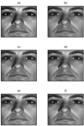
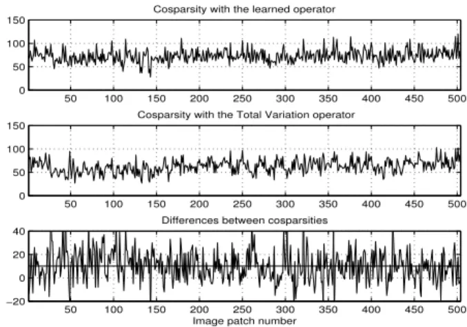
The aim of next experiment is to compare denoising performance of an image using a learned operator and a FD operator [52] which is similar to the analysis operator in the TV denoising formulation and is shown in the right panel of Figure 10). We keep the previous experiment settings. The learned operator and the FD operator can now be used to denoise a corrupted version of another face from the database, using (7). The original face is shown in Figure 11 (a) and the noisy version, with additive i.i.d Gaussian noise, is shown in (b), with PSNR = 26.8720 dB. Denoising was performed using two different regularisation settings:(λ = γ) = 0.3, 0.1. The bottom two rows show the denoised images using the FD operator and the learned operator. We can visually conclude that the two operators successfully denoise the corrupted images with some slight differences. The results with the learned operators are smoother (this is mostly visible on a screen rather than a printed copy of the paper). The average PSNR’s of the denoised images over 100 trials are presented in Table II. Although we get a marginally better average PSNR using the learned operator instead of FD when λ = 0.3, we get a noticeably better average PSNR, i.e., 1 dB, when λ= 0.1.
As the initial goal was to increase the cosparsities of signals, we have also shown the cosparsities of different patches of the selected face image (see Figure 12). The horizontal axis presents the index number of the patches. To compare the cosparsity using these operators, we have plotted their differences and its average in
TABLE II
AVERAGEPSNR (DB)OF THE DENOISED FACE IMAGES(100TRIALS)
USING,A) FDAND B)THE LEARNED OPERATORS,WHEN THE AVERAGE
PSNROF THE GIVEN NOISY IMAGES WAS26.8720DB λ = 0.3 λ = 0.1 Finite Difference 28.9643 31.5775 Learned Operators 29.0254 32.5202
TABLE III
AVERAGEPSNR (DB)OF THE DENOISED FACE IMAGES(5TRIALS),WHEN THE AVERAGEPSNROF THE GIVEN NOISY IMAGES WAS APPROXIMATELY
26.6DB (VARIES SLIGHTLY IN DIFFERENT EXPERIMENTS) Synthesis (OMP) Analysis (ℓ1)
DCT 34.63 31.6
Learned 34.87 34.22
the bottom plot. Positive values here demonstrate the cases when the learned operator is a better operator than the FD operator. The average, which is indeed positive, is plotted as a horizontal line. As a result, the learned operator here performs much better (15% improvement) than the FD operator.
The synthesis framework has been used for different applications with some very promising results. In the last experiment, we have a comparative study between the two frameworks, for denoising face images. We chose the settings of the previous experiment and used the patch based learning. For the reference, we used a two times overcomplete DCT, which is a standard selection for the sparsity based denoising [53]. For the synthesis sparse representation, we used OMP method, and for the analysis sparse recovery, we used a convex formulation similar to the previous experiment. The optimum value of λ in the ℓ1 analysis was 0.04. The OMP was running
to achieve an approximation error equal to 1.15σ, where σ is the standard deviation of the additive noise. This setting has been used in [53], for denoising with the learned synthesis dictionary using K-SVD method. We used another technique, which has also been used in the mentioned reference, to average out over the overlapping-blocks of images to reduce the blocking effect. The average PSNR’s of the denoised face images over 5 trials, for the DCT dictionary/operator are shown in the first row of Table III.
This experiment demonstrates that the synthesis framework works better in the denoising of face images. We already have techniques to learn dictionaries/operators for each of these three cases. For the OMP and analysis based denoisings, we respectively chose K-SVD [54] and the proposed CAOL methods. The Lagrange multiplier for the analysis based denoising was λ = 0.09, while we used the operator learned in the previous experiment. The average PSNR’s of the denoised face images over 5 trials are presented in the second row of Table III.
By comparing the synthesis denoising techniques, with the over-complete DCT and K-SVD dictionaries, we find a slight improvement (+0.2 dB) in the PSNR of the denoised images, using the learned dictionary. This improvement is more significant in the analysis denoising framework, as we achieved more than 2.5 dB improvement in the PSNR of the denoised image. In comparison between two frameworks, although the PSNR of the denoised image using the learned operator is significantly improved, it is marginally behind the synthesis competitor. However, we found these results very promising, since this is only the beginning of the field “denoising with the learned analysis operators”. More experiments are necessary to find a reason for such a behaviour, which we leave it for the future work.
Fig. 10. The learned analysis operator in a noisy setting, λ = 0.1 (left panel) and the finite difference operator (right panel).
(a) (b)
(c) (d)
(e) (f)
Fig. 11. Face image denoising. Top row: original face (left), noisy face (right). Denoising results using (7). Middle row: λ = 0.3 using the learned analysis operator (left) and the finite difference operator (right). Bottom row: same as middle row with λ = 0.1.
V. SUMMARY ANDCONCLUSION
In this paper, we presented a new concept for learning linear analysis operators, called constrained analysis operator learning. The need for a constraint in the learning process comes from the fact that we have various trivial solutions, which we want to avoid by selecting an appropriate constraint. A suitable constraint for this problem was introduced after briefly explaining why some of the
50 100 150 200 250 300 350 400 450 500 0
50 100 150
Cosparsity with the learned operator
50 100 150 200 250 300 350 400 450 500 0
50 100 150
Cosparsity with the Total Variation operator
50 100 150 200 250 300 350 400 450 500 −20
0 20 40
Differences between cosparsities
Image patch number
Fig. 12. Cosparsities of image patches (a)-(b) and a comparison (c).
canonical constraints in model learning problems are not sufficient for this task. Although there is no claim that the introduced constraint is the most suitable selection, we practically observed very good results with the introduced algorithm.
In the simulation part, we showed some results to support our statements about the relevance of the constraint and the learning algorithm. We actually demonstrated that the learning framework can recover a synthetic analysis operator, when the signals are cosparse and enough training signals are given. By applying the algorithm on two different types of image classes, i.e. piecewise constant and approximately piecewise smooth images, we learned operators which have respectively similarities with the finite difference and harmonic type operators. This observation emphasises the fact that we benefit from selecting the most appropriate analysis operator for image processing tasks. The Matlab code of proposed simulations will be available, as a part of the dictionary learning toolbox SMALLbox [55], later.
The proposed constrained optimisation problem is a non-convex program, for which we can often find a local optimum using variational optimisation methods. In the appendix, we characterise the local optima of such programs. This can be useful to avoid initialising the algorithm with a local minima, and also for empirically checking when an operator can be a local minima. The latter emphasises the fact that we can recover such an operator, by starting the algorithm with a point in a close neighbourhood of the operator, which we do not know a priori.
APPENDIXA
THEORETICALANALYSIS OF THECAOL
If we rewrite the optimisation program (4), using the UNTF admissible set, we find the following program,
min Ω,X'ΩX'1+ λ 2'Y − X' 2 F s. t. Ω T Ω = I ∀i'ωi'2= c. (9)
The variational analysis [56] of the objective, near to a given pair (Ω0, X0), provides the following proposition.
Proposition 1: A given pair(Ω0, X0) is a local minimum for (9)
if and only if ∆ = 0 and Σ = 0 are the only solutions of the
following convex program,
min ∆,Σ Lλ(∆,Σ) z }| { 'Ω0X0+ ∆X0+ Ω0Σ'1+ λ tr{ΣT(X0− Y)} s. t. ∆TΩ0+ ΩT0∆ = 0 ∀i *ω0i, δi+ = 0. (10)
Proposition 1 is actually checking the local optimality of a pair, using the first-order approximation of the objective, which can be achieved using X← X0+ Σ and Ω ← Ω0+ ∆. The constraint of
(10) is the tangent space of the constraint of (9) atΩ0,
TC:= {∆ : ∆TΩ0+ ΩT0∆ = 0 &∀i *ω0i, δi+ = 0},
which is a linear subspace of Ra×n.
This proposition will be used in the next two subsections to investigate the conditions for the local optimality of a point in two different scenarios: (NA)AOL and NLAOL.
A. Noise Aware Analysis Operator Learning
The tightest condition for the local optimality of pair(Ω0, X0), is
the following necessary and sufficient condition.
Lemma 1: A pair(Ω0, X0) is a local optimum of (9) if and only
if the following inequality holds,
'(∆X0+ Ω0Σ)¯Λ'1> | *∆X0+ Ω0Σ, sgn(Ω0X0)+
+ λ tr{ΣT(X0− Y)}|,
(11) for all non-zero(∆, Σ) ∈ TC× Rn×l.
Proof:According to the proposition 1, we can check the optimal-ity of(Ω0, X0) by checking that (∆, Σ) = (0, 0) is the only solution
of (10). The proof here is formed by showing that the objective of (10) increases if(Ω0, X0) is replaced with (Ω0+ ∆, X0+ Σ), or
equivalently,limt↓01t(Lλ(t∆, tΣ)−Lλ(0, 0)) > 0, ∀Σ, ∀∆ ∈ TC 5,
when (11) is assured. From the definitions ofLλ(∆, Σ) in (10) and
'A'1= *A, sgn A+, we have,
Lλ(t∆, tΣ) − Lλ(0, 0) ='Ω0X0+ t(∆X0+ Ω0Σ)'1− 'Ω0X0'1+ tλ tr{ΣTE} = *Ω0X0+ t(∆X0+ Ω0Σ), sgn(Ω0X0+ t(∆X0+ Ω0Σ))+ − *Ω0X0, sgn(Ω0X0)+ + tλ tr{ΣTE} t↓0 = t *∆X0+ Ω0Σ, sgn(Ω0X0)+ +t *∆X0+ Ω0Σ, sgn((∆X0+ Ω0Σ)Λ¯)+ + tλ tr{ΣTE} =t *∆X0+ Ω0Σ, sgn(Ω0X0)+ +t'(∆X0+ Ω0Σ)Λ¯'1+ tλ tr{ΣTE} (12) where E:= X0− Y. The positivity of (12) is assured when
'(∆X0+ Ω0Σ)Λ¯'1> | *∆X0+ Ω0Σ, sgn(Ω0X0)+
+ λ tr{ΣT
E}|.
This completes the sufficiency of (11) for the optimality. If (11) is violated, ∃(∆, Σ) ∈ TC × Rm×L such that
| *∆X0+ Ω0Σ, sgn(Ω0X0)+ + λ tr{ΣTE}| is greater than
'(∆X0+ Ω0Σ)Λ¯'1. As the constraintTC, is a linear space, when
∆ and Σ are admissible, ±∆ and ±Σ are also admissible. If we sets = sgn(*∆X0+ Ω0Σ, sgn(Ω0X0)+ + λ tr{ΣTE}) ∈ {−1, 1}
and(∆wc, Σwc) = (s∆, sΣ) ∈ TC× Rn×l, it is easy to show that
*∆wcX0+ Ω0Σwc, sgn(Ω0X0)+ + λ tr{ΣTwcE}
+ *∆wcX0+ Ω0Σwc, sgn((∆wcX0+ Ω0Σwc)Λ¯)+ < 0, 5This condition for the (local) optimality is related to the positivity condition of directional derivative of Lλfor any admissible ∆ and Σ in the tangent cone(s) of the constraint(s), see for example [56].
which contradicts the optimality of (Ω0, X0), i.e. ∃(∆, Σ) ∈ TC×
Rn×l, limt↓01t(Lλ(t∆, tΣ) − Lλ(0, 0)) > 0. This completes the
necessary part of the lemma.
Remark 1: As lemma 1 is valid for any non-zero admissible pair (∆, Σ), we can choose (∆, 0) and (0, Σ) and get the following
necessaryconditions for optimality,
'(∆X0)¯Λ'1> | *∆X0, sgn(Ω0X0)+ |, ∀∆ ∈ TC,
'(Ω0Σ)Λ¯'1 > | *Ω0Σ, sgn(Ω0X0)+ + λ tr{ΣTE}|.
Lemma 2: A sufficient condition for the local optimality of a pair (Ω0, X0) for (9) is,
'(∆X0+ Ω0Σ)Λ¯'1> '(∆X0+ Ω0Σ)Λ'1
+ λ| tr{ΣT(X0− Y)}|,
(13) for all(∆, Σ) ∈ TC× Rn×l.
Proof: The proof is based on finding an upper bound for the right hand side of (11). Note that the maximum of *∆X0+ Ω0Σ, sgn(Ω0X0)+ may be achieved when sgn(∆X0 +
Ω0Σ) is equal to sgn(Ω0X0) on Λ. Thus,
*∆X0+ Ω0Σ, sgn(Ω0X0)+ ≤ '(∆X0+ Ω0Σ)Λ'1.
This means that condition (13) implies the condition of Lemma 1 and (Ω0, X0) is thus a local minimum for (9).
Remark 2: Note that lemma 2 only presents a sufficient condition, as the sign pattern match may not happen, i.e.sgn(∆X0+ Ω0Σ)-=
sgn(Ω0X0), ∀∆ ∈ TC, Σ.
Remark 3: Although the recovery condition here has some simi-larities with the dictionary recovery conditions [36], [39], the analysis learning formulation is slightly more involved as it is not possible to check the local optimality based on each parameter, Ω or X, separately. This is caused by the fact that the non-differentiable term,
i.eℓ1, is a function of both parameters. Here, it makes the problem
non-separable and the joint optimality condition is needed to be checked.
B. Noiseless Analysis Operator Learning
When the noise and model mismatch does not exist, we can solve (9) with λ→ ∞. This case may be considered as an ideal operator learning form, as Y is here exactly cosparse. This formulation can be used as a benchmark for the operator recovery, very similar to the framework in [36], [39] for dictionary recovery. In this setting we have X= Y ∈ Rn×l, we can simplify the problem as follows,
min Ω 'ΩX'1 s. t. Ω T Ω = I ∀i'ωi'2= c. (14) As this formulation has a single parameter Ω, the analysis is significantly easier. (14) hasn × a, i.e. Ωa×n, unknown parameters
andn2+ a constraints. For a full rank X, the system of equations is underdetermined ifna > n2+a. As we assume X is rich enough and
therefore full rank, minimising the objective'ΩX'1is reasonable if
a > n2/(n − 1).
We use formulation (14) to recover operator Ω0, while X is
cosparse with Ω0. The following proposition investigate the local
optimality conditions of a point Ω0 for (14), which is actually
equivalent to Proposition 1, when λ → ∞. This proposition has a flavor similar to those obtained in the context of dictionary learning for the synthesis model [36], as well as in hybrid synthesis/analysis framework [57].
Proposition 2: An operator Ω0 is locally identifiable using (14),
if and only if∆ = 0 is the only solution of the following program, min ∆ '(Ω0+ ∆)X'1 s. t. ∆ T Ω0+ ΩT0∆ = 0 ∀i *ω0i, δi+ = 0. (15) Note that (15) has a convex objective with a linear constraint. This matrix valued convex problem has a close relation to the analysis parsimony problems investigated in [12], [13], [11], [14], where XT
acts as the analysis operator of the columns of(Ω0+∆)T. We present
some conditions for locally identifiability of aΩ0 using variational
analysis. A similar technique for the analysis parsimony problems have already been used in [11], [14].
The kernel of the matrix X has an important role in the identi-fiability of the analysis operator. Let Xn×l = Un×nΣn×lVTl×l be
a singular value decomposition of X. We can now partition V into two parts, i.e. one part VT
1 is multiplied toΣ1= diag(σi) ∈ Rn×n,
which is the non-zero diagonal part of Σ, and V0, a basis for the
kernel of X, and find X= UΣ1VT1 and X†= V1Σ−11 U
T
. Let two new parameters be defined as Z0 := Ω0X, ∆z := ∆X , ∈ Ra×l.
We can now reformulate (15) based on the new parameters as follows, min ∆z 'Z0+ ∆z'1 s. t. V T 1 ` ∆T zZ0+ ZT0∆z ´ V1= 0 ∆z`V1Σ−21 V1T ´ ZT 0 ◦ I = 0 ∆zV0= 0 (16)
where◦ is the Hadamard product. The constraint of (16) is linear, which it means, we can represent it based on a linear operator Ψ : Ral→ Rn2+a+a(l−n)
and the vector version of∆z, δvz = vect(∆z)
asΨδv
z = 0. Such an operator is derived in Appendix B. Ψ has a
nontrivial kernel whena > n2/(n − 1). We can now characterise the kernel subspace of the constraint of (16),TCs, as follows,
TCs= {∆ ∈ R
a×l
: Ψδv
= 0, δv
= vect(∆)}
Lemma 3: An operatorΩ0is identifiable using the cosparse
train-ing samples X, where∀i : supp(Ωxi) = λi, and (14), if and only
if for all∆z∈ TCs,
| *sgn(Ω0X), ∆z+ | < '(∆z)Λ¯'1 (17)
where ¯Λ is the cosupport of X, i.e. ¯Λ = {(i, j) : (Ω0X)i j = 0}.
Proof:As (15) is a convex problem,∆ = 0 is the only solution iff'(Ω0+ t∆)X0'1− 'Ω0X0'1> 0, ∀∆ ∈ TCsandt ↓ 0. This is
equivalent to the statement based on (16) as follows,∆ = ∆zX†= 0
is the only solution of (15) iff'Z0+t∆z'1−'Z0'1> 0, ∀∆z∈ TCs
and t ↓ 0. We can now find the necessary and sufficient condition for the subject as follow,
'Z0+ t∆z'1− 'Z0'1= *Z0+ t∆z, sgn(Z0+ t∆z)+− 'Z0'1 t↓0
= *Z0+ t∆z, sgn(Z0)+
+ t *∆z, sgn(∆z)+− 'Z0'1
= t *∆z, sgn(Z0)+ + t'(∆z)Λ¯'1
As t > 0, positivity of 'Z0+ t∆z'1− 'Z0'1 is equivalent to the
positivity of*∆z, sgn(Z0)+ + '(∆z)Λ¯'1.TCs is a linear space and
therefore if∆z ∈ TCs, −∆z ∈ TCs too. This freedom in choosing
the sign of ∆z, lets us have *∆′z, sgn(Z0)+ = −| *∆z, sgn(Z0)+ |
for any given ∆z, such that | *∆z, sgn(Z0)+ | = | *∆′z, sgn(Z0)+ |.
Therefore, the necessary and sufficient condition for∆ = 0 to be the only solution of (15) is ∀∆z ∈ TCs, | *∆z, sgn(Ω0X)+ | <
'(∆z)Λ¯'1
Theorem 1: Any analysis operator Ω0 : Rn→ Ra is identifiable
by (14), where X= [xi]i∈[1,l], such that∀i : supp(Ωxi) = λi, a −
|λi| ≥ q, is a training q-cosparse matrix, if ∀∆z∈ TCs,
where ¯Λ = Λc.
Proof:This theorem is a generalisation of lemma 3. The proof is based on, firstly, finding a lower-bound for the left-hand side of (17) and, secondly, generalising the lemma using any possible cosparsity pattern ¯Λ.
*sgn(Ω0X), ∆z+ is never greater than *sgn(∆z), ∆z+, as,
*sgn(Ω0X), ∆z+ =
X
(i,j)∈Λ
|(∆z)i,j| sgn(∆z)i,jsgn(Ω0X)i,j
≤ X (i,j)∈Λ |(∆z)i,j| = X (i,j)∈Λ (∆z)i,jsgn(∆z)i,j = *sgn(∆z)Λ, ∆z+
This assures that *sgn(Ω0X), ∆z+ ≤ '(∆z)Λ'1. For any Ω0, it
assures that if'(∆z)Λ'1 < '(∆z)¯Λ'1,Ω0 is identifiable based on
lemma 3. Now, if we consider allΩ0 providingq-cosparse training
samples, with some possible cosparsity ¯Λ, the inequality (18) assures the identifiability of Ω0.
Remark 4: Note that, not all index sets of cardinalityq can produce cosparsity patterns ¯Λ, given Ω0[11]. Similarly, not all sign patterns
are feasible assgn(Ω0X), when X is a variable matrix. As a result,
the inequality condition of Theorem 1, i.e. (18), is just a sufficient
conditionfor the local identifiability of anyΩ0’s, providing some
q-cosparse training signals. While (17) is the necessary and sufficient condition for the local identifiability, we can empirically show that (18) is not tight, see Figure 4.
APPENDIXB
DERIVING A SIMPLE LINEAR REPRESENTATION OF THE CONSTRAINTS
The optimisation problem (16) has three constraints, where the last two are clearly linear, and they can be represented as,
X k (∆z)i k(V0)k j= 0, ∀i ∈ [1, n], j ∈ [1, l − m] X k ∆zi kQk i= 0, ∀i ∈ [1, n], (19) where Q := V1Σ−21 V T
1ZT0. Let A := Z0V1. The first constraint
can now be reformulated as, VT
1∆TzA+ AT∆zV1 = 0. To derive
this equation in a similar form to (19), we reformulate ∆zV1, then
right-multiply(∆zV1)T with A. ` VT 1∆Tz ´ i j= X 1≤r≤l (∆z)j r(V1)r i ((VT 1∆ T z) A)i j = X 1≤k≤n X 1≤r≤l (∆z)k r(V1)r i ! Ak j = X 1≤k≤n X 1≤r≤l (V1)r iAk j(∆z)k r
We now reformulate the first constraint as, X 1≤k≤n X 1≤r≤l ((V1)r iAk j+ (V1)r jAk i)(∆z)k r= 0 ∀i, j ∈ [1, m] (20)
We can now generate Ψ(a+a(l−n)+n2)×al using the weights in (19)
and (20), corresponding to ∆z, and make a linear presentation as
Ψδv
z = 0, δvz = vect(∆z).
REFERENCES
[1] R. Baraniuk, V. Cevher, and M. Wakin, “Low-dimensional models for dimensionality reduction and signal recovery: A geometric perspective,”
Proceedings of the IEEE, vol. 98, no. 6, pp. 959–971, 2010.
[2] J. Starck, F. Murtagh, and M. Fadili, Sparse Image and Signal Processing
- Wavelets, Curvelets, Morphological Diversity. Cambridge University Press, 2010.
[3] M. Elad, Sparse and Redundant Representations - From Theory to
Applications in Signal and Image Processing. Springer, 2010. [4] S. Mallat and Z. Zhang, “Matching pursuits with time frequency
dictionaries,” IEEE Trans. on Signal Processing, vol. 41, no. 12, pp. 3397–3415, 1993.
[5] S. Chen, D. Donoho, and M. Saunders, “Atomic decomposition by basis pursuit,” SIAM Journal on Scientific Computing, vol. 20, no. 1, pp. 33– 61, 1998.
[6] G. Davis, “Adaptive nonlinear approximations,” Ph.D. dissertation, New York University, 1994.
[7] B. Natarajan, “Sparse approximate solutions to linear systems,” SIAM
Journal of Comput, vol. 24, no. 2, pp. 227–234, 1995.
[8] Y. Lu and M. Do, “A theory for sampling signals from a union of subspaces,” IEEE Transactions on Signal Processing, vol. 56, no. 6, pp. 2334 –2345, june 2008.
[9] T. Blumensath and M. Davies, “Sampling theorems for signals from the union of finite-dimensional linear subspaces,” IEEE Transactions on
Information Theory, vol. 55, no. 4, pp. 1872 –1882, april 2009. [10] Y. Eldar and M. Mishali, “Robust recovery of signals from a structured
union of subspaces,” Information Theory, IEEE Transactions on, vol. 55, no. 11, pp. 5302 –5316, nov. 2009.
[11] S. Nam, M. Davies, M. Elad, and R. Gribonval, “The cosparse analysis model and algorithms,” 2012, (In Press) Applied and Computational Harmonic Analysis.
[12] M. Elad, P. Milanfar, and R. Rubinstein, “Analysis versus synthesis in signal priors,” Inverse Problems, vol. 23, no. 3, pp. 947–968, 2007. [13] E. Cand`es, Y. Eldar, D. Needell, and P. Randall, “Compressed sensing
with coherent and redundant dictionaries,” ACHA, vol. 31, no. 1, pp. 59 – 73, 2011.
[14] S. Vaiter, G. Peyr´e, C. Dossal, and J. Fadili, “Robust sparse analysis regularization,” submitted, arXiv:1109.6222v1.
[15] B. Olshausen and D. Field, “Sparse coding with an overcomplete basis set: a strategy employed by V1?” Vision Research, vol. 37, no. 23, pp. 3311–3325, 1997.
[16] M. Lewicki and T. Sejnowski, “Learning overcomplete representations,”
Neural Comp, vol. 12, no. 2, pp. 337–365, 2000.
[17] D. L. Donoho, “Sparse components of images and optimal atomic decompositions,” Constructive Approximation, vol. 17, pp. 353–382, 2001, 10.1007/s003650010032. [Online]. Available: http://dx.doi.org/10.1007/s003650010032
[18] M. Yaghoobi, L. Daudet, and M. Davies, “Parametric dictionary design for sparse coding,” IEEE Transaction on Signal Processing, vol. 57, no. 12, pp. 4800–4810, 2009.
[19] R. Rubinstein, A. Bruckstein, and M. Elad, “Dictionaries for sparse representation modeling,” Proceedings of the IEEE, vol. 98, no. 6, pp. 1045 – 1057, June 2010.
[20] I. Tosic and P. Frossard, “Dictionary learning,” IEEE Signal Processing
Magazine, vol. 28, no. 2, pp. 27–38, March 2011.
[21] J. Mairal, F. Bach, J. Ponce, and G. Sapiro, “Online learning for matrix factorization and sparse coding,” Journal of Machine Learning Research, vol. 11, pp. 19–60, 2010.
[22] S. Lesage, R. Gribonval, F. Bimbot, and L. Benaroya, “Learning unions of orthonormal bases with thresholded singular value decomposition,” in IEEE International Conference on Acoustics, Speech, and Signal
Processing (ICASSP), vol. 5, March 2005, pp. 293 – 296.
[23] K. Engan, S. Aase, and J. Hakon-Husoy, “Method of optimal directions for frame design,” in International Conference on Acoustics, Speech,
and Signal Processing (ICASSP), 1999.
[24] K. Kreutz-Delgado, J. Murray, B. Rao, K. Engan, T. Lee, and T. Se-jnowski, “Dictionary learning algorithms for sparse representation,”
Neural Comp., vol. 15, pp. 349–396, 2003.
[25] H. Lee, A. Battle, R. Raina, and A. Y. Ng, “Efficient sparse coding algorithms,” in Advances in Neural Information Processing Systems 19, B. Sch¨olkopf, J. Platt, and T. Hoffman, Eds. Cambridge, MA: MIT Press, 2007, pp. 801–808.
[26] M. Yaghoobi, T. Blumensath, and M. Davies, “Regularized dictionary learning for sparse approximation,” in EUSIPCO, 2008.