Vertical and Horizontal Fiscal Interaction in a Federation: The Case of Corporate Income Tax in Canada

David Tousignant

Rapport de recherche :

Vertical and Horizontal Fiscal Interaction in a Federation: The Case of Corporate Income Tax in Canada

Travail dirigé par

FRANÇOIS VAILLANCOURT

Département de Sciences Économiques Faculté des Arts et Sciences

Université de Montréal

CONTENTS

CONTENTS ... ii

TABLES AND FIGURES INDEX ... iii

INTRODUCTION... 1

SECTION I. – LITERATURE REVIEW ... 3

1.1 Literature Overview ... 3

1.2 Boadway and Vigneault ... 5

1.3) Hayashi and Boadway... 6

1.4) Karkalakos et Kotsogianis... 7

SECTION II. – THEORETICAL ANALYSIS ... 12

2.1) Theoretical Model ... 12

2.2) Comments ... 13

SECTION III. – EMPIRICAL ANALYSIS... 15

3.1) Model Specifications ... 15

3.2) Data ... 23

3.3) Results ... 31

SECTION IV. – CONCLUSION ... 37

LIST OF TABLES AND FIGURES

Figure 1: Effects of an Increase in Provincial Tax Rate

Figure 2: Average Effective Corporate Income Tax Rate – Eastern Canadian Provinces (1981 - 2004)

Figure 3: Average Effective Corporate Income Tax Rate – Western Canadian Provinces (1981-2004)

Figure 4: Provincial Corporate Tax Base – Eastern Canadian Provinces (1981-2004) Figure 5: Provincial Corporate Tax Base – Western Canadian Provinces (1981-2004) Figure 6: Federal Corporate Tax Revenues and Tax Base, Canada (1981-2004)

Table 1: Literature Review Summary

Table 2: Stationary Tests Results (level form) Table 3: Stationary Tests Results (logarithmic form) Table 4: Cointegration Tests Results

Table 5: Tests Results Summary Table 6: Data Description

Table 7: Statutory Federal Corporate Income Tax Rates in Canada, Selected Years, 1987-2004 Table 8: Estimation Results for PROVRATE regressions

INTRODUCTION

The fiscal structure of a federal state like Canada presents many particularities and a number of important issues stemming from the existence of various governments on a same national territory. Concurrent taxation is one of these issues and is the matter of interest here. We can define it as occurring when two or more governments use a same type of taxation within a

country and thus have to share or to compete for a same tax base, at least in part. As Keen (1998) reminds us, we should not talk about concurrent taxation where there is no real power of taxation involved. The governments involved must have discretionary power in fixing their own rate. It is the case of corporate income tax in Canada which is the object of this study.

We analyse the possible existence of tax interaction both between the federal government and the provinces and between the provinces. Concurrent taxation can cause provinces to adjust their tax rate in reaction to other players’ choices in fixing their own rates. It is thus relevant to evaluate if and how much the central government or other provincial governments can influence a province in determining its tax policy. As economic theory developed in recent years on the subject shows, the existence of fiscal interaction means the presence of fiscal externalities. These externalities are due to a higher or a lower tax rate than the optimal one that could be fixed in absence of concurrent taxation. Vertical externalities are caused by the presence of another level of government and generally seen as putting upward pressure on tax rates. Horizontal

externalities are caused by the existence of competing provinces that are likely to lead to tax rates that are under the optimal.

We also pay attention to other factors that are possible determinants of provincial corporate income tax rate. Transfers from the central government to provinces might have implications on decisions in fixing provincial rates. They are another important source of revenue for

governments so that higher transfers are expected to put downward pressure on tax rates.

decrease in the case of Canada the cost of higher tax rates1. They may also have the same effect as general transfers.

The next section of this study is dedicated to a literature review of existing works on tax interaction, putting emphasis on those on corporate income tax in Canada. Section three describes the theoretical model used and its implications. The fourth section of this paper presents the empirical implementation, including specification of the model, econometrical issues, the data, and a section dedicated to the results. The last section is the conclusion.

1

SECTION I. - LITERATURE REVIEW

1.1 Literature Review

Fiscal federalism is an established field of interest for economists. In 1972, Wallace E. Oates published Fiscal Federalism, a fundamental book that paved the way to much research involving the economic structure and realities of federations. Nevertheless, as Keen (1998) noticed,

previous work paid little attention to the central government’s roll as an independent entity beyond the conventional figure of a master making his appearance to correct distortions among members of the federation. He emphasized the need to “put the Federal into Fiscal Federalism” (Keen, 1998) and qualified previous inclusions of the central government in models as

unsatisfactory. Since then, much research, theoretical and empirical, has been published dealing more directly about concurrent taxation between the two levels of government.

It is true that before Keen’s paper, it is hard to find papers on concurrent taxation and the resulting externalities. The most noticeable exception to that is a mostly qualitative paper by Boadway and Vigneault published in 1996 where they try to explain the process by describing both vertical and horizontal externalities for business taxes in Canada and their possible consequences. Since 2001, numerous articles examining different taxes, have appeared.

That year, Boadway and Hayashi (2001) built an empirical model to test the existence of fiscal interactions between the federal government and the provinces, and the provinces between themselves in taxing businesses in Canada. Karkalakos and Kotsogiannis (2007) later presented more recent results and a more complex model of horizontal fiscal interaction for corporate income tax rates in Canada. These two empirical studies will be discussed more in details later in this section. Keen and Kotsogiannis (2002), with a theoretical model, try to evaluate under what conditions horizontal or vertical externalities will be dominant. As they suggest that vertical externalities lead to tax rates above the optimal rate and horizontal ones leads to rates under the optimal level, the dominant effect should determine if concurrent taxation implies tax rates that

Other articles of interest relating to tax interaction in a federation are worth mentioning. Esteller-Moré and Solé-Ollé (2001b), in a similar way as Boadway and Hayashi (2001), found a positive response of American states personal income tax rates to the federal one. Since in the studies of Esteller-Moré and Solé-Ollé there are no particular transformations of the data, it is simple and relevant to interpret their estimated coefficients. They estimate that a 1% variation of the central administration rate would lead to a 0,1% change in states’ ones, and that the response is around 0,22% when sales taxes are included. In a different study made the same year, they found that Canadian provinces’ positive response to a change of 1% in the federal personal income rate was 0,2%, and 0,3% for a 1% variation in competing provinces’ rates (Esteller-Moré and Solé-Ollé, 2001a). Another interesting contribution of that latter study is the consideration of equalization payments in Canada, for which a increase of 1% would lead to an increase of 0,2% of the provincial rate.

Devereux, Lockwood and Redeano (2007) carried out a similar study for indirect taxes on cigarettes and gasoline for the US. The new interesting element in this study is the central place given to transportation costs as a explanatory factor. Indeed, the explanation of fiscal

concurrence for indirect taxation is mostly based on those costs and on the elasticity of demand. Results show that for cigarettes, which have low transportation costs and for which demand is very inelastic, states do not react to an increase of federal tax in fixing their own rate. In contrast, they will strongly react to a change in competing state taxes, as much as an increase of 0,7cent for an increase of 1 cent in competing states tax. For gasoline, less inelastic in demand than cigarettes and with higher transportation costs, we see the opposite as the states will react far more to a change in the federal tax than to one in competing states taxes.

Other studies explored a different approach from the conventional one. Boadway, Cuff and Marceau (2002), and Dahly and Wilson (2003), consider the possibility of positive vertical externalities emerging from concurrent taxation. The former argue that “allowing regions to engage in tax competition for mobile firms may be efficient”, and that the combination of tax and public spending may be optimal. The latter demonstrates, with a theoretical model, that revenues from taxation at a sub-national level are used as public spending that increases productivity of the factors, labour and capital, from which the central government will benefit by a possible

extension of the tax base. Good examples of such expenses would be education and infrastructure. The sign of the vertical externalities effect could then be either positive or

negative, depending on what kind of externality dominates the other. Beyond the level of public spending, other factors such as the relative burden of individuals and corporations, the market in which they are taxed and the demand elasticity can determine the sign of vertical externalities.

1.2 Boadway and Vigneault

Boadway and Vigneault (1996) published a theoretical paper presuming the existence of external effects arising from concurrent taxation of business income revenues in Canada. These

externalities occur when a government’s fiscal choices have an impact on other governments’ budgets. To explain vertical externalities, they consider provinces as minor players in the federation that will not take into account the effects of their choice on the central government’s budget. They will then set a tax rate regardless of the cost for the federal government, resulting in a combined rate above the optimal one. This behaviour might counteract efforts from the central administration to decrease the combined business tax rate in Canada in an effort to make the fiscal regime more competitive to attract firms. The authors expect a decrease in the federal rate to cause provincial administrations to increase their own rates. Facing international

competition, the provinces might have to deal with an implicit limit of the combined tax rates to avoid capital fleeing out of their borders.

Horizontal externalities, on the other side, are the result of the mobility of tax base. As capital is considered as a highly mobile production factor, these externalities are expected to be important in the case of corporate income tax. A decrease in a province’s tax rate makes it more attractive to businesses. A part of the capital in competing provinces might then move to the province with the lower rate. The resulting contraction in the tax base of competing provinces represents a cost for them that is not taken into account by the first province in its decision to decrease its tax rate. The other side of the equation, public spending, has to be considered too. Provincial

businesses to the central administration would be a way to eliminate the costs related to horizontal competition, particularly with a highly mobile tax base.

1.3 Hayashi and Boadway

Hayashi and Boadway (2001) made the first empirical study to evaluate fiscal interaction for business income taxes between the different government entities in a federation. They evaluated the behaviour of provincial governments in Canada facing a change in federal or competing provinces by using reaction functions. The authors first assume that provincial administrations act as Nash competitors that take as given other actors’ decisions in fixing their own rate. An alternative model is also offered in which the federal government is assumed to act as a Stackelberg leader, that is the first to move, followed by the provinces. The model uses three sub-national actors, Ontario, Quebec and an aggregate of the eight other provinces. This decision was made due to the fact that few observations are available for each province, thirty-four in this case (1963-96), so that according to Hayashi and Boadway (2001), treating each province

separately was “not feasible”. In this paper, equalization entitlements are only considered indirectly as being a relevant factor, but nothing is included in the model to seize their possible effect.

The econometric model used is a VAR with a vector of exogenous variables. These variables are included because they are other factors that might influence the average tax rate while what they try to evaluate is the reaction of the province to a variation in other governments’ rate. Those chosen here include inflation, GDP growth rates, interest rates, wages, public sector deficits, and even dummies for political parties in power for Quebec, Ontario and Canada. In the Nash system, all four actors’ tax rates are regressed on a lag of their own rate, a lag of each other government’s rate and a lag of his own exogenous variables. The lags come from the assumption that the administrations need an adjustment period before reacting. The main difference in the Stackelberg model is that exogenous variables of all three other actors with a lag are included in the federal equation. The federal would then make his decision first based on the evaluation of

all other actors’ parameters. The regression is made by IFGLS (Iterative Feasible Generalized Least Squares).

In the Nash model, results show that a raise in federal tax rate will affect negatively Quebec and the eight smaller provinces. This would mean in this case that the necessity to keep the combined rate to an acceptable level exceed the need to maintain government revenues from taxation. Ontario shows an interesting case as it does not seem influenced by federal choices, but the opposite is true. According to the results, a change in Canada’s largest provincial economy tax rate has an incidence on the central administration when fixing its own. Ontario’s influence in the federation is also horizontal. Both Quebec and the aggregate of other provinces react to a variation in the Ontarian rate, and again, the opposite is not true as the nine competing provinces have no significant incidence on Ontario’s behaviour. No significant reaction is perceived between Quebec and the eight provinces in either way, which tends to demonstrate that tax competition is not important between those provinces.

The results for the Stackelberg model are similar. No important difference can be discerned between the two models’ results, but since the assumptions are not the same, some comments should be made about the Stackelberg form. Theory predicts that exogenous variables that have a significant effect for a province will have a significant effect for the federal too, which is not the case with the exception of the growth rate in Ontario. But more importantly, as provinces are assumed to act as Nash competitors, we expect to see a significant incidence of the federal rate on provincial decisions, which is not the case for Ontario that seems to act as an autonomous player. Those remarks bring authors to conclude that Stackelberg model may not be appropriate.

1.4 Karkalakos and Kotsogiannis

Like Hayashi and Boadway (2001), Karkalakos and Kotsogiannis (2007) try to evaluate the vertical and horizontal effects of concurrent taxation with an interdependent tax setting model by using reaction functions. Nevertheless, the structural approach differs in some points. The first

approach is used to measure horizontal interaction between provinces. Three distinct criterions are implemented with spatial weight matrices to catch effects of horizontal competition: a distance-based, an inverse distance-based and a k-neighbour criterion. These alternatives allow analysis for different hypotheses in the structure of competition for capital between provinces. All three possibilities, nevertheless, are based on the assumption that geography within the country has a major influence on capital mobility, which is not certain and may depend on the nature of investments considered. In this study, the federal government is not assumed to react to a province’s change in corporate tax rate. Variations in its tax rate are considered exclusively as an explicative factor for province’s behaviour. Also, equalization entitlements are this time taken into account explicitly with the inclusion of a specific variable in the model.

The regression is made by IWTSLS-IL (Iterative Weighted Two-Stage Least Squares with Instrumental Variables). As mentioned, the federal tax rate is exclusively treated as an

independent variable here. The regression is run for each province independently on one lag of their own rate, one lag of the federal rate, the geographically weighted variable of competing provinces contemporarily and with one lag, one lag of equalization entitlements, one lag of other federal transfers, and a vector of exogenous variables including inflation rate, per capita wages, unemployment rate and population density. Exogenous variables have the same purpose as in the previously reported study, trying to control for possible external impact on provincial tax rates. Data are collected for years 1961-1996.

As the distance-based and the inverse distance-based criterion produce very similar results, the latter is not developed. Results conflict in many respects with those of Hayashi and Boadway (2001). First, all horizontal interactions are found to be contemporaneous since no significant relations were found with a temporal lag of the neighbours variables. Also, Ontario seems to be highly reactive to his neighbours’ rates under both criterions, while it was considered in the other study as highly autonomous. Quebec’s rate is also significantly influenced by those of its

neighbours under both criterions, but with smaller magnitude than Ontario’s. These results make the authors assume that Ontario and Quebec have a strong dependency link in choosing their fiscal policies with respect to corporate income tax. Manitoba, Nova Scotia and Prince Edward Island also respond to neighbours’ changes in tax rates, but only under the k-neighbour criterion.

The responses of provincial administrations to a change in the federal rate with a temporal lag are all significant and negative, but with great coefficient variations from one to another. Again contrasting with Boadway and Hayashi (2001) results, Ontario is highly reactive to a change from the central government. These results tend to show great influence of a federal government’s decisions and are robust under all spatial criterions implemented. As the literature suggests that equalization entitlements might cause provinces to increase their tax rate due to the fact that they do not assume the entire cost of this policy, contemporaneous equalization payments turn out to be insignificant. Nevertheless, the variable with one lag gives a significant negative coefficient, which is inconsistent with the theory. A possible explication advanced by the authors is that equalization entitlements received the preceding year can be used to set lower rates in a competitive perspective.

Table 1 - Literature Review Summary

Study Subject Variables Population Years Estimation

method Results Hayashi and Boadway (2001) Business income tax interaction in Canada

Dependent: logit scaled federal tax rate, logit scaled Quebec's, Ontario's and an aggregate of 8 other Canadian provinces' tax rates Independent: a lag of logit scaled competing provinces' and federals' tax rates, exogenous variables including dummies for party in power, ratio of deficit to GDP, log of per-capita wages, GDP growth rate, Inflation rate, capital utilization rate,

international interest rate

Federal government, governments of Quebec, Ontario and an aggregate of 8 other Canadian provinces 1963-1996 VAR (Variable Auto-Regressive) model IFGLS (Iterated Feasible Generalized Least Square)

Quebec's and 8 smaller provinces' rates are affected negatively by the federal rate Ontario's rate affects positively other provinces' and federal rates and is not

affected by any Quebec's and the aggregate of 8

provinces' tax rate have no incidence on each other Esteller-Moré and Solé-Ollé (2001a) Personal income tax interaction in Canada

Dependent: Provincial average effective tax rate Independent: Federal average effective tax rate, competing provinces tax rate, dummies for equalization beneficiary, Ontario, Quebec, Atlantic provinces and Western provinces entitled to receive equalization, Personal income component of GDP, General purpose transfers, Other transfers, Natural resources, provincial population, %

population over 65, % population under 15, Unemployment rate, dummy for a left wing party in power, dummy for a provincial government governing in minority in Parliament 10 Canadian provinces 1982-1996 Fixed effects model by OLS An increase of 1% in federal tax rate is followed by an increase of about 0,2% in provincial ones An increase of 1% in competing provinces rate is followed by an increase of about 0,3% Esteller-Moré and Solé-Ollé (2001b) Personal income tax interaction in the US

Dependent: State effective income tax rate, State effective income tax rate plus sales average tax rate

Independent: Federal effective tax rate, dummy for state where deductibility of federal income taxes is allowed, Personal income per capita, Federal grants per capita, State population, Density of population, Proportion of population over 65, Proportion of population under 18, dummies for States' tax base definition and if Governor and Senators are Democrats 41 US States that have a broad-based income tax 1987-1996 OLS with time effects An increase of 1% in federal tax rate is followed by an increase of about 0,1% in states' rates and 0,22% when average sale tax is included

Study Subject Variables Population Years Estimation method Results Karkalak os and Kotsogia nnis (2007) Corporate income tax interaction in Canada

Dependent: Provincial average effective tax rate Independent: Temporal lag of federal average effective tax rate, Competing provinces tax rate contemporaneous and with one lag, Temporal lag of Federal transfers, Temporal lag of equalization entitlements, Per capita wages, Inflation rate, Population density, Unemployment rate 10 Canadian provinces 1961-1996 IWTSLS-IL (Iterative Weighted Two-Stage Least Squares with Instrumental Variables). Positive contemporaneous responses of some provinces to competing provinces' rates including Ontario, Quebec, Manitoba, Nova Scotia and Prince Edward Island Negative response of all Canadian provinces to a on lag variation in federal tax rate

Devereu x, Lockwo od and Redeano (2007) Indirect taxes on cigarettes and gasoline interaction in the US

Dependent: Provincial indirect tax rate on cigarettes and gasoline Independent: Federal tax rate, competing States' rate, Federal GDP, State GDP, Population, Proportion of young, Proportion of Old, Unemployment, Income per capita, Income tax rate, Grant per capita, Gas production, Tobacco production, Dept, Inflation rate, political dummies

48 US States

1977-1997 OLS-IV

For cigarettes, indirect tax rate is strongly affected by a change in competing states' rates but not by federal one. For gasoline, tax rate is strongly affected by federal rate but not by competing states' ones

SECTION II. – THEORETICAL ANALYSIS

2.1 Theoretical Model

The theoretical basis for this paper, considers a country with only two provinces and a central government, the latter using the same business tax rate for both members of the federation. The model used here is based on Hayashi and Boadway (2001). The firms’ revenues net from taxes can be represented as follows:

P1 = (1 – t1 – T) F1` (K1) et p2 = (1 – t2 – T) F2` (K2)

Where p1 and p2 represent the firms’ revenues net of taxes for each of the two provinces, t1 and t2

represent the effective business average tax rate of the provinces, T is the federal effective business average tax rate and F(K) is the part of production attributed to capital. Assuming perfect mobility of capital and thus eliminating the need for adjustment costs in the model, we have at equilibrium:

(1 – t1 – T) F1`(K1) = (1 – t2 – T) F2`(K2) = r

where r is the international tax rate net of taxes. We suppose the following conditions to hold:

∂K1/∂t1 < 0

∂K1/∂t2 > 0

∂K1,2/∂T < 0

The governments value both revenues from business tax and the quantity of capital present on their territory. Revenue is defined as Rf = Tf F(K1 + K2) for the federal government, and R1,2 = t1,2

F1,2 (K1,2) for the provincial governments. Capital is defined as K1 and K2 for the provinces

where Ki = Ki (t1, t2, T, r), and K1 + K2 for the central administration. Each government wants to

max Vf [Rf, K1 + K2] s.c. Rf = Tf F(K1 + K2) et Ki = Ki (t1, t2, T, r) for the central government

max V1,2[R1,2, K1,2] s.c. R1,2=t1,2F1,2(K1,2) et Ki = Ki (t1, t2, T, r) for the provinces

This theoretical explanation is developed in a simplified manner in order to illustrate the

intuition, the empirical model however as well as the implementation, have numerous variables and illustrate some important differences from the theoretical analysis.

2.2 Comments

Because we include both the revenues from taxes and the quantity of capital in the territory of a given government in their utility function, the latter being equivalent to a measure of the tax base for that administration, different results are theoretically possible. Revenues from business tax are affected by two elements: the tax rate chosen and the size of the tax base, the latter being affected by the combined federal-provincial tax rate. An increase in the provincial tax rate should lead to a reduction of the tax base because of the effects of horizontal competition. This contraction affects negatively the provincial government’s revenues however the elevated tax rate has the opposite effect. Figure 1 shows a net loss of total revenues for the combined two levels of government (area B+D). However, as mentioned before, provinces do not consider the potentially negative effects of their decisions on the federal government’s revenue when increasing their rates. The loss of revenues for a provincial government corresponds to area B, while area E corresponds to the gain resulting from the increase in tax rate. Whether the net effect on the revenues is positive or negative depends on the sensibility of capital to marginal taxation, the final output is not clear.

The decrease of the quantity of capital on its territory clearly has a negative effect on the governments’ utility, but the effect on the revenue variation is ambiguous. Theoretically, if we suppose that the utility of the government is largely affected by his tax revenues and that capital

Figure 1 – Effects of an Increase in Provincial Tax Rate

Source : Boadway and Vigneault (1996)

is relatively not sensible to a change in tax rate, the final output could be an increase in the provincial administration utility. However, an increase in the federal tax rate corresponds to a higher combined tax rate which affects negatively both the tax base and the quantity of capital for the provinces. Under the circumstances where capital is not sensible to a variation in tax rate and revenues affect more strongly the provincial government utility than quantity of capital, it is possible that the loss of provincial tax revenues from an increase in the federal tax rate may be compensated for by an increase in the provincial rate. This possibility would imply that a

provincial government does not take into account vertical externalities as shown in figure 1, where we see a gain of revenues for the province, but the combined federal-provincial effect is a loss in tax revenues.

The explanation can also be extended to the inter-provincial effects. The reduction of another province’s tax rate implies a decrease in revenues for one provincial administration since a part of the tax base will be lost to the province instating the reduce tax rate. A province whose utility function is more affected by revenues than quantity of capital may increase its own tax rate in response to the other province decrease to compensate the loss of revenues. Nevertheless, a decrease in a province tax rate is more likely to be responded to by a decrease in the other province tax rate, as anticipated by the horizontal fiscal competition theory. Overall, the various studies do observe a phenomenon of horizontal competition between provinces implying positive responses to a variation in neighbours’ business tax rates.

SECTION III. – EMPIRICAL ANALYSIS

3.1 Model Specifications

The relatively small number of observations requires caution with respect to some possible issues. We have available only 24 annual observation (1981-2004), and an even smaller population of 10 provinces. This calls for particular attention to potential problems of non-stationarity of the series. The basic empirical model takes the following form:

PROVRATE

FEDRATE

COMPROV

where β and η are reaction parameters representing the effect of the change in the tax rate of the federal and competing provinces respectively. δ_i,t takes a value of 1 if provinces t benefits from equalization entitlements for year i, 0 if not. λ_t is a vector of estimators for the effects of

exogenous variables described above (for a complete list, see table 3.4). Some modifications had to be made to deal with different issues including, as expected, non-stationarity of tax variables series, but also heteroskedasticity, contemporaneous and serial correlation. We now report the steps followed to detect and handle these issues.

3.1.1 Individual effects

Individual effects are effects that are specific to each individual and do not change over time. Given the presence of individual effects reported by STATA, we use the classic tests of Hausman to determine the most appropriate form to correct these. The rejection of the null hypothesis that the coefficient controlling for fixed or random effects are not systematically different does not allow us to use the random effects method because the estimator would be biased. As long as the level form is involved, we will have to use “within” estimators. This method has two main disadvantages. First, we lose N-1 (9) degree of liberty and since the number of observations we have is small the efficiency of estimators is reduced. Also, as our dummy variable for

equalization is very stable over time in terms of its association with specific provinces, its

possible its effect on our dependent variable will be hard to measure is not likely to be perceived anymore.2

3.1.2 Stationarity and Cointegration

As was mentioned before, problems of non-stationarity necessitate particular attention since we consider a relatively long period compared to the size of our population (T > N). Other problems such as contemporaneous correlation might have been considered as more damaging for a similar

2

Only Ontario, Saskatchewan and British Colombia experimented changes in their status of beneficiary of equalization payments or not, other provinces have coefficients equal to zero.

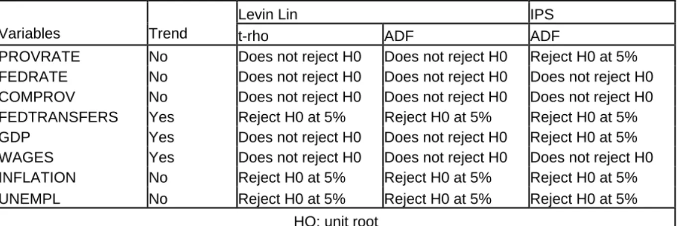
study conducted in United States where the population of States is considerably larger. We can observe results of unit root tests made with RATS in table 2.

Table 2 – Stationary Tests Results (level form)

Levin Lin IPS

Variables Trend _{t-rho ADF ADF}

PROVRATE No Does not reject H0 Does not reject H0 Reject H0 at 5%

FEDRATE No Does not reject H0 Does not reject H0 Does not reject H0

COMPROV No Does not reject H0 Does not reject H0 Does not reject H0

FEDTRANSFERS Yes Reject H0 at 5% Reject H0 at 5% Reject H0 at 5%

GDP Yes Does not reject H0 Does not reject H0 Reject H0 at 5%

WAGES Yes Does not reject H0 Does not reject H0 Does not reject H0

INFLATION No Reject H0 at 5% Reject H0 at 5% Reject H0 at 5%

UNEMPL No Reject H0 at 5% Reject H0 at 5% Reject H0 at 5%

HO: unit root

The results reported are those produced by Levin and Lin both with t-rho and Augmented Dickey-Fuller, and by Im-Pesaran-Shin (IPS) tests with the inclusion of a time dummy. If we cannot reject H0, we suppose the presence of a unit root, and thus non-stationarity. As expected, the three tax variable series are found to be non-stationary for all three tests with the exception of PROVRATE for which we reject the null hypothesis of non-stationarity for the IPS test.

WAGES and GDP are the only non-tax variable for which we cannot reject the null hypothesis for all the tests. These results come from the decision to use nominal per capita GDP and wages as the data has been shown to be stationary when indexed to inflation3.

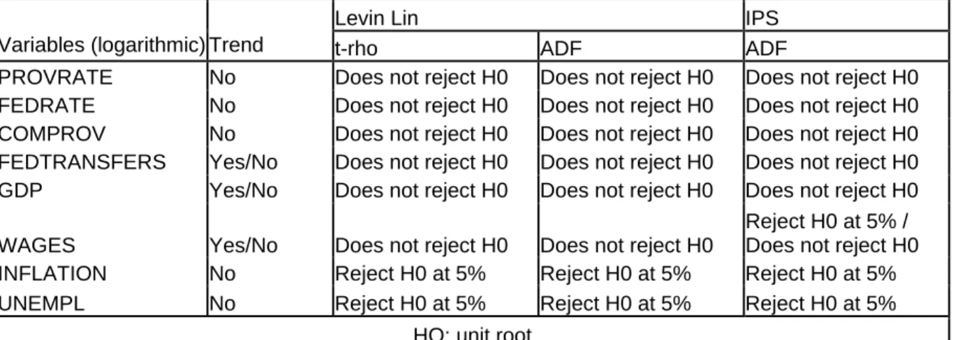
Using the logarithmic form of the variables does not help to solve the problem. As we can see in table 3, we cannot reject the null hypothesis for any variable except for INFLATION and

UNEMPL. There exist other problems related to the use of logarithmic form. In common

regressions with OLS controlled for fixed effects, variable LOGNEIGHBOUR was found to have a significant negative coefficient which would mean that a decrease in a competing province’s

tax rate would cause a province to increase its own rate. This is a very unlikely situation that is inconsistent with other results we produced (see Results section), with economic theory and with previous empirical studies, even though as a non-linear transformation logarithmic form is likely

Table 3 – Stationary Tests Results (logarithmic form)

Levin Lin IPS

Variables (logarithmic) Trend _{t-rho ADF ADF}

PROVRATE No Does not reject H0 Does not reject H0 Does not reject H0

FEDRATE No Does not reject H0 Does not reject H0 Does not reject H0

COMPROV No Does not reject H0 Does not reject H0 Does not reject H0

FEDTRANSFERS Yes/No Does not reject H0 Does not reject H0 Does not reject H0

GDP Yes/No Does not reject H0 Does not reject H0 Does not reject H0

WAGES Yes/No Does not reject H0 Does not reject H0

Reject H0 at 5% / Does not reject H0

INFLATION No Reject H0 at 5% Reject H0 at 5% Reject H0 at 5%

UNEMPL No Reject H0 at 5% Reject H0 at 5% Reject H0 at 5%

HO: unit root

to produce such results statistically. Thus, results are not reported for the logarithmic form. This leaves us two options to overcome non-stationarity in our series.

A first option we have to deal with non-stationary series is to see if those variables are

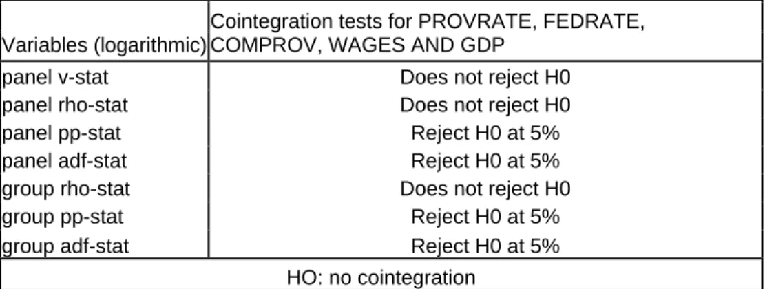
cointegrated. If they are, we can use the option of Dynamic Ordinary Least Squares (DOLS) to overcome the problem. Our series follow the same stochastic tendency which means that our estimators are convergent. RATS calculates cointegration tests using various alternative

statistics. Results are provided in table 4. The panel statistics are within-dimension based while the group statistics are between-dimension based (Morand Perreault, 2007). As we can observe, it is hard to be conclusive about the results of these tests since more conservative ones do not reject the null hypothesis of no cointegration. In a small population sample, the rejection of null hypothesis for the group rho-stat should be conclusive that we have a cointegration relation, which is not the case here (Pedroni, 2004).

Similar results are found when we try to test fewer variables for possible cointegration relations. The exception is when the tests are conducted for PROVRATE alone with FEDRATE where we can reject the null hypothesis for all seven statistics. Nevertheless, the use of estimation methods considering this relationship and including other non-stationary series in the regression would hardly be relevant for identification purposes. Even though we cannot conclude on the existence

Table 4 – Cointegration Tests Results

Variables (logarithmic)

Cointegration tests for PROVRATE, FEDRATE, COMPROV, WAGES AND GDP

panel v-stat Does not reject H0

panel rho-stat Does not reject H0

panel pp-stat Reject H0 at 5%

panel adf-stat Reject H0 at 5%

group rho-stat Does not reject H0

group pp-stat Reject H0 at 5%

group adf-stat Reject H0 at 5%

HO: no cointegration

of a cointegration relation between all non-stationary variables, results provided give us good insight into the likelihood of a cointegration relation. Thus, we provide results obtained from DOLS regression. It is risky anyway to use these since observations are lost for each lag or future value of first difference included in the regression. Because our sample is already small, we have chosen to use the first difference and one lag of it for each cointegrated independent variable. We compared the results obtained with different possible combinations of lags and advances to be sure this choice will not affect the validity of the results. We still lose 2

observations for each province with this method in addition to the one lost because of the need to use a fixed-effects model. We then drop to only 21 annual observations for each province.

The second choice we have is to use estimation methods under the first difference form. The interpretation of the coefficients will then become the impact of a variation of an independent variable (ex. FEDRATE) on the variation of the dependant variable (PROVRATE). The model then takes the following form:

Δ PROVRATE

Δ FEDRATE

Δ COMPROV

Δ FEDTRANSFERS

Δ Z

The first difference form causes the unit root parameter to disappear and thus the model becomes stationary. Nevertheless, exogenous variables significance in explaining the provincial tax rates variations is likely to be lost, which is the cost of using this form in our analysis. Even

considering this ultimate possibility, the first difference form is still likely to be our best option to deal with non-stationarity problems.

3.1.3 Heteroskedasticity, contemporaneous and serial correlation

Various tests operated in STATA helped us to specify the best estimation method considering the possible addition of heteroskedasticity, contemporaneous correlation and serial correlation

problems to our stationarity problem. In a way to identify the changes that might occur in

correcting for those problems, the tests have been made in all three forms, level, logarithmic, and first difference.

A Breush-Pagan test is used to detect heteroskedasticity. Under the null hypothesis, residual terms are homoscedastic. Should the null hypothesis be rejected, an additional test must be run to specify the form of this heteroskedasticity, to see if there is inter-individual heteroskedasticity. Such a test is operated systematically by STATA with the command “xttest2” where the rejection of the null hypothesis helps us to conclude that there is intra-individual heteroskedasticity, which does not exclude the presence of inter-individual form of heteroskedasticity. If we do not reject H0, then we can conclude that only the former is present if the null hypothesis is rejected for the first test.

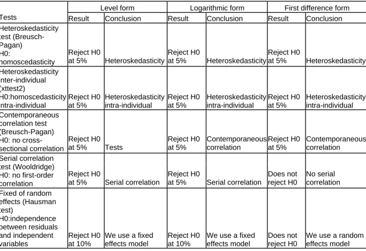
Contemporaneous correlation is detected by another Breush-Pagan test under which rejection of the null hypothesis leads us to the conclusion that there is no such correlation. The presence of serial correlation is detected by a Wooldridge test. Under the null hypothesis we can conclude that there is no first-order correlation. In table 5 are summarized all the results provided by these tests for the three forms, and results for the Hausman test to determine if we must use a fixed-effects model or a random-fixed-effects model.

We see that for the level form, all the problems mentioned are found in the data. This is useful for the DOLS method to correct those problems. With the command XTGLS, we can take into account the presence of first-order serial correlation, cross-sectional correlation and

heteroskedasticity. All these combined problems are controlled for using a Feasible Generalized Least Squares (FGLS) regression specifying the corrections we want to impose in STATA. Similar results were found for the logarithmic form for which all the null hypothesis are rejected.

Some changes in the test results occurred in the first difference transformations. We still have to deal with heteroskedasticity problems and cross-sectional correlation in data. The null hypothesis of no serial correlation in the data is no longer rejected though, so we do not have to concern ourselves with this correction in regressing first differences of our variables. Also, we do not reject the null hypothesis that residuals and explicative variables are independent. This means that both the “within” and the “between” estimators are unbiased and thus, we can use a random-effects model. Nevertheless, the presence of heteroskedasticity and contemporaneous correlation leads us to choose a GLS regression with appropriate corrections. We can note that STATA operates the same first differences regression with the OLS with random-effects model as with the GLS without additional specifications model. As only the former allow us corrective functions for heteroskedasticity and cross-sectional correlation, this estimation method is the natural choice for our concerns.

Table 5 – Tests Results Summary

Level form Logarithmic form First difference form

Tests _{Result Conclusion Result Conclusion Result Conclusion}

Heteroskedasticity test (Breusch-Pagan) H0: homoscedasticity Reject H0 at 5% Heteroskedasticity Reject H0 at 5% Heteroskedasticity Reject H0 at 5% Heteroskedasticity Heteroskedasticity inter-individual (xttest2) H0:homoscedasticity intra-individual Reject H0 at 5% Heteroskedasticity intra-individual Reject H0 at 5% Heteroskedasticity intra-individual Reject H0 at 5% Heteroskedasticity intra-individual Contemporaneous correlation test (Breusch-Pagan) H0: no cross-sectional correlation Reject H0 at 5% Tests Reject H0 at 5% Contemporaneous correlation Reject H0 at 5% Contemporaneous correlation Serial correlation test (Wooldridge) H0: no first-order correlation Reject H0 at 5% Serial correlation Reject H0 at 5% Serial correlation Does not reject H0 No serial correlation Fixed of random effects (Hausman test) H0:independence between residuals and independent variables Reject H0 at 10% We use a fixed effects model Reject H0 at 10% We use a fixed effects model Does not reject H0 We use a random effects model 3.1.4 Endogeneity

The last econometric issue we need to consider is potential problems of endogeneity for the tax variables, COMPROV and FEDRATE. The first test operated is the Nakamura-Nakamura test for endogeneity. Essentially, we regress the endogenous variable on exogenous and instrumental variables, recuperate the residuals which we include in the original regression. If the student statistic shows that the residual variable is insignificant, we reject the hypothesis of endogeneity. The second test is a classic Hausman test for validity of instruments. Under the null hypothesis, the difference in the two models, with and without instrumental variables, is not significant.

A natural instrumental variable to include in this test is a lag of the endogenous variable. This instrument is considered to be correlated with tax variables in time t and should fix the problem of correlation between the original variable and residuals of the regression. Thus, tests have been run using a lag of the federal tax rate and a lag of competing provinces’ weighted average rate. We ran additional tests using a different instrument for FEDRATE. The average effective corporate income tax rate of the federal government in all Canada was a potential candidate. As tax bases are largely similar for federal and provincial governments within a province, the general federal rate could have been a good way to evaluate federal behaviour in setting his tax rate.

Both tests described below were used on variables in their first difference form, which possibly fixes our endogeneity problem, if there is any. Results show that this is the case here. The first test was not conclusive for COMPROV as we could not reject the null hypothesis at a confidence level of 10%. The variable FEDPROV did not show evidence of endogeneity after proceeding to the Nakamura-Nakamura test using either a lagged value of the variable or the general federal tax rate in Canada. The second test was done as well on both variables to evaluate the validity of the chosen instruments. In the three cases, we clearly could not reject the null hypothesis and we then concluded that the potential instruments are not useful. The DOLS method eliminates the need for testing for endogeneity problems, consequently there is no need to run these tests in the level form for our second regression.

3.2 Data

3.2.1 Tax Variables

Businesses in Canada deal with a complex fiscal system. For instance, small businesses in Canada, by both the federal and all ten provincial governments, can count with favourable policies such as a preferential rate and other deductions. Other differentiating treatments have been given to manufacturing and processing businesses during the years covered in the present study. Depreciating methods and allowances are another example of tools governments can use

as incentives to influence corporate activities in Canada. In this respect, average effective rate are a good way to summarize all those different treatments within the country or the provinces.

Nevertheless, while capturing differentiations in the taxation regime, other realities concerning capital mobility between provinces that should be considered are not. Some provinces offer particular services or favours that give them an additional advantage in attracting firms. For instance, Quebec charges electricity rates below the general price to aluminum producing companies which impacts on some firm’s decision to invest in that province. Also, economic theory generally focuses on the marginal rate, not the average rate, to be the determinant factor in firm’s investment decisions. Devereux et Griffith (1998) argue in favour of average tax rates supposing that once firms decided to enter a foreign market, average tax rates are more important in the choice of a production location.

Average effective tax rates depend on two elements: direct taxes revenues from corporations and government enterprises, and the tax base, which are the corporate profits before taxes. Both are collected from CANSIM in provincial economic accounts. Horizontal interactions are measured by a weighted average of all nine other provinces’ rates for each province. The relative

importance of each province in the variable is exclusively determined by its proportion in the total GDP of the nine provinces. This contrasts with Karkalakos and Kotsogiannis’ (2007) geographical criterions approach but is consistent with Hayashi and Boadway’s (2001) one. We operate under the assumption that geographical considerations are not relevant for capital considering its high mobility but economic activity is. Theory is not clear on whether distance must be taken into account for investment location decisions within a federation or not.

Table 6 – Data Description and Source, 1981-2004, Canada

Variable Definition

Source

PROVRATE Provincial average effective corporate income tax rate as a proportion of direct taxes from corporations and governments business enterprises on corporate profits

Provincial economic accounts, CANSIM, Statistics Canada

Variable Definition

Source

FEDRATE Federal average effective corporate income tax rate in each province as a proportion of direct taxes from corporations and

governments business enterprises on corporate profits

Provincial economic accounts, CANSIM, Statistics Canada

NEIGHBOUR Weighted average of competing provinces’ average effective corporate income tax rate as a proportion of direct taxes from

corporations and governments business enterprises on corporate profits

Provincial economic accounts, CANSIM, Statistics Canada

FEDTRANSFERS Per capita current transfers from federal government to provinces

Provincial economic accounts, CANSIM, Statistics Canada EQUAL =1 if province receive equalization

payments in specific year

Finances of the Nation, Canadian Tax Foundation WAGES Per capita wages, salaries and

supplementary labour income

Provincial economic accounts, CANSIM, Statistics Canada GDP Per capita GDP, 1997 constant prices Provincial economic

accounts, CANSIM, Statistics Canada INFLATION Inflation rate calculated from CPI based on

a 2001 basket content, 1992=100

CANSIM, Statistics Canada

UNEMPL Official unemployment rate Labour force survey

estimates (LFS), CANSIM, Statistics Canada

In Figure 2 and 3, we observe the evolution of provincial effective rates for eastern and western provinces respectively. We note some common movements in different provincial rates that may be an indication of the presence of horizontal competition. Nevertheless, these variations can possibly be attributed to changes in corporate profits induced by the business cycle. This shows the importance of including exogenous variables to capture external effects of the business cycle

Figure 2 – Average Effective Corporate Income Tax Rate – Eastern Canadian Provinces (1981-2004)

Average Effective Corporate Incom e Tax Rate - Eastern Provinces

0,00 0,05 0,10 0,15 0,20 0,25 1981 1982 1983 1984 1985 1986 1987 1988 1989 1990 1991 1992 1993 1994 1995 1996 1997 1998 1999 2000 2001 2002 2003 2004 Ye a r Newf undland Prince- Edouar d-Island Nova Scot ia New- Br unswick Quebec

Source: Statistics Canada, CANSIM, Provincial economic accounts

Figure 3 – Average Effective Corporate Income Tax Rate – Western Canadian Provinces (1981-2004)

Average Effective Corporate Income Tax Rate - Western Provinces

0,00 0,05 0,10 0,15 0,20 0,25 1981 1982 1983 1984 1985 1986 1987 1988 1989 1990 1991 1992 1993 1994 1995 1996 1997 1998 1999 2000 2001 2002 2003 2004 Year

Average effective tax rate

Ontario Manitoba Saskatchewan Alberta British-Columbia

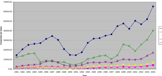
Figures 4 and 5 helps us to understand some facts about the average tax rates patterns. We should note that the values used in these figures, unlike those used to calculate average tax rates, are deflated4 for inflation in order to simplify their interpretation. Generally speaking,

movements in tax rates seem to be the opposite of those of the tax bases. In the beginning of the 1990’s, tax bases commonly shrank following a period of economic slowdown characterized by negative growth rates for most of the Canadian provinces. In contrast, a higher proportion of corporate profits was taxed by provincial governments in those years, which tends to demonstrate that governmental revenues are not affected in the same proportion as corporate profits when the economy experiences a slowdown. The opposite is also true as the following years were

characterized by growing corporate profits while average rates tended to decrease. Thus, we can reasonably conclude that the tax base is more responsive to business cycles than revenues from corporate income tax, and thus a bias could be appear if exogenous variables were omitted.

Figure 4 – Provincial Corporate Tax Base – Eastern Canadian Provinces (1981-2004)

Provincial Corporate Tax Base - Eastern Provinces

0,00 5000,00 10000,00 15000,00 20000,00 25000,00 30000,00 1981 1982 1983 1984 1985 1986 1987 1988 1989 1990 1991 1992 1993 1994 1995 1996 1997 1998 1999 2000 2001 2002 2003 2004 Year Co rp o rate tax b ase Newfundland Prince-Edouard-Island Nova Scotia New-Brunswick Quebec

Source: Statistics Canada, CANSIM, Provincial economic accounts

Figure 5 - Provincial Corporate Tax Base – Western Canadian Provinces (1981-2004)

Provincial Corporate Tax Base - Western Provinces

0,00 10000,00 20000,00 30000,00 40000,00 50000,00 60000,00 70000,00 1981 1982 1983 1984 1985 1986 1987 1988 1989 1990 1991 1992 1993 1994 1995 1996 1997 1998 1999 2000 2001 2002 2003 2004 Year Co rp o rate tax b ase Ontario Manitoba Saskatchewan Alberta British-Columbia

Source: Statistics Canada, CANSIM, Provincial economic accounts

We use federal average effective rates on corporate income tax are built the same way as provincial ones. They are based on federal government revenues from corporate tax in each province separately. The tax base is derived from corporate profits calculated identically at both the federal and provincial levels. Even though three provinces, Ontario, Quebec and Alberta, administer their own corporate tax, they use a relatively similar tax base as the federal

government. For the other seven provinces, tax bases are consistent with the federal ones.

The period considered in the present study has been characterized by a commitment of the federal government to reduce the tax burden of businesses to promote investment. The statutory rates have been decreasing constantly since 1981 for all kinds of businesses as we can observe in table 7. The general business rate decreased from 46% to 21% between 1981 and 2004, while the small business’ lower rate threshold increased from 200 000$ to 250 000$ during the same period.

The results of that policy can be observed in figure 6 where we see the federal corporate tax revenues and tax base for the whole country. The data shown does not correspond to that which Table 7 – Statutory Federal Corporate Income Tax Rates in Canada, Selected Years, 1981-2004

Federal Corporate Income Tax Rates, Selected Years, 1981 to 2004

Statutory tax rates

Type of business _{1981 1987 2003 2004}

General business 46% 36% 23% 21%

Manufacturing and processing 40% 30% 21% 21%

Natural resources N/A 36% 27% 26%

Investment income N/A 36% 28% 28%

Small business rate 25% 15% 12% 12%

Threshold 200 000$ 200 000 $ 225 000 $ 250 000 $

Source: Finances of the Nation, 1981-82 and 2005, Canadian Tax Foundation

Figure 6 – Federal Corporate Tax Revenues and Tax Base, Canada (1981-2004)

Federal Tax Revenues and Tax Base

0,00 20000,00 40000,00 60000,00 80000,00 100000,00 120000,00 140000,00 160000,00 1981 1982 1983 1984 1985 1986 1987 1988 1989 1990 1991 1992 1993 1994 1995 1996 1997 1998 1999 2000 2001 2002 2003 2004 Year F e d e ral tax reven u es an d tax b ase

Corporate tax revenues Corporate tax base

we use, namely it is not separated by province, but is relevant to evaluate the central administration behaviour globally. The same phenomenon as with provincial rates can be observed at the federal level, that the tax base is a lot more responsive to business cycle than tax revenues. It is clear also that the average effective federal rate decrease corresponds to an increase in the tax base while policies of lowering statutory rates by the government result in a very modest increase of tax revenues from corporations.

3.2.2 Other Variables

Average marginal corporate income tax rates are the common tool used to predict provincial governments’ policies since changes in those rates allow us to distinguish governments’ reactions to federal and competing provinces’ ones. Nevertheless, they are not perfect indicators of these behaviours and for this reason, we have to include other external factors that have an impact on these rates.

Provinces’ fiscal capacity is evaluated under 33 tax bases that are compared to national standards calculated by an average of five representative provinces, Ontario, Quebec, British Columbia, Saskatchewan and Manitoba. The program has been amended since, but the period we cover in this study is not concerned by the changes.

Equalization entitlements is a variable of interest because of the possible “tax-back effect”. Because revenues from equalization are affected by an eventual increase in the size of a tax base, it is suspected that equalization system might cause disincentive to reduce tax rates. We use a dummy variable to see if there is a difference in behaviours of beneficiary and non-beneficiary provinces. The decision to use a dummy instead of actual numbers was made based on two results. First, Calvolic and Day (2003) found that there is no empirical evidence of a “tax-back effect” and thus provinces do not seem to deliberately adopt policies that could negatively affect their tax bases. Second, Karkalakos and Kotsogiannis (2007) found no evidence of a

effective rates as we mentioned before. Karkalakos and Kotsogiannis (2007) assume the rates are influenced by one year retarded entitlements and thus can be treated as general federal transfers. If current transfers from federal government are such that they impact provincial rates, then we may conclude, as Karkalakos and Kotsogiannis (2007), that lagged equalization payments have a similar impact.

Federal transfers per capita, are considered relevant because they negatively affect provincial tax rates. Higher transfers increase provinces’ revenues and put downward pressure on their rates. The variable is lagged by one year as transfers should be considered as lump-sum payments that will affect governments’ positions the following year.

Other variables are expected to have an effect on average effective provincial rates. GDP per capita, inflation rate and wages per capita must be considered as indicators of the business cycle, which influence corporate profits, and are external to provincial administrations’ behaviours. Inflation is also relevant as the tax base is not indexed for inflation. The unemployment rate is considered to account for the possibility that the production factor “labour” might be

underemployed. International interest rates, captured in previous work (Hayashi and Boadway (2001), Karkalakos and Kotsigiannis (2007)) by nominal rates on U.S. municipal bonds, have been voluntarily omitted since the variable was not considered as significant in the preceding studies mentioned. We note that per capita GDP, wages and federal transfers are not indexed for inflation because nominal values of the tax base and corporate income tax revenues are used to calculate average tax rates.

3.3 Results

Running two different regressions for our model offers a good way to be more secure about our conclusions. The first difference approach calculates how changes in tax rate variations from one year to another are correlated between provinces and federal rates. While the first difference form interpretation is more difficult than with a level regression, all econometric problems

analyse since their relative magnitude and significance reveal which variables have an impact on the provincial average tax rates and the relative importance of those factors.

The DOLS method used with Feasible GLS also offer us a regression free of major econometric problems. Nevertheless, the small number of periods considered limits us in the implementation of this method. The advantage here is that the coefficients will be much easier to analyse. It directly calculates the effect of a change in federal or competing provinces’ rate on provincial ones. The most important thing is that, as it can be seen in table 8, results of such different forms of regression are consistent, and so we can conclude that these results are robust to such

transformations.

3.3.1 Vertical tax interaction

In both estimation methods, the federal tax rate is shown to have a significant positive effect on the provincial tax rate. From a theoretical point of view, this would mean that provincial

governments have more interest in preserving their revenues than their tax base, the former being the quantity of capital on their territory. When the federal government increases its rate,

provinces will tend to increase theirs to compensate the loss of revenues caused by the reduction of their tax base. If on the other hand the federal rate decreases, provinces seem to put more emphasis on maintaining government’s revenues stable than preserving the tax base. Economic theory is not clear about the sign that the coefficient should take, and according to Keen (1998), both possibilities are plausible depending on different factors.

The positive interaction found in our two regressions is inconsistent however with Karkalakos and Kotsogiannis’ (2007) and Hayashi and Boadway’s (2001) results on corporate income tax. They found a negative relation for all the provinces with the federal government in fixing tax rates. Their analyses were quite different though in various regards, including the period covered and the econometric methods. Esteller-Moré and Solé-Ollé (2001) found a positive relation between federal and provincial rates for personal income tax rates in Canada.

Table 8 – Estimation Results for PROVRATE regressions

GLS 1st difference DOLS

Variable

FEDRATE 0.3103827*** (11.14) 0.2686443*** (7.04) COMPROV 0.18628** (2.48) 0.3214822*** (3.82) EQUALIZATION 0.0006045 (0.39) 0.0068209 (1.62)

FEDTRANSFERS (1 lag value)

-0.0000121*** (-2.58) -7.26e-06** (-2.18) INFLATION 0.0378258 (0.56) 0.0005896 (0.01) WAGES 4.12e-06 (1.25) 7.93e-06*** (3.86) GDP -2.99e-06*** (-2.63) -3.70e-06*** (-3.59) UNEMPL -0.0205219 (-0.20) -.0672182 (-1.07)

Note: *, **, *** indicate statistical significance at the 0.10, 0.5, and 0.1 levels respectively Source: calculations by the author

A positive relation has important concrete implications. This would imply that the federal government may be able to partly compensate the loss in corporate income tax revenues from a decrease in its tax rate as the ensuing decrease in provincial rates would increase the size of the tax base. Also, it is very useful for the central administration to fully understand how to affect the combined rate of taxation in Canada, since it is affected by the country-wide evolution of the tax base, both for revenues and capital attraction reasons. If it has the will to encourage

achievable than if provinces were responding with a increase in their rate. This provincial increase would cancel at least partly federal efforts to reducing tax burden of businesses, and could even lead to an overall increase of the combined rates. Nevertheless, the opposite is also true. It makes it harder for federal government to increase its rate as a source of additional revenues since a subsequent increase in provincial rates minimize this gain because of the amplified negative effect on the tax base.

3.3.2 Horizontal tax interaction

Economic theory is much more defined and documented regarding horizontal tax interaction both between sub-national governmental entities and between countries. Same level administrations tend to compete between themselves in fixing their tax rate to attract capital and prevent capital to flow out of their territory. Our results are consistent with this assumption. Both regressions show positive coefficients of interaction between Canadian provinces. A decrease in another provinces’ tax rates impose downward pressure on a given provincial tax rate. What is not clear though is whether horizontal interaction influences are relatively more important than vertical ones. The first difference estimation reports a higher coefficient of reaction to a change in federal rate than competing provinces’ ones while the DOLS estimate shows the opposite. We cannot compare however the two regressions on this point because both the interpretation and the estimation method are different.

A comment concerning the preceding empirical studies mentioned before needs to be made. Unlike Karkalakos and Kotsogiannis, we have chosen not to make any assumption about a possible geographical proximity relation to construct our variable of competing provinces. Our results are still conclusive about the existence of horizontal tax interaction, so it seems that even without the geographical dimension, there is still a significant link between the provinces’ tax rates. This is an argument in favour of assuming a high mobility of capital, even though we cannot reject the existence of a geographical dimension to horizontal competition. The methods we have chosen do not allow us to identify a particular relation within a group of provinces. Hayashi and Boadway (2001), using three sub-national players with a two-way interaction model,

were able to identify a specific interaction between Ontario and Quebec for example, and so were Karkalakos and Kotsogiannis (2007) in evaluating a distinct coefficient for each province. We did not however risk disaggregating our sample to produce a coefficient for each province considering the small number of periods we use for each.

3.3.3 Federal transfers and equalization

As we said before, equalization payments are expected to affect tax rate setting in reducing the cost of increasing them. We do not find a relation such that provinces receiving equalization entitlements tend to act differently in underestimating the cost of a reduction of their tax base. Calvolic and Day (2003) arrive at similar results studying specifically the “tax-back effect”.

In the case of federal transfers, they seem to affect negatively and significantly provincial tax rates with a one period lag. Those transfers received have an impact on provincial budgets of the following year and thus put downward pressure on governments need for other forms of

revenues. Like us, Karkalakos and Kotsogiannis (2007) have found a negative relationship between federal transfers with a lag and provincial tax rates. They also found that preceding year equalization entitlements follow a similar dynamic. We do not use values of equalization

payments in our study but we can assume that, with one period lag, they have the same impact as other transfers.

This is an interesting result if we consider how the variable FEDRATE influences the provincial rates. Even though we did not study the direct relation between federal tax rate and federal transfers, we can easily consider the possibilities it brings to the federal government to pursue different goals. Depending with what magnitude transfers and federal tax rate can affect provincial ones, a combination of those two variables can be a useful tool. The loss of revenue for the federal government that results from fixing a lower tax rate could be compensated by lower transfers to provinces. The provincial rates being positively related to variations in the federal tax rate, should lead, according to our results, to a lower combined rate with a minimized

loss for the federal government. Provinces also benefit from the resulting larger tax base even if it is impossible for us to determine the net effect on their revenues.

Of all the exogenous variables used in our model, only GDP shows a significant coefficient in both regressions and WAGES with the DOLS method. The GDP has a negative impact on average effective provincial rates. This can be explained by the important relationship of this variable with the tax base of a province. The coefficient of WAGES, on the hand, shows a positive impact of this variable on PROVRATE. A likely explanation would be that corporate profits are reduced when higher wages are paid. Inflation rate and unemployment rate do not have a significant effect on provincial tax rates.

3.3.4 Horizontal and vertical externalities

In light of our results, we can assume the presence of horizontal externalities for Canadian provinces under the classic form. Because of the mobility of the tax base, the cost of public collection of additional taxes from corporate income is higher than it would be without such competition. The result of this dynamic is that all provinces are expected to set a lower tax rate than the optimal one where marginal cost of public found (MCPF) equal its marginal revenue in absence of tax competition.

Under the assumption of vertical externalities, we consider the provincial tax rate to be higher than the optimal one because it does not take into account the pressure it creates on federal revenues in reducing the tax base. If the federal government increases its rate, the provinces tend to increase their rates as well, to compensate the loss of revenues. If provincial tax rates are too high, our results show that the federal government, being able to influence positively those rates, have a tool to minimize this kind of negative externalities in decreasing its own rate which would not be the case with a negative coefficient. It is not clear which kind of pressure dominates the other, or which type of externality is the most important. However, we know that the federal government has diminished its importance in the corporate income tax field over the years, so that vertical externalities have probably decreased as well.