D
OCUMENT DE
T
RAVAIL
DT/2002/03
Can a relation be found between
inequality and growth ?
Denis COGNEAU
Charlotte GUENARD
CAN A RELATION BE FOUND BETWEEN INEQUALITY AND GROWTH 1 ? Denis Cogneau
(IRD et DIAL) Charlotte Guénard (IEP Paris et DIAL) e-mail : [email protected]
Document de travail DIAL / Unité de Recherche CIPRE Janvier 2002
RESUME
Ce travail revient sur l’économétrie de la relation entre inégalités et croissance, à l’échelle macro-économique des pays. Il s'intéresse particulièrement aux conséquences des choix de spécification, de la méthode d'estimation et de la sélection de l'échantillon. Il conclut à l'absence d'une relation robuste allant des inégalités de revenu vers la croissance du produit par tête ou vers l'investissement physique et humain. Une relation de causalité inverse, conforme à la philosophie de la courbe de Kuznets, paraît mieux assise. En tout état de cause, les stratégies de développement nationales et les configurations structurelles et historiques de chaque société conservent une place très large pour déterminer les évolutions conjointes du revenu et de sa répartition.
ABSTRACT
This work takes a new look at the econometrics of the national- level macroeconomic relationship between inequality and growth. It focuses, in particular, on the effects of specification choices, estimation method and sample selection. It concludes that there is no robust relation running from income inequality to per capita product growth or physical and human investment. There would seem to be more grounds for an inverse causal relation in keeping with the Kuznets curve philosophy. In any case, the national development strategies and structural and historical configurations of each society still play a major role in determining concurrent changes in income and its distribution.
1 Our thanks go to the participants in the DIAL-Paris I development economics seminar, and the members of the CREST Macroeconomics Lab
Content
INTRODUCTION... 4
1. THE SPECIFICATIONS... 6
2. THE ESTIMATION ... 7
3. THE DATA... 11
4. DOES INEQUALITY HAVE A NEGATIVE OR POSITIVE EFFECT ON GROWTH?... 13
5. A KALDORIAN INVESTMENT MODEL? ... 16
6. IS INEQUALITY FAVOURABLE TO EDUCATION RATES AND LOWER FERTILITY? 17 7. EGALITARIAN GROWTH?... 18
CONCLUSION... 21
REFERENCES... 22
APPENDIX ... 25
List of tables
Table n° 4-1 : Growth Equations... 14Table n° 4-1 : Banerjee and Duflo non-linear specification test ... 15
Table n° 4-2 : Non-linear specification test for the Gini index in the growth equation... 15
Table n° 5-1 : Investment equation ... 17
Table n° 6-1 : Secondary education equation ... 17
Table n° 6-2 : Fertility rate equation... 18
Table n° 7-1 : Kuznets curve estimations... 19
Table n° 7-2 : Estimations of an augmented Kuznets curve ... 20
Appendix
Appendix 1 : Dictionary of variables... 25Appendix 2 : Descriptive statistics ... 25
INTRODUCTION
Economics has long been looking at the link between distribution and production. The leading historical theories of production and allocation of resources are also theories of resource distribution and price setting (see, e.g. Schumpeter, 1954). In the 1990s, a whole host of literature appeared on this subject close on the heels of the “new” growth theories. The World Bank’s extensive international income inequality database put together by Deininger and Squire (1996) prompted a new series of econometric studies on the question. This paper is part of this series. It takes a new look at a number of stylised facts put forward by the theoretical literature. It studies, in particular, the effects of specification choices, estimation method and sample selection. It concludes that there is no robust relation running from income inequality to per capita product growth or physical and human investment and that there would appear to be more grounds for an inverse causal relation.
From the 1960s to the early 1990s, many papers were produced on this growth-to-inequality causality in the tradition of Kaldor (1956) and Kuznets (1955). For example, the Solow-based models produced by Stiglitz (1969) and then Bourguignon (1981 and 1990) discussed the conditions for finding a Kuznets curve and, more generally, the hypotheses whereby growth could create or absorb income inequality. In the 1970s and 1980s, cross-section data gathered on the developing countries appeared to corroborate the Kuznets curve (Adelman and Morris, 1973; Ahluwahlia, 1976; and Papanek and Kyn, 1986). However, it gradually became clear that the estimates were sensitive to tested functional forms and sample content (Anand and Kanbur, 1993a and 1993b). With cross-section data, however, the curve displayed a certain amount of resistance once the effect of other demographic variables, human capital and dualism, had been controlled for (Barro, 1999; Higgins and Williamson, 1999; and Bourguignon and Morrisson, 1999). Nevertheless, it did not pass the longitudinal data test as easily (Fields and Jakubson, 1994; and Li, Squire and Zou, 1998). Theoretical models continue to be based on this curve (e.g. Galor and Tsiddon, 1997; and Dahan and Tsiddon, 1998).
In the 1990s, economists turned their attention to the inverse causal relation from inequality to growth. In 1991, growth econometrics produced a new stylised fact: a negative relation between the “initial” inequality and long-run growth (Person and Tabellini, 1994; Alesina and Rodrik, 1994; Bourguignon, 1993; Birdsall, Sabbot and Ross, 1995; Clarke, 1995, Perotti, 1996; Galor and Zang, 1997). Many theoretical models were built to explain this regularity, whose robustness was taken as read for a while (see especially Clarke, 1995). Yet, as with the Kuznets curve, the “new curve” soon proved to be fragile, even on cross-section data (Fishlow, 1996; and Barro, 1999). The longitudinal analysis made by Forbes (2000) suggested a converse relation, i.e. inequality favourable to growth. Banerjee and Duflo (2000) posited that it was the variation in inequality, notwithstanding the sign, that had a negative effect on growth. The results from these two most recent papers in the series are discussed at length in section 4.
One series of theoretical models is based on a core assumption of imperfect credit markets in the financing of physical investment projects and schooling (Loury, 1981; Banerjee and Newman, 1993; Galor and Zeira, 1993; Aghion and Bolton, 1997; Piketty, 1997; and Galor and Zang, 1997). Bourguignon (1993 and 1998) and Perotti (1998) corroborated a negative link between inequality and schooling, again using cross-section data. Person and Tabellini (1994) and Perotti (1994)
posited a negative link between inequality and physical investment. However, this link was inverted by Bourguignon (1993) and invalidated by Barro (1999).
A second series of models focuses on the political economy. This was deemed especially warranted since the negative effect of inequality on growth seemed persistent despite the inclusion of physical and human investment in the econometric equations tested. The first two models were built by Person and Tabellini (1994) and Alesina and Rodrik (1994), who proposed a mechanism whereby excessive inequality induces demand for tax-distorting redistribution. This mechanism was empirically challenged by Bénabou (1996) and Perotti (1993 and 1996), who found no significant link between inequality and redistributive transfers. A less specific mechanism posited that a high level of inequality fostered political instability. Perotti (1994 and 1996) tested this correlation. Banerjee and Duflo (2000) proposed a very simple “hold-up” model in which growth opportunities are more or less efficiently exploited depending on the intensity of the distributive conflicts they create. They econometrically concluded that a non- linear relation exists between the variation in equality and subsequent growth. Last but not least, some models combine political economy mechanisms – based on different median voter variants – with credit market imperfections (Perotti, 1993; Saint-Paul and Verdier, 1993; Bourguignon and Verdier, 1997; and Lee and Roemer, 1997). These models’ findings are more complicated and have not, as yet, been corroborated empirically.
Other arguments were put forward to explain a negative link between inequality and growth. Bénabou (1994 and 1996) and Durlauf (1994 and 1996) studied local externalities and social stratification in detail. Murphy, Schleifer and Vishny (1989) proposed a new explanation based on market-size effects in the presence of growing returns on scale. The effect of inequality on fertility was also considered in an extension of the Becker, Murphy and Tamura model (1990). Perotti (1996) found a positive link between inequality and fertility, which could explain how inequality weighs on growth by slowing down the demographic transition.
The theoretical literature therefore proposes a wide variety of testable specifications and the corresponding empirical literature has obtained contrasting findings to say the least. From a strictly econometric standpoint, the techniques used until recently have been rather crude. Empirical analyses are therefore subject to two types of classic econometric biases: selection biases and endogeneity biases. This is due to the limits inherent in the available data, even in the most comprehensive base to date built by Deininger and Squire (1996). The reason for these limits is that international data on income inequality are still far from complete and vary in quality even today. This has led to radical sample selection. Analyses usually look at some fifty countries, wherein the OECD countries are over-represented. In addition, the data’s dynamic dimension is highly limited. Here again, this usually results in an unbalanced panel containing just a hundred-odd points for some forty countries from which the sub-Saharan African and poorest countries are virtually absent. The usable inter-temporal variance is also much lower than the inter- individual variance.
As regards the selection biases, some papers demonstrate that their findings are sensitive to the type of sample chosen even in the cross-section dimension. For example, Barro (1999) finds that the effect of inequality on growth varies by the level of initial income, being more negative for the poor countries and more positive for the rich countries. Since the use of the longitudinal dimension
particularities (especially in Latin America) or two levels of development (rich countries and poor countries). However, a descriptive analysis of the data suggests that the selection biases may well not be innocuous (see section 3 below). It would therefore seem preferable to keep as many countries as possible in the analyses. To do this, we have restricted the number of explanatory variables by choosing simple specifications and have introduced dummy variables for the missing data on inequality and their temporal variation.
The correction techniques for biases due to the presence of endogenous individual fixed effects are sensitive to measurement errors and favour short- and medium-run relations. These reservations led Barro (1999) to reject their use in growth econometrics. Yet the fact remains that the inter-individual dimension completely disregards the explanatory variables’ correlation with an unobserved individual effect and rules out a satisfactory test of the different theoretical assumptions. In addition to which, deviation from individual mean (“within”) estimators or first-difference estimators are inappropriate even when they are corrected for the often-large heteroskedasticity. This is because the variables’ correlation with the individual-temporal disturbance is actually highly probable. Firstly, most of the models put forward entail a codetermination of growth (or GDP level) and inequality in the form of a system of simultaneous equations. Secondly, the international database variables are subject to huge measurement errors, especially as regards the developing countries. Lastly, most of the equations’ specifications are autoregressive, starting with the growth equations, which systematically include the lagged GDP level – the convergence effect. These three problems were first tackled in growth econometrics (e.g. see Caselli, Esquivel and Lefort, 1996) with the use of instrumental variable estimators in the generalised method of moments (GMM). Arellano and Bond (1991), in particular, studied the GMM estimators for dynamic panel data models in detail and brought them into widespread use.
Although the econometric method used is important, the problems associated with model specification should not be overlooked. The above- mentioned empirical literature presents a wide variety of such problems.
The rest of this paper is hence structured as follows. The first section presents the specifications chosen for the econometric tests. The second section details the estimation techniques and the treatment of endogeneity and selection biases. A third section explains how the data were put together. Sections 4 to 7 present the findings of the econometric estimates of growth, physical investment, human investment and fertility equations, and also the Kuznets curve.
1. THE SPECIFICATIONS
We have chosen to test a set of theoretically feasible relations between inequality and growth by examining some of the channels through which this relation could subsist.
We decided first to retest the direct effect of inequality on growth, as done by most of the previous papers (Section 4). However, a growth equation still had to be chosen. The equation chosen stems from Mankiw, Romer and Weil’s specification (1992). It hence incorporates, in addition to the Gini index lagged by one period (GINI(-1)):
(i) The convergence effect in the form of the previous GDP level, LGDP(-1);
(ii) The demographic dilution effect in the form of the logarithm of the population’s annual average growth rate incremented by a 5% technological progress rate for all the countries, LGPOPC;
(iii) The effect of the logarithm of the current investment rate, LINV;
(iv) The flow of skilled manpower in the form of the logarithm of the secondary education rate lagged by two periods, SECR(-2).
We believe these last three variables to be the fundamental factors for medium-run growth. They are also each liable to be directly affected by inequality. Lastly, several non- linear specifications were tested for the Gini index using the same control variables so that we could compare our findings with Banerjee and Duflo’s results (2000).
The above- mentioned theoretical models incorporating credit market imperfections suggest a negative relation between inequality and investment, physical or human depending on the case. However, a Kaldorian model finding a positive relation between the househo ld savings ratio and household income suggests a positive relation between inequality and accumulation. We therefore endeavour to test the effect of inequality on physical and human investment. The two specifications chosen are also autoregressive. In the case of physical investment, we add in a demand-accelerator effect, which many macroeconomists consider to be one of the most robust (Section 5). In the case of human investment, we look at the primary and secondary education rate, which we associate with the per capita income level (Section 6).
In the fertility choice model, the trade-off between the number of children and their education entails the return on education and hence, indirectly, income inequality between the skilled and unskilled, as noted by Becker, Murphy and Tamura (1990). We therefore have good reason to believe that fertility depends negatively on inequality. We hence endeavour to test the impact of inequality on fertility transitions, again in an autoregressive model that adds in the per capita income level and the population’s level of education (Section 6).
Last but not least, although recent empirical literature has somewhat neglected the Kuznets curve, we present a longitudinal test of causality from growth and development variables to inequality (Section 7).
2. THE ESTIMATION
Three types of estimators are considered (see below). They are each heteroskedasticity-adjusted using the method proposed by White (1982). The variables are each expressed as a deviation from the period’s mean, which is tantamount to taking into account a temporal fixed effect considered to be certain. The unbalanced nature of the panel, which is an additional source of heteroskedasticity, is also taken into account (Arellano and Bond, 1991).
In general, the estimated models are presented as follows: v u x y yi,t =λ i,t−1+ i,tβ+ i+ i,t (1)
The ordinary least squares estimator in the total data dimension (OLS levels) provides a point of reference with the findings of previous studies on cross-section data. It largely favo urs the panel’s inter- individual dimension and provides estimates similar to those that would be found by a between estimator.
In any case, these two estimators in addition to the random effects model’s feasible generalised least squares estimator2 are unambiguously non-convergent, given the autoregressive nature of the model:
(
y, −1u)
≠0E it i (2)
Moreover, the individual fixed effect’s correlation with the other explanatory variables should not be ruled out:
(
x, u)
≠ 0E it i (3)
Hence, for the equations considered, Hausman tests comparing the fixed effects “within” estimator with the random effects feasible generalised least squares estimator systematically reject the exogeneity of the individual effect.
The ordinary least squares estimator for the first differences (OLS FD) eliminates the individual fixed effect:
(
y y)
x v y y yi,t− i,t−1= ∆ i,t=λ i,t−1− i,t−2 +∆ i,tβ+∆ i,t (4) 2This estimator is a linear combination of the between estimator and the within estimator. In our case, it would probably be “between” the “OLS levels” estimator and the “OLS FD” estimator It is the main estimator used by Banerjee and Duflo, mentioned above, to test their non-linear hypothesis (see Section 4).
This was preferred to the within estimator insomuch as it provides a point of reference for Arellano and Bond’s GMM estimator, which is an IV (instrumental variable) estimator of the first differences. The FD estimator is sensitive to three types of bias: (i) an autoregressivity bias, (ii) a simultaneity bias, and (iii) measurement error biases on the explanatory variables.
The models’ autoregressive nature immediately implies a correlation between the lagged endogenous variable and the first differences of the errors:
(
y, −1v, −1)
≠0⇒ E(
∆y, −1∆v ,)
≠0E it it it it (5a)
Furthermore, the simultaneous determination of certain variables, such as the growth rate and the investment rate, by unobserved temporal idiosyncratic elements could result in a correlation between the current values of the explanatory variables and the first differences of the errors:
(
, ,)
0(
, ,)
0(
, ,)
0 , , , ≠ ∆ ∆ ⇒ ≠ ⇒ ≠ + + = v x E v x E v E z x t i t i t i t i t i t i t i i t i t i η η α θ (5b)Lastly, the presence of additive measurement errors on the variables, which are particularly hard to avoid in the case of inequality indices, tends to bias these variables’ coefficient to zero:
(
)
(
)
( )
0 0 , * , , * , , , , * , * , , 1 , , , * , , ≤ − = ∆ ∆ ≠ − = + + + = + = − ε β β ε β λ ε t i t i t i t i t i t i t i t i t i i t i t i t i t i t i t i Var v x E v x E v v v u x y y x x (5c)The GMM(n) estimator proposed by Arellano and Bond (1991) provides a way of dealing with these three sources of bias by instrumenting the first differences of these variables using the variables’ levels lagged by 2 to (n) periods. This estimator makes the two assumptions (6a) and (6b).
The variables are first predetermined by at least one period; they are not correlated with the future residuals:
(
)
0 1 , , ≠ ≥ ∀ + v x E h h t i t i (6a)This first assumption is the most problematic, especially when variables are simultaneously determined. For example, the unobserved factors of growth in t can be correlated with the unobserved factors of inequality in t-1. For this reason, we have used lagged values of explanatory variables as much as possible.
Secondly, the error terms are not autocorrelated:
(
v, v , −1)
=0⇒ E(
∆v, ∆v, −2)
=0E it it it it (6b)
Arellano and Bond (1991) have constructed a test for this second hypothesis in the form of a second order correlation test between the first differences of the individual/temporal error terms.
Under these two hypotheses, there are good grounds for making the first differences of the variables instrumental using levels lagged by at least two periods:
(
)
(
)
0 , 2 , , , , ∆ = ∆ = ≥ ∀ − − v E y v x E h t i h t i t i h t i (7)Given that the number of orthogonality conditions corresponding to the assumptions is higher than the number of parameters to be estimated, a number of GMM estimators are possible. We therefore use a Sargan overidentification test, which is compatible with the heteroskedasticity of the error terms (see Arellano and Bond, 1991).
The effeciency of the second-stage GMM estimator was viewed with caution. Arellano and Bond’s simulation study finds a possible 20% to 30% underestimation of the coefficients’ standard deviations, for small size samples. This bias would be more pronounced in the case of heteroskedasticity. To overcome this risk of overly optimistic inference3, we have put stars by the
3
coefficients found to be significant by the first-stage estimator. We also varied the number (n) of instrument lags to test the robustness of the estimators.4
Last but not least, we endeavoured to partially handle the sample selection problem using a crude dummy variables method. We felt it too complicated to construct a Heckman-type two-stage estimator. So we simply included in the estimates the dummy variable taking the value 1 where the inequality index g is missing for period t and did the same thing for period t-1 with the first-difference estimates:
{ }
g u v x y yi,t=λ i,t−1+ i,tβ+α.Ι∃ i,t + i+ i,t (8a)(
y y)
x{ }
g{
g}
v y yi,t− i,t−1=λ i,t−1− i,t−2 +∆ i,tβ+α1Ι∃ i,t +α2Ι∃ i,t−1 +∆ i,t (8b)This dummy variables method was hence applied to a larger sample containing the missing Gini index data (Sample 1, see Section 3 below). These dummy variables are themselves instrumented using their lagged values in the GMM estimates. Estimates were also made using a smaller sample with no missing data and hence without these dummy variables (Sample 2).
3. THE DATA
Appendix 1 presents the list, abbreviations and sources of the variables used. The per capita GDP variable in international dollars and hence the growth variable (GROWTH) are taken from CEPII’s CHELEM-GDP database . The other six analytic variables are taken from the World Bank’s databases: population growth rate (GPOP) and fertility rate (FERT), primary (PRIMR) and secondary (SECR) school enrolment rates, investment rate (INV) and Gini index (GINI). This last variable is taken from Deininger and Squire’s database. We used only those inequality data deemed to be “high quality”: national coverage, clearly identified statistical source and recognised calculation method. Following econometric analysis, the Gini index was adjusted as follows: we added 6.5 points when the data were on consumer spending rather than income .
Two samples were put together. Their descriptive statistics are presented in Appendix 2. First of all, a basic panel was formed by grouping the data into seven five- year periods from 1960 to 1995. The GDP and secondary education rate levels are taken from the beginning of the period (1960, 1965, etc.). The levels of the other variables are five- year averages (1960-1964, 1965-1969, etc.).
Sample 1 was then extracted from this basic panel in such a way that it contains no missing data for the analytic variables, with the exception of the Gini index. This final sample contains 90 countries
made up of 67 developing countries and 23 developed and transition countries. For the five periods of analysis, the basic panel is non-cylinder and includes 387 points relatively well spread over time (see Appendix 2). These 387 points break down into 252 corresponding to missing data for the Gini index variation and 135 points corresponding to data that can be used to identify the effect of inequality in the first-difference estimates. These 135 points are provided by 52 of the 90 countries in the basic panel, 32 of which are developing countries and 20 of which are developed or transition countries.
We obtain Sample 2 by selecting only those countries for which we have Gini index variations for two successive five-year periods, making three successive Gini indices. This sample is reduced to 92 points and 37 countries, 21 of which are developing countries and 16 of which are developed or transition countries. This sample is very similar in size and composition to those used by authors working on the longitudinal dimension of the Deininger and Squire base (Forbes, and Banerjee and Duflo to our knowledge). For example, the samples used by Banerjee and Duflo contain 98 to 128 points and cover a maximum of 45 countries, 35 of which intersect with our Sample 2. The descriptive statistics (Appendix 2) confirm that both samples have a very similar profile. Compared with Sample 1, the poorest low-growth countries and the 1970s are barely represented. Notwithstanding the asymptotic property of the estimators, and regardless of the internal robustness tests possible, some results could be sensitive to the sample of countries and periods available. From our point of view, this sample selection by endogenous variables is a crucial problem.
We looked at this selection problem in more detail by making a multiple correspondences analysis for each of the two samples based on our growth equation specification variables expressed in first differences (see sections 2 and 3 above). The multiple correspondences analysis is probably the most suitable multivariate data descriptive analysis method for our purposes, since it makes no assumption of linear links between the variables and satisfactorily deals with the missing data. The variables are split into four categories of approximately equal size (four quartiles). This categorical data also has the advantage of being less sensitive to outliers, especially in first differences. Appendix 3 contains the charts showing the first factorial maps for each of these two analyses. These charts show solely the analysis’ active variable categories, since the bounds of the classes are explicitly indicated. For ease of chart interpretation, the country and period dummy variables are projected as additional variables, but are not reported.
The analysis’ first two axes explain a highly similar proportion of the samples’ inertia : 9% and 7.9% respectively for Sample 1 and 10.9% and 10.3% respectively for Sample 2. This first observation highlights the fact that the two clouds are rather spherical and therefore lend themselves with difficulty to the extraction of correlations; this element is expected to handicap the econometric analyses. In addition to this common point, the information structures of the two samples are quite different such as they appear on a reading of the contributions and variables’ factorial co-ordinates. This difference suggests that the corresponding growth equations will differ, especially for the Gini index effects, between the estimates with dummies for missing data (Sample 1) and the estimates on the stripped-down sample (Sample 2). It is obviously not urgent to make predictions about the econometric analysis, which is based on the “ceteris paribus” principle, unlike the descriptive analysis. Moreover, the instrumental variables methods subsequently applied are supposed to allow for a causal reading. Nevertheless, some of the regularities identified by the multiple correspondences analysis appear in the following sections.
In the case of Sample 1, the first factorial map is structured by a strong “Gutmann effect” (see Volle, 1981) associated with per capital GDP growth. The negative correlation between the contemporary rise in GDP and the growth in the previous period provides the first factorial axis. The second axis opposes the intermediate values of these two variables with the extreme values. It is important to note that this is a growth-period analysis. Each country could have experienced high and low, stable and instable growth periods over the last thirty years. Nevertheless, the OECD countries generally post moderate and relatively stable growth and therefore tend to be in the “north-east” quadrant of the graph. The developing countries group is more heterogeneous and is generally found in the centre of the first map. On average, the sub-Saharan African countries in this group are in the “west-south-west”. This position is associated with low economic growth interspersed with short- lived “booms”, low enrolment rate changes and the first phase of demographic transition. The high- growth Asian countries such as South Korea, China, Malaysia and Singapore are conversely in the “south-east”. This is due to high growth, a sharp rise in the secondary enrolment rate and, above all, sharp investment rate increases. It is interesting to note about the Gini index variation that the sharp decline category (of over two points) contributes to the formation of the first factorial map. This is associated with steady growth and a sharp rise in the education rate. Nevertheless, the other Gini index variation categories are not found at regular intervals along this first axis. This is due to the other extreme modality (increase of over 2 points), which tends firmly towards the centre of the graph and the “south-east” quadrant (high- growth Asian countries). Similarly, the missing data generally fit the average profile, even if they are more associated with the “south-west” quadrant like the sub-Saharan African countries. At the end of day, if a causal relation from inequality to growth exists, Sample 1’s descriptive analysis suggests that it would be negative, a downturn in inequality being associated with higher growth. However, it would also be dissymmetrical, since a drop in inequality is more favourable to growth than an increase is damaging to growth. This assumption is tested in Section 4.
The structure of Sample 2’s correlations is quite different. Here, the Gini index variations do not appear to be associated with any particular growth profile. However, there is a close link between an increase in the secondary education rate and a decrease in inequality, which is already notable in Sample 1. This causality is tested in sections 6 and 7.
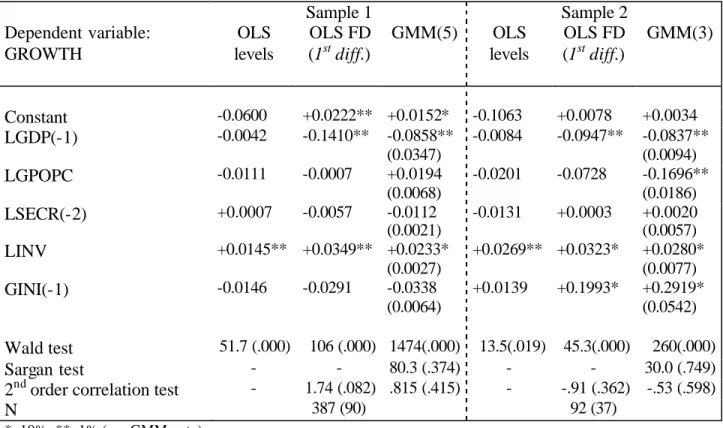
4. DOES INEQUALITY HAVE A NEGATIVE OR POSITIVE EFFECT ON GROWTH? Contrary to most of the previous findings on the effect of inequality on growth using other databases, the causal link appears to be positive for Sample 2 in keeping Forbes (2000). This link is in first differences and not in level, and it is strengthened by the instrumental variable procedure. The rough estimate of the effect is quite considerable: one additional Gini index point generates an average 0.20 to 0.3 points of additional per capita product growth. Replacing the Gini index with its logarithm results in the same type of finding. An intertemporal standard deviation variation (equal to 3.0) therefore pushes up growth by 0.6 to 0.9 points in the following period, other things being equal. Yet this finding should still be regarded with caution. It could be due to an omitted variable such as a terms-of-trade variable, which would simultaneously affect national income and its distribution. However, the introduction of the GDP price level in international dollars to reflect the real exchange rate was ineffectual. Likewise, the rate of inflation did not appear to be an explanatory factor in growth performance.
Table n° 4-1 : Growth Equations Sample 1 Sample 2 Dependent variable: GROWTH OLS levels OLS FD (1st diff.) GMM(5) OLS levels OLS FD (1st diff.) GMM(3) Constant -0.0600 +0.0222** +0.0152* -0.1063 +0.0078 +0.0034 LGDP(-1) -0.0042 -0.1410** -0.0858** (0.0347) -0.0084 -0.0947** -0.0837** (0.0094) LGPOPC -0.0111 -0.0007 +0.0194 (0.0068) -0.0201 -0.0728 -0.1696** (0.0186) LSECR(-2) +0.0007 -0.0057 -0.0112 (0.0021) -0.0131 +0.0003 +0.0020 (0.0057) LINV +0.0145** +0.0349** +0.0233* (0.0027) +0.0269** +0.0323* +0.0280* (0.0077) GINI(-1) -0.0146 -0.0291 -0.0338 (0.0064) +0.0139 +0.1993* +0.2919* (0.0542) Wald test 51.7 (.000) 106 (.000) 1474(.000) 13.5(.019) 45.3(.000) 260(.000) Sargan test - - 80.3 (.374) - - 30.0 (.749)
2nd order correlation test - 1.74 (.082) .815 (.415) - -.91 (.362) -.53 (.598)
N 387 (90) 92 (37)
*: 10%; **: 1% (see GMM note)
Estimators and tests robust to heteroskedasticity.
Dummy variables for periods (samples 1 and 2) and missing data for the Gini index (Sample 1) included, but not reported.
GMM(n): First differences instrumented by the variables’ levels lagged by 2 to (n) periods.The stars stand for the significance of the first-stage estimators. The second-stage standard deviations are potentially underestimated at a finite distance, as shown by Arellano and Bond in their simulation study. The second-stage standard deviations are given in brackets.
Table n° 0-1 : Banerjee and Duflo non-linear specification test Dependent variable: GROWTH OLS FD (1st diff.) GINI(-1) +0.3764 (0.3429) +0.2710* (0.1128) +0.2689* (0.1122) GINI(-1)² -0.2224 (0.4173) GINI(-1)-GINI(-2) +0.0901 (0.0680) +0.0899 (0.0680) -0.0667 (0.0835) (GINI(-1)-GINI(-2))² -0.0631 (1.6723) +0.0802 (1.6091) (GINI(-1)-GINI(-2))* (GINI(-1)-GINI(-2))>0 +0.0524 (0.1311) -0.0370 (0.1414) (GINI(-1)-GINI(-2))* (GINI(-1)-GINI(-2))<0 +0.1266 (0.1266) -0.0952 (0.1305) N 92 (37) *: 10%; **: 1% (See GMM note)
Estimators and tests robust to heteroskedasticity
Control variables identical to those in Table 4-1: LGDP(-1), LSECR(-2), LINV and LGPOPC, not reported. Period dummy variables included but not reported.
GMM(n): see Table 4-1 note.
Table n° 4-2 : Non-linear specification test for the Gini index in the growth equation Dependent variable: GROWTH GMM (5) GINI(-1) -0.6041 (0.0824) -0.0413 (0.0073) -0.6165 (0.0917) GINI(-1)² +0.6610 (0.0958) +0.6686 (0.1105) GINI(-1)* (GINI(-1)-0.457)>0 +0.0598 (0.0127) GINI(-1)* (GINI(-1)-0.457)<0 -0.0474 (0.0085) GINI(-1)-GINI(-2) -0.0026 (0.0266) +0.0434 (0.0261) +0.0300 (0.0294) (GINI(-1)-GINI(-2))² +1.6486 (0.6212) +1.4999 (0.7211) +1.9868 (0.8148) N 387 (90) *: 10%; **: 1% (see GMM note)
Estimators and tests robust to heteroskedasticity
Control variables identical to those in table 4-1: LGDP(-1), LSECR(-2), LINV and LGPOPC, not reported.
Dummy variables for periods (samples 1 and 2) and missing data for the Gini index (Sample 1) included, but not reported.
GMM(n): See the table 4 -1 note. The set of instruments used in this case includes solely the Gini index levels lagged by two to five periods and the levels lagged by the missing data dummy variable. No quadratic or truncated term is included, nor is any first -difference term..
But the result could also be due to the specific nature of the sample. The causality sign is indeed inversed in the case of Sample 1: inequality appears to undermine growth (left half of Table 4-1). Here, the parameter is only significant in the case of the second-stage GMM estimator. Now we have already mentioned the optimistic inference risk associated with this estimator, as shown by Arellano and Bond’s simulations. The growth equation is also of poor quality and the effects of the secondary school enrolment rate and the population growth rate have different signs to those expected. This difference between the two samples was foreseeable from the multiple correspondences analyses covered in the previous section.
Banerjee and Duflo challenge Forbes’ finding on the basis of other arguments. They posit that the Gini index variations have a non- linear effect. We decided to test the ir specification starting with Sample 2, which is very similar to theirs. The number of lags and the small size of the sample prevented us from using the Arellano and Bond estimator. We therefore made do with the first-difference ordinary least squares estimator. This estimator rejects the significance of the non- linear specifications and upholds Forbes’ finding (Table 4-2). A GMM instrumental variable procedure can be used for Sample 1. None of the Banerjee and Duflo specifications passes the significance tests. However, a non-linear effect of the Gini index level is accepted (Table 4-3). This ties up with the findings of the multiple correspondences analysis for Sample 1. This quadratic specification is significant at the 15% level using the first-stage estimator’s standard deviations. It suggests that inequality would undermine growth only up to a certain Gini index level estimated at approximately 0.457. Note that this causality is not upheld for Sample 2, in first differences (Table 4-2, first column).
5. A KALDORIAN INVESTMENT MODEL?
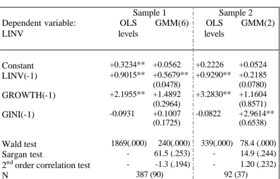
As with growth in the reduced sample, the data’s temporal dimension suggest that inequality has a positive effect on physical capital investment. This finding contradicts the imperfect credit market models mentioned in the introduction. However, it is consistent with a Kaldorian investment model based on savings rate differentials between capital and earned income and on a household savings rate that grows with income. Here again, the biases corrected by the GMM estimator appear to be highly substantial and apply to all the variables. This estimator produces a reasonable estimate of the investment rate’s hysteresis and greatly moderates the extent of the demand-accelerator effect while increasing the effect of inequality. The extent of this latter effect is nonetheless modest since, as shown by the coefficient in the last right-hand column in Table 5-1, a variation of one intertemporal standard deviation in the Gini index brings about, other things being equal, a 9% increase in the investment rate.
Moreover, this effect disappears completely when the estimate is made for Sample 1, even though the Gini index’s coefficient remains positive. The tests are hence favourable to the Kaldorian model, but do not compellingly corroborate it.
Table n° 5-1 : Investment equation Sample 1 Sample 2 Dependent variable: LINV OLS levels GMM(6) OLS levels GMM(2) Constant +0.3234** +0.0562 +0.2226 +0.0524 LINV(-1) +0.9015** +0.5679** (0.0478) +0.9290** +0.2185 (0.0780) GROWTH(-1) +2.1955** +1.4892 (0.2964) +3.2830** +1.1604 (0.8571) GINI(-1) -0.0931 +0.1007 (0.1725) -0.0822 +2.9614** (0.6538) Wald test 1869(.000) 240(.000) 339(.000) 78.4 (.000) Sargan test - 61.5 (.253) - 14.9 (.244)
2nd order correlation test - -1.3 (.194) - 1.20 (.232)
N 387 (90) 92 (37)
*: 10%; **: 1% (see GMM note)
Estimators and tests robust to heteroskedasticity
Dummy variables for periods (samples 1 and 2) and missing data for the Gini index (Sample 1) included, but not reported. GMM(n): see Table4-1 note.
6. IS INEQUALITY FAVOURABLE TO EDUCATION RATES AND LOWER FERTILITY?
In the case of the education rate, Table 6-1’s results also contradict the credit imperfection models. Yet these models were thought to be particularly predisposed to finding a negative relation between inequality and human investment, which is subject to high fixed costs and high information asymmetries. Hence in the cross-sectional dimension, inequality does effectively seem to be nega tively correlated with education rates: for an equal level of per capita GDP, the most unegalitarian countries are those where the secondary education rate is the lowest. This conditional correlation is not borne out as regards the primary education rate.
Table n° 6-1 : Secondary education equation
Sample 1 Sample 2 Dependent variable: LSECR OLS levels GMM(6) OLS levels GMM(6) Constant +2.3823** +0.0441 +1.4214* -0.0290 LPRIMR(-1) +0.8894** +0.4683** (0.0486) +1.0356** +0.2860 (0.1118) LGDP(-1) +0.4256** +0.5777* (0.0588) +0.2800** +0.6442** (0.2091) GINI(-1) -1.1410** +0.6516 (0.1255) -1.9043** +1.2734 (0.6611) Wald test 1197(.000) 854(.000) 192 (.000) 52.7(.000) Sargan test - 49.5(.684) - 13.1 (.364)
2nd order correlation test - .347 (.728) - -.95(.343)
N 387 (90) 92 (37)
*: 10%; **: 1% (see GMM note)
Estimators and tests robust to heteroskedasticity
Conversely, in the longitudinal dimension, the GMM estimators find that income inequality has a significant positive effect on the education rate. Here again, they are rather in keeping with a Kaldorian savings ratio model. Yet the estimated effect is nonetheless small at 1.5% to 6% growth in the education rate for a Gini index variation of one intertemporal standard deviation (3 points). Moreover, this effect becomes insignificant in Sample 1 when the first-stage standard deviation of the coefficient is used. Note again that the GMM estimator greatly adjusts the hysteresis effect and the GDP effect in these aggregate equations. In our estimates, income level appears to best explain the education rate rather than vice versa (see Bils and Klenow, 1998). Similar estimates were made for the primary education rate. In each case, the effect of inequality was positive, but not significant. Table n° 6-2 : Fertility rate equation
Sample 1 Sample 2 Dependent variable: LFERT OLS levels GMM(6) OLS levels GMM(2) Constant +0.2864** -0.0672 +0.2196 -0.0166 LFERT(-1) +0.9202** +0.8298** (0.0165) +0.9618** +0.9181** (0.0759) LGDP(-1) -0.0036 +0.1311* (0.0144) +0.0324 +0.0226 (0.1112) LSECR(-2) -0.0638** +0.0321 (0.0073) -0.0108 -0.0741 (0.0414) GINI(-1) -0.1928* -0.2940 (0.0296) -0.1499 -0.4224 (0.4358) Wald test 13371(.00) 5758(.000) 1043(.000) 1314(.000) Sargan test - 80.4(.164) - 19.5 (.242)
2nd order correlation test - 0.07 (.948) - 0.16 (.876)
N 387 (90) 92 (37)
*: 10%; **: 1% (see GMM note) Estimators and tests robust to heteroskedasticity. Dummy variables for periods (samples 1 and 2) and missing data for the Gini index (Sample 1) included, but not reported.
GMM(n): see Table 4-1 note.
To wind up, Table 6-2 presents an equation for the fertility rate. The same estimates were made for the population growth variable used in the growth equation (LGPOPC) and provided qualitatively similar results. The fertility rate shows the greatest inertia as shown by the GMM coefficient of the hysteresis effect, which is equal to 0.83 for Sample 1. The results for the other variables are fairly disappointing since they are not very robust. The income inequality sign is quite surprising compared with previous findings by Perotti (1996). Nevertheless, the coefficient is very small and generally not significant.
7. EGALITARIAN GROWTH?
We end this presentation of our findings with a look at an inverse causal relation from growth and human development variables to income inequality. A specific selection bias adjustment procedure should have been designed to handle the case of the missing data from the inequality variable, now become the variable to be explained. It does not matter whether the type of estimator used is “Heckman” parametric (1976) or semi-parametric as used by Lewbel (2000). The problem derives mainly from the choice of the identifying variable used in the selection equation (explaining the
absence of Gini index data), but not used in the equation explaining inequality. Since no available variable impressed itself on us, we decided to work solely with Sample 2.
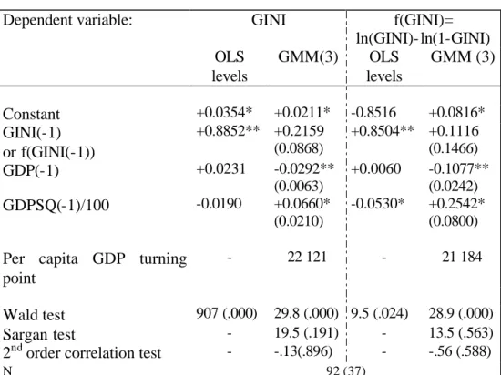
The first theoretical foundation of inverse causality is the Kuznets curve (1955). In the cross-sectional regressions, the introduced hysteresis effect quashes the significance of the quadratic effect of per capita GDP even when the sign of the coefficients confirms the inverse U-shaped form (Table 7).
However, the data’s temporal dimension only corroborates the second part of the Kuznets curve, i.e. a drop in inequality when there is economic growth. This finding is consistent with the results obtained by Fields and Jakubson (1994) from another sample using a within estimator. Since the Gini index is bounded between 0 and 1, we checked the robustness of the result by carrying out the same estimation on a transformation of this variable (right side of Table 6). At the sample’s mean point, the parabolic coefficients are identical and the turning point is very similar. All of the estimates introduce a temporal fixed effect such that the per capita GDP variable does not have to be “detrended”. The estimated curve moves by a constant value along the abscissa axis with the world growth trend.
Table n° 7-1 : Kuznets curve estimations
Dependent variable: GINI f(GINI)=
ln(GINI)- ln(1-GINI) OLS levels GMM(3) OLS levels GMM (3) Constant +0.0354* +0.0211* -0.8516 +0.0816* GINI(-1) or f(GINI(-1)) +0.8852** +0.2159 (0.0868) +0.8504** +0.1116 (0.1466) GDP(-1) +0.0231 -0.0292** (0.0063) +0.0060 -0.1077** (0.0242) GDPSQ(-1)/100 -0.0190 +0.0660* (0.0210) -0.0530* +0.2542* (0.0800)
Per capita GDP turning point
- 22 121 - 21 184
Wald test 907 (.000) 29.8 (.000) 9.5 (.024) 28.9 (.000)
Sargan test - 19.5 (.191) - 13.5 (.563)
2nd order correlation test - -.13(.896) - -.56 (.588)
N 92 (37)
*: 10%; **: 1% (see GMM note) Estimators and tests robust to heteroskedasticity Period dummy variables included, but not reported.
GMM(n): see Table 4-1 note.
The estimates even suggest the existence of a half U-shaped curve (“non- inversed”) with the parabolic turning point at the end of the sample, i.e. around the level of American per capita GDP in the early 1990s. The absence of very poor countries from the sample could explain why the riser of the real Kuznets inverse-U-shaped curve cannot be identified. So there is no reason why inequality could not operate on long cycles interspersed with technological revolutions much like the Kondratieff cycles. Although the variables’ temporal differentiation encourages medium-run relations, the GMM estimators reject the significance of the hysteresis effect to the extent that the
the sample’s mean point ($9,000 per capita, see Appendix 2), a 10% increase in GDP reduces the Gini index by 0.2 points. And as already mentioned, elasticity at the sample’s extreme point (United States) is zero.
Lastly, another model that would find the variation in inequality to be specific to each country might be more in keeping with Kuznets’ 1955 paper on English and German data. Likewise, past data confirm the steady decrease in inequality in Italy since the end of the 19th century (Rossi, Toniolo and Vecchi, 1999). Anand and Kanbur (1993a) envisage this hypothesis. We obviously cannot test such a model here since the number of observations per country is too low. In any case, the question of the interpretation of the causal relation found remains.
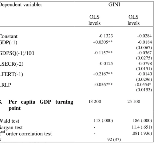
We endeavoured to make some headway with this by adding to the simple Kuznets curve the secondary school enrolment rate, the fertility rate and the Bourguignon and Morrisson dualism indicator (1999), i.e. the labour productivity relation between agriculture and the other sectors (Table 8). As found by Higgins and Williamson (1999), the Kuznets curve’s inverse U shape clearly reappears in the augmented cross-sectional regressions containing fertility. This last variable is also closely correlated with the Gini index for interindividual variance, with a correlation coefficient of over 0.6 as shown by the coefficient of the level equation minus the hysteresis effect.
Table n° 7-2 : Estimations of an augmented Kuznets curve
Dependent variable: GINI
OLS levels OLS levels Constant -0.1323 +0.0284 GDP(-1) +0.0305** -0.0184 (0.0067) GDPSQ(-1)/100 -0.1157** +0.0367 (0.0275) LSECR(-2) -0.0125 -0.0798 (0.0151) LFERT(-1) +0.2167** -0.0140 (0.0296) LRLP +0.0567** +0.0554* (0.0153)
8. Per capita GDP turning point
13 200 25 100
Wald test 113 (.000) 186 (.000)
Sargan test - 11.4 (.651)
2nd order correlation test - .081 (.936)
N 92 (37)
*: 10%; **: 1% (see GMM note)
Estimators and tests robust to heteroskedasticity
Dummy variables for periods and missing data for the dualism indicator (LRLP) included, but not reported. GMM(n): see Table 4-1 note.
The significance of per capita GDP and fertility disappears in the longitudinal data dimension, whereas the effect of the dualism variable remains despite the sampling, which eliminates a large
number of countries specialised in agriculture. The secondary education rate coefficient is
re-estimated way up compared with the cross-sectional regressions. The size of these two effects is not inconsiderable. A 10% decrease in “agricultural dualism” triggers, other things being equal, a half-point drop in the Gini index. A 10% rise in the education rate brings about a decrease in the Gini index of nearly one point. At macroeconomic level, government policies to develop education for all probably help reduce income inequality and monetary poverty. Yet even though there is no doubt that growth is “good for the poor” (Dollar and Kraay, 2000), it is probably not enough. At best, it reduces inequality slightly (see Table 6-2 comments) and degressively with the development process.
CONCLUSION
Readers will probably get an overriding impression of confusion from this paper. As concluded by Hoff and Stiglitz (1999) about economic development theory, at least the Socratic certitude of our ignorance is ascertained. However, this “informed ignorance” does not create widespread scepticism. In actual fact, avenues of research quite clearly emerge.
As mentioned in the introduction, recent theoretical literature has focused on studying the concomitant determination of most of the fundamental development variables: income level, physical and human investment, demography, and the distribution of income and resources.
The available empirical data do not reject the general idea of codetermination. Nevertheless, the econometric tests do not corroborate the decisive influence of income inequality on the other variables. Sample selection, relatively neglected by previous empirical work, proves to have problematic consequences in this regard.
It seems slightly more certain that the development process as a whole fosters a reduction in income inequality. However, it is not yet possible to separate out the different channels via which this causality occurs at macroeconomic level – demographic transition, human and institutional development, growth, etc. Here again, the question of the universality of this relation remains open due to the samples selection.
The way things stand in this field at the moment, it has to be said that the macroeconomic data work has reached its limits. Firstly, data quality continues to be a problem. All survey statisticians know the extent to which inequality index calculations are sensitive to the basic data and estimation methods. However, national accountants and social data experts are also aware of the uncertainties surrounding the more classic data on growth and other socio-economic development variables. Secondly, particular care should be taken with the estimates based on cross-section data due to their possible specification errors and bias problems. This said, a reasoned longitudinal data analysis is also limited by data quality and selection despite its challenging most of the findings obtained by the cross-section analysis. Last but not least, whatever “planetary regularities” may be discovered, they would still be surpassed by countless local particularities. The inequality- growth relation is still conditioned by national development strategies and each society’s structural and historical configurations.
REFERENCES
Adelman I., Morris C.T. (1973), “Economic Growth and Social Equity in Developing Countries”, Stanford University Press, California.
Aghion P., Bolton P. (1997), “A Theory of Trickle-Down Growth and Development”, Review of Economic Studies, 64, 151-172.
Ahluwalia M. (1976), “Inequality, Poverty and Development”, Journal of Development Economics, 6, 307-342.
Alesina A., Rodrik D. (1994), “Distributive Politics and Economic Growth”, The Quaterly Journal of Economics, 104, 465-490.
Anand S., Kanbur S.M.R. (1993a), “The Kuznets Process and the Inequality-Development Relationship”, Journal of Development Economics, 40, 25-40.
Anand S., Kanbur S.M.R. (1993b), “Inequality and development, A critique”, Journal of Development Economics, 41, 25-40.
Arellano M., Bond S. (1991), “Some Tests of Specification for Panel Data : Monte Carlo Evidence and an Application to Employment Equations”, Review of Economic Studies, 58, 277-297.
Arellano M., Bond S. (1998), Dynamic Panel Data Estimation Using DPD98 for Gauss : A Guide for Users, mimeo, 27 pp.
Banerjee A.V., Newman A.F. (1991), “Risk-bearing and the Theory of Income Distribution”, Review of Economic Studies, 58, 211-235.
Banerjee A.V., Newman A.F. (1993), “Occupational Choice and the Process of Development”, Journal of Political Economy, 101, 274-299.
Banerjee A.V., Duflo E. (2000), “Inequality and Growth: What Can the Data Say?”, NBER WP 7793.
Barro R. (1999), “Inequality, growth and investment”, NBER WP 7038.
Barro R.J., Lee J.W. (1993), “International Comparisons of Educational Attainment”, Journal of Monetary Economics, 32, 363-394.
Becker G.S., Murphy K.M., Tamura R. (1990), “Human capital, Fertility and Economic Growth”, Journal of Political Economy, 98, n°5, 12-37.
Bénabou R. (1994), “Human capital, inequality and growth : a local perspective”, European Economic Review, 38, 817-826.
Bénabou R. (1996), “Inequality and Growth”, NBER WP 5658. Benzécri J.-P. (1973), L'analyse de données, t.1 et t.2, Dunod, Paris
Bils M., P. J. Klenow (1998), “Does Schooling Cause Growth or the Other Way Around ?” NBER Working Paper 6393, 41 pp.
Birdsall N., Ross D., Sabot R. (1995), “Inequality and Growth Reconsidered: Lessons From East Asia”, The World Bank Economic Review, 9(3), 347-508.
Bourguignon F. (1981), “Pareto Superiority of Unegalitarian Equilibria in Stiglitz’ Model of Wealth Distribution with Convex Saving Function”, Econometrica, 49(6), 1469-1475
Bourguigno n F. (1990), “Growth and inequality in the dual model of development : the role of demand factors”, Review of Economic Studies, 57, 215-228.
Bourguignon F. (1993), « Croissance, distribution et ressources humaines: comparaison internationale et spécificités régionales », Revue d'économie du développement, 4, 3-35.
Bourguignon F. (1996), “Equity and Economic Growth: Permanent questions and changing answers?”, Document de travail DELTA-EHESS n°96/15, August.
Bourguignon F. (1998), « Equité et croissance écono mique : une nouvelle analyse ? », Revue Française d’Economie, 3, 25-84.
Bourguignon F., Morrisson C. (1990), “Income distribution, Development and Foreign Trade: a Cross-Sectional Analysis”, European Economic Review, 34, 1113-1132.
Bourguignon F., Morrisson C. (1998), “Inequality and Development: The Role of Dualism”, Journal of Development Economics, 57(2), 233-258.
Bourguignon F., Verdier T. (2000), “Oligarchy, Democraty, Inequality and Growth”, Journal of Development Economics, 62(2), 285-314
Caselli F., Esquivel G., Lefort F. (1996), “Reopening the Convergence Debate : A New Look at Cross-Country Growth Empirics”, Journal of Economic Growth, 1, 363-389.
Clarke G.R.G. (1995), “More Evidence On Income Distribution and Growth”, Journal of Development Economics, 47(2), 403-427.
Dahan M., D. Tsiddon (1998), “Demographic Transition, Income Distribution, and Economic Growth”, Journal of Economic Growth, 3(1), 29-52
Deininger K., Squire L. (1996), “A New Data Set Measuring Income Inequality”, The World Bank Economic Review, 10(3), 565-591.
Deininger K., Squire L. (1998), “New Ways of Looking at Old Issues: Inequality and Growth”, Journal of Development Economics, 57, 259-287.
Dollar D., Kraay A. (2000), Growth Is Good for the Poor, mimeo, The World Bank, 43 pp.
Durlauf S.N. (1996), “A theory of persistent inequality”, Journal of Economic Growth, 1(1), 75-93. Durlauf S.N. (1994), “Spillovers, stratification and inequality”, European Economic Review, 38, 836-845
Fields G.S., Jakubson (1994), “New evidence on the Kuznets Curve”, Cornell University Working Paper, mimeo.
Fishlow A. (1996), “Inequality, Poverty and Growth: Where Do We Stand?, in Bruno M., B. Pleskovic (eds)”, Annual World Bank.Conference on Development Economics 1995, The World Bank.
Forbes K.J. (1999), “A Reassessment of the Relationship Between Inequality and Growth”, MIT Working Paper, mimeo, 26 pp.
Galor O., Tsiddon D. (1997), “The Distribution of Human Capital and Economic Growth”, Journal of Economic Growth, 2(1), 93-124
Galor O., Zeira J. (1993), “Income distribution and macroeconomics”, Review of Economic Studies, 60, 35-52.
Galor O., Zang H. (1997), “Fertility, income distribution, and economic growth: Theory and cross country evidence”, Japan and the World Economy, 9(1997), 197-229.
Heckman J. (1979), Sample Selection Bias as a Specification Error, Econometrica, 47, 153-161. Higgins M., Williamson J.G. (1999), “Explaining Inequality the World Around : Cohort Size, Kuznets Curves and Openness”, mimeo, 44 pp.
Hoff K., J. Stiglitz (1999), Modern Economic Theory and Development, mimeo, The World Bank, november, 70 pp.
Kaldor N. (1956), “Alternative Theories of Distribution”, Review of Economic Studies, 23(2), 94-100.
Kuznets S. (1955), “Economic Growth and Income Inequality”, American Economic Review, 45(1), 1-28.
Lee W., J. Roemer (1997), “Income Distribution, Redistributive Politics and Economic Growth”, Journal of Economic Growth, 3(3), 217-240
Lewbel A. (2000), “Two Stage Least Squares Estimation of Endogeneous Sample Selection Threshold, or Censoring Model”, mimeo, Boston College, 32 pp.
Inequality”, Economic Journal, 108, 26-43.
Loury G. (1981), Intergenerational Transfers and the Distribution of Earnings, Econometrica, 49, 843-867
Mankiw N.G., Romer D., Weil D.N. (1992), “A contribution to the empirics of economic growth”, Quarterly Journal of Economics, 107(2), 407-437
Murphy K.M., Shleifer A., Vishny R. (1989), “Income Distribution, Market Size and Industrialization”, Quarterly Journal of Economics, 104, 537-564.
Pananek G., Kyn O. (1986), “The effect on income distribution of development, the growth rate and economic strategy”, Journal of Development Economics, 23, 55-65.
Perotti R. (1993), “Political equilibrium, income distribution and growth”, Review of Economics Studies, 60, 755-776.
Perotti R. (1994), “Income Distribution and Investment”, European Economic Review, 38, 827-835. Perotti R. (1996), “Growth, Income Distribution and Democracy: What the Data Say”, Journal of Economic Growth, 1(1), 149-187.
Persson T., Tabellini G. (1994), “Is Inequality Harmful for Growth?”, The American Economic Review, 84(3), 600-620.
Piketty T. (1997), “The Dynamics of Wealth Distribution and the Interest Rate with Credit Rationing”, Review of Economics Studies, 64, 173-189.
Popper K. R. (1959), La logique de la découverte scientifique, Payot, Paris, trad. fr. 1973
Rossi N., G. Toniolo, G. Vecchi (1999), “Is the Kuznets Curve Still Alive ? Evidence from Italy’s Household Budgets, 1881-1961”, CEPR Discussion Paper N°2140, 57 pp.
Saint-Paul G., Verdier T. (1993), “Education, democracy and growth”, Journal of Development Economics, 42, 399-407.
Stiglitz J. (1969), Distribution of Income and Wealth Among Individuals, Econometrica,.37(3), 382-397.
Schumpeter J. A. (1954), Histoire de l'analyse économique, tome III, Gallimard, Paris, trad. fr. 1983.
Volle M. (1981), L'analyse des données, Economica, Paris.
White H. (1982), Instrumental Variables Regression with Independent Observations, Econometrica, 50, 483-499.
APPENDIX
Appendix 1 : Dictionary of variables
Variable Definition Source
GDP(-1) Per capita GDP in international dollars at the beginning of the period (e.g. 1980 value for 1980-1984)
CEPII CHELEM-GDP database (1998)
GDPSQ(-1) GDP(-1) squared idem
LGDP(-1) Logarithm of GDP(-1) idem
GROWTH GDP growth rate over the period =LGDP-LGDP(-1)
idem
GINI Gini index Deininger and Squire
(1996)
[L]SECR(-2) [Log of the] Gross secondary education rate at the beginning of the period, lagged once (e.g. 1975 value for 1980-1984)
World Development Indicators (2000)
[L]PRIMR [Log of the] Gross primary education rate idem [L]FERT [Log of the] Fertility rate idem [L]GPOPC [Log of the] population growth rate +0.05 idem [L]INV [Log of the] Investment rate idem [L]RLP [Log of the] Labour productivity ratio between the agricultural
sector and other sectors
Appendix 1 : Descriptive statistics
Echantillon n°1 Echantillon n°2 A. Number of periods 1970-1974 77 9 1975-1979 81 10 1980-1984 82 20 1985-1989 78 27 1990-1994 69 26 Total 387 92 B. Means
Per capita GDP in 1985 international dollars 5185.6 9020.2
Per capita GDP growth rate (%) 1.4 2.2
Gini index 0.415 0.377
Values missing from the Gini index (%) 45.2 0.0
Investment rate (%) 17.2 22.1
Gross secondary education rate (%) 45.0 67.4 Gross primary education rate (%) 89.5 100.7
Population growth rate (%) 1.9 1.2
Fertility rate 4.3 2.6
-
- C. Number of countries per region
- Sub-Saharan Africa 29 1
- Latin America and the Caribbean 18 8
- South and East Asia 12 10
- OECD countries 19 13
Appendix 2 : Multiple correspondences analysis
Multiple correspondences analysis Sample 1
387 countries-periods, first differences of variables (D) contributions to axis 1, | contributions to axis 2 |
-1,5 - 1 -0,5 0 0,5 1 -1,5 - 1 -0,5 0 0,5 1 1,5 2 Axis 1 (inertia : 9,0%)
Axis 2 (inertia : 7,9%) DGROWTH < -2
-2 < DGROWTH | 0 < D G R O W T H < 2 |
2 < DGROWTH
GROWTH(-1) < 0 0 < GROWTH (-1) < +2% 2% < GROWTH(-1) < 4%4% < GROWTH(-1)
DSECR(-2) < +2 +2 < DSECR(-2) < +4 +4 < DSECR(-2) < +9 +9 < DSECR(-2) | + 0 . 1 5 < D G P O P | DGPOP < -0.3|| +2 < DINV ||
DGINI(-1) < -2 -2 < DGINI(-1) < 0 0 < DGINI(-1) < +2 +2< DGINI(-1) DGINI(-1)=?Appendix 3 (cont)
Multiple Correspondences Analysis Sample 2
92 country-period points, first differences of variables contributions to axis 1, | contributions to axis 2 |
-1,5 -1 -0,5 0 0,5 1 1,5 0 1 2 Axis 1 (inertia : 10,9%) Axis 2 (inertia : 10,3%) | DGR OWTH < -2 | +2 < DGROWTH