Does Migration Raise Agricultural Investment ? – An Empirical Analysis for Rural Mexico

(1)

This project is funded by the European Union under the 7th Research Framework Programme (theme SSH) Grant agreement nr 290752. The views expressed in this press release do not necessarily reflect the views of the European Commission.

Working Paper n°37

Does Migration Raise Agricultural

Investment? – An Empirical Analysis for

Rural Mexico

Marcus Böhme

IfW

(2)

Does Migration Raise Agricultural Investment? – An Empirical Analysis for

Rural Mexico

Marcus Böhme

May 2013

Abstract:

The effect of remittances on capital accumulation remains a contested topic. This paper uses a panel data set from rural Mexico to investigate the impact of remittances on agriculture and livestock investments. After controlling for the endogeneity of migration through an instrumental variable estimation our empirical results show that international migration has a significantly positive effect on the accumulated agricultural assets but not on livestock capital. This suggests that households use the capital obtained from international migration only to overcome liquidity constraints for subsistence production whereas migration itself seems to be the superior investment option compared to other productive activities such as livestock husbandry.

Keywords: migration, investment, Mexico, agriculture JEL classification: D1, J6, O1

Marcus Böhme

Kiel Institute for the World Economy 24100 Kiel, Germany

Telephone: +49(0)431-8814-571 E-mail: marcus.boehme@ifw-kiel.de

(3)

I. Introduction

Migration has received increasing attention in the development discussion over the last couple of years. This is due to the sheer magnitude of national and international migration on the one hand and the perceived development opportunities this trend holds when considering the flows of money generated by migrants in the form of remittances on the other hand. Nevertheless it remains disputed which strata of the society in sending countries benefit most from migration and what consequences the dynamic process of migration has for society in general. One topic that lacks consensus in particular is the use of remittances.

The New Economics of Labor Migration (NELM) theory considers migration as a household strategy to overcome market failures such as credit constraints and missing insurance markets (Taylor 1999). Accordingly, it is argued that migration generates liquidity in the form of remittances which enables the households to invest in profitable activities. Hence, if credit constraints are binding for the households that have migrants, theory predicts that remittances will increase productive investments. Additionally, if the income generated by migration is uncorrelated or negatively correlated with other available income sources, it also reduces the overall income risk of the household. This insurance function can also have indirect effects on the investment behavior of farm households. Since modern production technology can increase the ex ante risk farmers face, all activities that reduce the overall income risk can lead to the adoption of more risky but also more profitable production technologies (e.g. Lamb 2003, Mendola 2008).

In the empirical literature that is explicitly concerned with the nexus of migration and investment the effects of remittances on productive investments remain contested. Some authors present evidence that remittance receiving households have a higher propensity to invest (e.g. Adams 1998, Yang 2008, Chiodi et al. 2012) and demonstrate an increased agricultural productivity (e.g. Lucas 1987, Taylor et al. 2003, Taylor and Lopez-Feldman 2010). However, various authors also present evidence that remittances often have only weakly positive or even negative effects on the productive investment propensity and volume of households engaged in the agricultural sector (e.g. Adams 1998, De Brauw and Rozelle 2008, Quisumbing and McNiven 2010) and that migration can also result in a decrease of productivity agricultural households (e.g. Rozelle et al. 1999, Damon 2010).

(4)

The conflicting findings regarding the impact of migration on the accumulation of productive agricultural assets are often reconciled by invoking theoretical explanations. One prominent explanation that is given in the context of NELM is the effect of missing labor markets (e.g. Rozelle et al. 1999, Damon 2010). If it is impossible to compensate the loss of household labor by hiring workers or hired labor is not a perfect substitute for family labor, a decrease in production, a move away from labor intensive crops or the use of labor-saving technologies can be expected as a consequence of remittances. If the negative labor effect is bigger than the beneficial effect of relaxing credit constraints then there would be a negative impact of migration on agricultural production.

Apart from this theoretical reconciliation of NELM with the ambiguous empirical results there are three additional issues that may give rise to more complex empirics than NELM suggests but are often neglected in empirical studies. First, studies that investigate the effect of migration on agricultural investments often do so without taking into account the structure of the standard factor demand model that describes investment behavior for a value maximizing farm. One central prediction of the financial theory of investment is that under imperfect capital markets investment decisions will be determined strongly by internal sources of finance (Hubbard 1998). Empirical approaches to agricultural investment behavior often employ a measure of cash flows to estimate the effect of inside finance on investments (e.g. Elhorst 1993, Hubbard and Kashyap 1992, Bierlen and Featherstone 1998). However, most studies that are concerned with the role of migration in the agricultural investment process only consider a reduced causal model without taking into account cash flows.

Second, most studies do not account for the timing and heterogeneity of investments, either by neglecting the difference between capital stocks and flows or by pooling different capital categories. Although capital stocks depend by definition on capital flows and both are assumed to be proportional to each other, the measurement of both stocks and flows is characterized by different issues. While observed stocks are determined by past investments, depreciation and retirement, observed capital flows in a particular period might be a weak representation of overall investment behavior due to the lumpy and infrequent nature of many capital investments. With respect to the pooling of distinct capital categories, such as agriculture and livestock, it is clear that neglecting the fundamental difference in characteristics of different agricultural income generating activities is likely to result in estimation results that do not reflect the true investment process. In the empirical literature, only the differential effect of migration on farm and non-farm

(5)

investments has received considerable attention. Various studies have shown that remittances and the savings of returning migrants enable households to engage in off-farm self-employment in Albania (Piracha and Vadean 2010), China (Démurger and Xu 2011), Egypt (McCormick and Wahba 2003), Pakistan (Ilahi 1999), and Turkey (Dustman and Kirchkamp 2002). Also for Mexico, evidence has been presented that remittances facilitate the formation of off-farm self-employment opportunities (e.g. Mesnard 2004, Woodruff and Zenteno 2007).

Third, most studies are based on cross-sectional data and cannot take into account household and migration life-cycle effects. Yet if the permanent income hypothesis holds for rural households we should observe that households seek to smooth consumption over the course of their life time. In the context of NELM the life-cycle has not been considered explicitly. The implicit assumption is that due to the transmission of wealth over generations, capital accumulation would not be affected by consumption smoothing. Yet without this bequest motive households would start to disinvest during old age. On the other hand it is clear that households that do not bequest but can smooth consumption due to the increased liquidity provided by remittances might follow life-cycle consumption patterns more than those that are liquidity constrained (Zeldes 1989). Ahituv and Kimhi (2002) explored this topic in the context of agricultural investments and off-farm work. They found that the capital accumulation of farmers in Israel tends to follow an inverted U-curve over the life-cycle. With regard to international migration life-cycle effects have only received attention in the context of the savings and return behavior of migrants (e.g. Dustmann 1997, Dustmann and Kirchkamp 2002, Mesnard 2004) but not productive investments.

This paper contributes to the literature by concentrating on these three neglected aspects of the migration-investment nexus. By emphasizing the role of demographic variables and production fundamentals that underlie observed household behavior and differentiating between different productive categories as well as stock and flow variables it offers a new perspective on the effect of migration on productive investments. Also, by employing a unique panel dataset we can address some of the problems faced by previous cross-sectional studies. To briefly summarize our findings, migration that occurs at a late stage of the household life-cycle might not alter productive investments due to the short horizon for the realization of investment returns, production fundamentals such as cash flows generated through sales turn out to be the most important determinant of investments; and capital from migration is used to invest in subsistence categories such as crop production but not for other risky activities such as livestock husbandry.

(6)

The remainder of the paper is organized as follows. In section two we lay out the theoretical framework of our approach and that will guide the empirical analysis. In section three we describe the data set and define our core variables. Thereafter we outline the econometric approach and discuss the estimation methods employed. The fifth section presents our main results. The paper concludes with a short summary and discussion of the results.

II. Theoretical Considerations

In this section, we discuss a simple two period farm household model with migration which forms the theoretical framework of our empirical analysis. We use a household model comparable to the one proposed by Wouterse and Taylor (2008). The household is assumed to have a well-behaved two-period utility function:

, ⋅ (1)

This additively separable utility function is continuously differentiable, monotonically increasing and strictly concave in both periods. Utility comes only from consumption , in both periods and is discounted by in the second period. While the standard agricultural household model separates agricultural and market purchased goods we simplify this structure by assuming without loss of generality that agricultural production generates the means for consumption. Our setup naturally assumes that household resources are pooled and that the allocation of resources and the organization of production are efficient. The production constraint the household faces is characterized by:

, (2)

where K is capital and L labor and Q exhibits the characteristics • 0, • 0, • 0 and • 0. More generally the marginal productivity of capital is strictly positive but decreasing. In this static model we omit the risk involved in agricultural production and assume perfect foresight on the part of the household. We assume that the household produces without hired labor which implies that L represents the total stock of household time. The household can allocate time in the first period either to agricultural production or to migration , which generates remittances .

(7)

, , , (3)

The decision to migrate and therefore the receipt of remittances depend on the characteristics of the individual , the wages at the destination , and the expenditures necessary to pay for the migration . This decision process and the role of wage differentials have been amply discussed in the literature (e.g. McKenzie & Rapoport 2010). Remittances increase in wages (i.e. the wage differential) and the probability to find employment abroad, and decrease in the cost of migration. However, since our interest lies in the use of remittances there is no need to model this process explicitly.

In our model there is no capital market. Hence cash flows are the only means to finance investments. We choose to limit our analysis to the internal funds to reflect the prevalent capital market imperfection in rural Mexico.1_{Cash flows are generated by either the remittances sent by}

migrants or agricultural production revenues and can be used for consumption and investments or can be saved . If they are invested they augment the capital stock in the second period. The time path of the capital stock is described by 1 where is the depreciation of capital. We can summarize the behavioral constraints as follows:

⋅ , (4)

⋅ 1 , 1 (5)

Where is the market price of the produced commodity, and is the return to savings . We assume that farmers cannot liquidate their capital. Thus, while we do not explicitly include installation and adjustment cost, this irreversibility assumption of investment can be interpreted as an adjustment cost. The household thus faces the following maximization problem:

max , ,

⋅ , , , ,

⋅ 1 ⋅ , 1 (6)

Maximizing equation (6) with respect to migration, investment and savings, yields the following first order conditions:

(8)

FOC (S): 1 ′ 1

′ ₂ (7)

FOC (M): ⋅ ′ _, ′ _{, , ,} ₍₈₎

FOC (I): ₂⋅ 1 ⋅ 1 , (9)

The first order condition for savings yields the standard intertemporal substitution of present and future consumption. Equation (8) represents the first order condition with respect to migration. It states that the migration must yield a marginal return that is (at least) as big as the marginal product of labor in the household production. Equation (9) shows that investments are determined by the marginal productivity of additional capital, the capital depreciation, and the intertemporal discount factor. It is also clear that market forces, represented by fluctuations in the output price, are an important determinant.

In this simple setting there are three probable cases that could explain a lack of investment. First, if the discounting is very strong, we should expect, based on equation (9), that investments are very small. The high preference for current consumption must not necessarily be due to impatience but could also reflect decreasing utility from investment in the context of the permanent income hypothesis. According to this logic it is also possible that household heads get too old to work on the farm. In this case labor becomes zero and the household has no agricultural labor and no production in the second period. Both of these lines of argument imply that the marginal utility from investment would become very small or even zero.

Second, it could be that households adjust their income portfolio based on the investment horizon and the marginal return of investment for different categories. For example, contrary to the standard NELM arguments, households invest until their marginal returns to investment in a specific category such as agriculture or livestock are equalized with the marginal cost and then start looking for a more profitable investment alternative: migration. In this scenario equation (5) would be reduced to savings and no investment would be undertaken. One explanation why rural households do not start investing in migration in the first place can be found in the comparatively high cost of migration. This is also the reason why often the middle class starts to migrate first (McKenzie and Rapoport 2007). While we do not model risk explicitly we have to acknowledge that the portfolio adjustment could also be brought about by the risk attached to additional

(9)

investments in combination with the age of the household head. Gollier and Zeckhauser (2002) demonstrated theoretically the relationship between the risk of the asset category and the investment horizon of an agent. They showed that older people prefer less risky assets compared to younger individuals with the same characteristics under the assumption of risk aversion. A third explanation would be the rejection of the fungibility hypothesis of remittances. That is money received from migrants is not spent at the margin like income from other household activities but is used only for specific expenditure categories. Remittances could be earmarked by the migrant for specific uses such as human capital investments. Davies et al. (2009) argue that the significantly different marginal propensities to consume of various income categories and remittances they estimate for households in Malawi can be interpreted as evidence for the presence of mental accounting. Investments would then be financed only through cash flows from the production in the first period. Given that in case of migration the output in period one is likely to decrease due to the decrease of available labor, the overall cash available for investment would also decrease. In this case the investment predicted by equation (9) would by definition be smaller than in a situation where remittances can be freely allocated.

Guided by this this discussion we proceed in the empirical analysis as follows. First, we try to find out how funds obtained through migration change investment. We do so by looking at the direct effect of migration on investments as well as the indirect effect migration has on the financing structure of investments. Second, we distinguish two types of agricultural activities and capital, that is agriculture and livestock, to evaluate if they are qualitatively the same and can be aggregated as practiced in many empirical investigations. Third, we evaluate the presence of life-cycle effects in all estimations. If the expectations of the household are independent of time, the age of the farmer should not play a significant role.

III. Data and Descriptive Evidence

Our panel data set contains the results of two national representative rural household surveys called Encuesta Nacional a Hogares Rurales de Mexico (ENHRUM) which were implemented by the Colegio de Mexico (PRECESAM) and the University of California at Davis in 2002 and 2007 in 14 states of Mexico (see Figure 1). The multi-stage sampling frame was based on a general population census of the year 2000 for municipalities of between 500 and 2499 inhabitants. Due

(10)

to attrition we lost 222 households in the second round, which leaves us with a sample of 1511 observations that are present in both waves.

The ENHRUM covered a broad range of topics including individual migration histories, labor market participation and various socio-economic variables such as education, health and fertility as well as agricultural production and non-agricultural business activities. As shown in Table 1, households had on average 4.5 (4.3) members and a household head with an average age of 48.9 (53.4) years in 2002 (2007).2_{Migrant households were significantly older in both years and had}

significantly less education than non-migrant households. In both years, income from farm activities constituted on average less than 10% of total income for all households. Income from livestock and non-farm businesses are also rather small, figuring between 4% and 8% of total income. This is due to the fact that less than half of the households had agricultural activities or livestock income and less than a third had non-agricultural businesses. The major sources of income are farm (11 - 19%) and non-farm wages (21 - 31%). For households with international migrants farm and non-farm wages constitute only between 11% and 13% of total income while remittances make up 38% and 36% of their annual total income in 2002 and 2007, respectively. Income from transfers is equivalent to 14% (2002) and 18% (2007) of annual total income for non-migrant households and 11% (2002) and 13% (2007) of annual total income for households with international migrants. The average household is endowed with agricultural machinery worth 4,722 (8,785) Mexican pesos (MXN) and livestock with an average value of MXN 8,579 (11,186) in 2002 (2007).3_{Comparing the descriptive statistics of income composition with respect}

to wages and remittances suggests that migrants substitute local wage employment with international migration. Furthermore, income shares earned from agriculture and livestock activities do not differ significantly between migrant and non-migrant households. Yet, Table 1 shows that migrant households have significantly higher per capita income and accumulated significantly more agricultural assets as well as livestock.

The migration prevalence in our sample has increased by 10% between the two waves.4_{In 2002,}

344 of the households had members who migrated internationally. This corresponds to about 20% of the households who had international migrants in 2002. Five years later we encountered 425 households (28%) with international migrants in our survey. As can be seen from Table 1,

2_{Since only 14 households had a household head in 2007 that was different from the household head in 2002 there}

is no reason to be concerned about changes in the intra-household composition.

3_{Because the basic indicators do not change significantly between 2002 and 2007 we pool them in the subsequent}

econometric analysis.

(11)

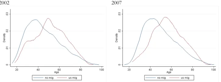
household with migrants had on average significantly less children than those without migrants. We also find that household heads of families that have migrants are older than the household heads of families without migrants. This tendency as displayed in Figure 2 reflects the general trend of children to migrate. The age distribution of heads from migrant households shifted to the left, indicating that households with very young household heads have a lower likelihood to have migrants compared to older households. It is also interesting that this trend is stable during the period the survey covered.

As can be seen in Table 2, only 31% (17%) of all households with international migrants in 2002 (2007) have a migrant household head. Migrants are mostly male household members with an average age of 32.6 (33.2) years. The high average migration duration reflects the fact that two thirds of the households in 2007 had at least one member who spent the last 12 months entirely abroad. Unfortunately we have no measure that captures their return intentions. The most important aspect in Table 2 is that it is mostly sons and daughters who migrate. When we split these statistics by the average age of the household head of migrant households (i.e. 56 years) it becomes even more explicit that in older households mostly the household heads' children migrated.

The survey asked households whether remittances were sent for a specific purpose, i.e. earmarked for a certain use. Interestingly only around 4% of the remittance receiving households stated that remittances were sent for the purchase of production inputs, livestock or land. All other households stated that remittances were sent to cover debt repayment, daily expenditures as well as health and schooling expenditures. It is also important to note that only around 12% of the households had a debit, credit or savings account in 2007. To cover large lump sum investments the households would then have to hold all savings in cash which might be too risky. The stated preference for daily expenditures could therefore also reflect the inaccessibility of an adequate savings vehicle.

Following the literature we separate investment alternatives into two logically coherent categories: agriculture and livestock. The former includes investments in agricultural assets such as expenditures to improve the plot and the installation of irrigation systems, acquisition of new machinery as well as expenditures to maintain productive assets. Investments in livestock include expenditure categories such as the acquisitions of new livestock and expenditures for new

(12)

machinery. About one-third of the households invested productively5_{. The households with}

international migrants seem to have slightly higher propensities to invest in agricultural assets and livestock. Regarding the investment shares, neither category stands out. While livestock makes up the biggest part of investments in terms of frequency, agriculture seems to account for the bigger share in total investment volumes in both years. Unfortunately the survey data does not allow us to analyze the stocks and investment flows of other income generating activities.

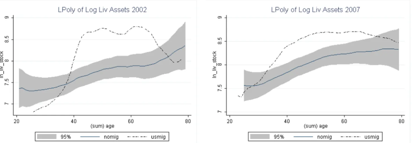
Given that the age of household heads differs markedly between non-migrant and migrant households, as observed in Table 1, the subsequent question is whether this pattern holds for the households’ investment activities. In Figures 3 we capture the relationship between investment status and the age of the household head differentiated into households that had no migrants and those that had international migration. The graphs reveal two things. First, households with international migrants seem to hold more agriculture and livestock assets in both years. Second, especially for livestock assets we observe a strong curvature that indicates a life-cycle investment structure. More precisely, the value of livestock increases up to the age of around 40 years of the household head and remains quite stable until the age of 60. Thereafter households seem to hold less livestock.

IV. Econometric Strategy

Econometrically the relation between investments and migration has been previously approached using a simple setup. Typically a certain type of investment is regressed on remittances controlling for household characteristics to account for their heterogeneity. However, this ignores the variables highlighted by the financial theory of investment, i.e. the importance of internal sources of finance in imperfect capital market situations (Hubbard 1998). By rearranging equation (4) it becomes clear that investments are determined by

⋅ , (10)

The investment equation we test differs from previous agricultural investment estimations (e.g. Elhorst 1993, Hubbard and Kashyap 1992) in two aspects. First, due to data limitations we cannot include some commonly used indicators. More precisely, we cannot include any measure of output or factor input prices. Yet this should not affect our estimates because although factor

(13)

prices are most likely heterogeneous across regions it is unlikely that households in the same states face significantly different factor prices. The variation between communities should be absorbed to a large extent by state fixed effects. We also include only agricultural and livestock sales as a proxy for cash flows since we do not observe directly the savings or changes in inventories of households. We also deviate from the common approach where investments are estimated as a share of total capital. The reason for this deviation lies in the structure of our data. As outlined before the survey did ask explicit questions about investments. However the categories used in these investment questions do not perfectly match the categories about productive household assets. Second, we do not have any measure of market opportunities in the form of fundamental q as it is commonly used in investment analysis (e.g. Bierlen and Featherstone 1998). However, this should not be a problem since we approach the data with a reduced form and do not derive a structural interpretation from the estimation model. In addition, the structural derivation of the q-model assumes perfect competition and constant returns to scale which would be unrealistic in our context. Taking these limitations into account our general estimation equation takes the following form:

log i=1,…,N; t=1,2; (11)

Where I is investment or an investment good, X is a vector of household characteristics, K is capital and C represents cash flows. The variable of interest is migration (M). Household characteristics consist of the number of adults in the household as well as the age and education of the household head. We also included a squared age term for the household head to capture potential non-linear effects. Throughout all estimations the quadratic term should not have any statistical significance if there are no life-cycle effects. The capital vector contains the capital stocks of the household, i.e. the aggregated value of agricultural assets and the value of the livestock the household owned. These stocks are not only important as a measure of productive capacity but also because they reflect the wealth of the household. This duality makes this measure somewhat ambiguous as it indicates both, the production setup and degree of specialization, as well as the accumulated wealth of the household. The vector C describes the households' cash flows and access to capital. Again the interpretation of the elasticity of investment with respect to cash flows is difficult since these variables contain different types of information. On the one hand they reflect the internal financing capacity of the household represented by cash flows vis-á-vis the external capital in form of credits. On the other hand cash flows could also represent future investment opportunities and market conditions instead of the

(14)

role of internal funds (Gilchrist and Himmelberg 1995). But since the objective of this analysis is not to determine whether households are credit constrained due to imperfect capital markets, the size of the effect is not of primary importance. Rather, the difference in the importance of cash flows for migrants and non-migrants is sufficient to test if migration provides capital for investment and thereby changes the financing structure of investments. It is worth noting that while this investigation focuses on capital expenditures it is also possible that cash flows are used to finance other production relevant categories such as cash holdings, increases in inventories or of non-farm activities.

Additionally to the theoretical reasons why farmers do not invest as outlined in section two of this paper there are also some empirical reasons why we might not observe investments. Most likely, capital investments are quite infrequent which is why the observation period of a single year cannot fully reflect the investment activity of a farmer. It is also possible that unobservable factors are driving the investment decision. For example, transaction cost can be too high due to the remote location of some municipalities or the overall market situation depresses the expectations of the farmer. Unfortunately we have no way to clearly identify the cause of zero observations in our investment flows. However the exclusion of households with zero investments for a given year would imply zero demand which is not necessarily true. If the selection into the observable subgroup is nonrandom OLS estimates are inconsistent. We use two techniques to address this problem. First, we use not only investment flows but also capital stocks which are by definition the result of all prior investment flows. Second, we use a Tobit model which produces consistent parameter estimates in the presence of a truncated dependent variable (Amemiya 1973).

We begin the analysis by pooling the data set to evaluate the changes of investment between the years i.e. the effect of time. This also allows us to check for attrition. By including a dummy that indicates if the household was observed in 2007, we can evaluate systematic differences of attriters. As pointed out by Arslan and Taylor (2011) attrition can be caused by (non-random) whole-household migration. If this was indeed the case the estimations of our migration coefficients would be upward biased since these migrant households did not invest in agricultural assets but are unobservable in the second survey round.

To exploit the advantage of having two periods we then employ a Lagged Dependent Variable (LDV) estimation. This approach helps us to control for events that happened prior to the period

(15)

of observation and possibly influenced investment behavior permanently, but also to capture slow changing or invariant characteristics of the household such as entrepreneurial abilities and risk attitudes. Hence, the LDV must be understood as a proxy for all unobserved time-invariant variables that affect investment. One problem of this approach is the possible correlation of the lagged dependent variable with the error term. The bias introduced by this correlation shifts the coefficients of our explanatory variables toward zero (e.g. Griliches 1961). However, since we are neither relying on the point estimate of the lagged investment variables nor emphasizing the coefficient size of the other variables too much, there is no reason to refrain from using lagged variables. We should understand the LDV parameter estimates as the lower bound of the possible effects.

The main advantage of the panel structure of our dataset is that it allows us to control for constant and slow changing household specific effects. Both, our pooled OLS and our LDV estimates would be biased and inconsistent in the presence of unobserved individual heterogeneity. To address this problem we also employ fixed effects estimation. However, since we are restricted to two periods this estimation is equivalent to first differences and only captures the effect of variation within our unit of observation. In our sample 203 households decided to migrate after 2002 and 76 households ceased to have migrants in 2005. The FE estimation thus represents a comparison of new migrants and households that have concluded their migration activities. 6

The central problem for the identification of the effect of migration in all of these setups is the non-random selection of households into migration. More precisely households that have migrants might be systematically different from those that do not. This intuition is supported by a simple Durbin-Wu-Hausman Chi² test which rejected the exogeneity of our migration indictor in almost all regressions. For Mexico various migration instruments have been used successfully, among them migration networks (Chiodi et al. 2012), historic state-level migration rates (Woodruff and Zenteno 2007, Taylor and Lopez-Feldman 2010), and migrant-weighted economic conditions at the destination (Orrenius et al. 2010, Arslan and Taylor 2011). We employ the number of years since the first migration occurred in each community. This variable reflects the age of the network and therefore the level of migration costs. Following the argumentation by McKenzie and Rapoport (2007) we expect migration probability to increase

6_{We do not report our random effects estimation since after controlling for year and state fixed effects the results}

(16)

with the age of the network.7_{In addition to using the age of existing migration networks, which}

partly captures the effect of historic migration, we construct an instrumental variable based on the U.S. state-level GDP growth weighted by the number of migrants each community had in 2002 and 2007 in different states.

⋅∑ ⋅ j=1,…,60 (12)

Hence, the instrumental variable for household i, in village j, is a weighted average of the GDP growth in all states D the community had a migration network with at time t. The assumption behind this instrument is that increased economic activity is strongly correlated with higher wages and a higher probability of finding employment for a migrant. There is no reason to believe that economic growth in U.S. states affects the investment activity in specific Mexican communities. This exclusion restriction would only be violated if for example farmers would market their production in the United States as well which is unlikely since the households in our sample are small scale producers and only cater to local markets.

Since we are not able to address the endogeneity of migration in the Tobit model due to the binary nature of our migration variable we follow the recommendation by Angrist (2001) to employ a conventional two-stage least squares (2SLS) estimation. In addition to obtaining consistent parameter estimates, this also allows us to perform a broad range of tests regarding the strength and validity of our instrumental variables. The Hansen J test cannot reject the hypothesis that our instruments are uncorrelated with the error term. We can therefore accept the orthogonality conditions required for our instruments to be valid but this does not tell us how strong their predictive power is. To evaluate the strength of our instrument we use the Kleinbergen-Paap test of under-identification and the Cragg-Donald F-statistic of our first stage. We report both tests in the last two rows of each table and find that our instruments are jointly significant throughout. Furthermore the Cragg-Donald F-statistic mostly exceeds the critical 10% value for weak instruments proposed by Stock and Yogo (2001) that stands at 19.93 for our specifications. Overall, these tests confirm the adequacy of our two instruments.

Our estimation and instrumentation strategy has two important implications that should be considered before we turn to the results. First, a system estimation approach could help us to

7_{The variable also captures the effect of the exogenous Bracero program indirectly. The communities with the oldest}

(17)

gain efficiency in our estimations. However, we found only a very small correlation of agriculture and livestock residuals. This observation and our primary interest in migration shift the balance in favor of a single-equation approach in this context. Albeit being less efficient our single-equation estimations remain consistent when estimated independently. Second, the 2SLS estimation model can only yield local average treatment effect (LATE) estimates since some households are defiers in that they do not react to changes in the market conditions at the destinations. One way to overcome this limitation and also investigate the possible heterogeneity of other explanatory variables in both migrant and non-migrant households is to employ an endogenous switching regression model (SRM) which is a generalization of a Heckman selection correction (Heckman 1979). In doing so we are using a control function in form of the inverse Mill’s ratio that is added to equation (11). The exogenous variables used to derive the inverse Mill’s ratio are the same we use in the 2SLS specification (see equation 12). This approach also allows us to observe the effect of age separately for migrant and non-migrant households without using instrumented interaction terms which could possibly suffer from decreased efficiency due to the lower correlation between the interacted endogenous migration variable and the interacted instrument.

V. Estimation Results

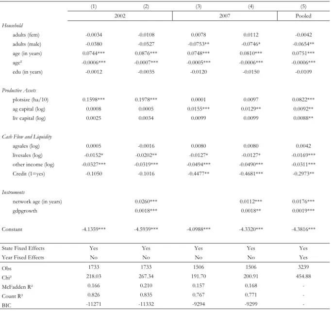
To evaluate the migration decision process that underlies our instrumental variable strategy we display our Probit estimates of having an international migrant in the household in Table 3. After augmenting the basic setup with our migration instruments the estimated coefficients show that the exogenous instruments have significant effects on the propensity to migrate. We find that the age of the migration network increases the propensity to migrate. Similarly, the growth of GDP at the destination states weighted by the size of the diasporas increases the likelihood of having at least one migrant in the household. For both years we find that the probability of migration first increases with age and decreases after a turning point of around 61 and 72, in 2002 and 2007, respectively, keeping all other variables constant. When examining economic characteristics of the households, we find strong evidence that international migration is associated strongly with current income flows. Higher current income from livestock sales and non-farm activities significantly reduces the probability that the household has at least one international migrant. Agricultural sales have no statistically significant relation with the propensity to migrate. By contrast, we find that agricultural assets have a slightly positive correlation with the probability of having an international migrant in the household. This could reflect asymmetric migration costs which would imply that only wealthier households are able to cover these costs. A second

(18)

interpretation that does not conflict with the first is that mostly the wealthier households start investing in more profitable activities such as migration.

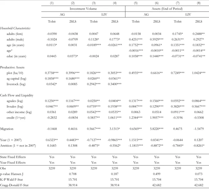
In Table 4 we report the estimation results for the pooled estimations of both, the investment flows and stocks. The agricultural investment intensity seems to be independent of age while livestock investment flows decrease significantly with age. This could indicate that most households rely on agriculture for their daily consumption throughout the life-cycle. The asset accumulation follows a clear life-cycle pattern for both agricultural and livestock assets, peaking at the age of 48 and 63 in the 2SLS specification, respectively. Apart from the age of the household head all production characteristics, i.e. productive assets and cash flows, are practically and statistically important determinants of investment behavior. The cash flow elasticity of investment of both agriculture and livestock is throughout strongly category specific. That is, investments in livestock are more sensitive to profits from livestock sales than from retained agricultural profits. Plot size as well as the value of agricultural assets and livestock have robustly positive effects. This result does not reject the decreasing returns to capital as predicted by theory but rather reflects the fact that our investment variable contains replacement expenditures. Furthermore if we use the share of investment as independent variable the asset coefficients have a negative sign. The year fixed effects show that both agricultural investments and assets are higher in the second wave in 2007. From the attrition indicator we see that households that were not surveyed in 2007 seem to be characterized by slightly lower investments and assets throughout. In both the Tobit and the 2SLS specification, international migration seems to have a slightly positive effect on livestock investment flows and a robustly positive effect on agricultural assets.

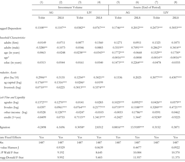
Table 5 reports the results for the Lagged Dependent Variable estimation. The lagged variable is also an indicator of the persistence of investment activities. That is, it measures how strongly current investment depends on past investments. The strong difference between flows and stock can be interpreted as an indication of an infrequent and lumpy adjustment process of capital. Specifically for livestock, we can observe that past investments have a low predictive power of current investments, whereas our asset measure is quite persistent. Almost all of the results observed in the pooled specification regarding the demographic structure of investments, the importance of cash flows and the effect of migration remain unchanged.

(19)

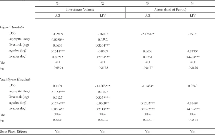
The results of Tables 4 and 5 suggest that the internally generated cash flows by market integration of the rural households in the form of sales are more important for the accumulation of livestock than the funds generated by the migration of household members, while agricultural asset accumulation clearly benefits from migration. However, to find out if the age of the household head and the cash flows the household receives have different effects in migrant and non-migrant households the estimates provided by our 2SLS specifications do not suffice. If migration in fact injects capital for investment only for specific types of agricultural production we should observe marked differences in cash flow sensitivity between migrant and non-migrant households. To test this hypothesis we turn in Table 6 to the split sample parameter estimates obtained through the switching regression model. We find that the correlation coefficient of the error terms in the selection and regression equation (rho) is throughout negative for migrant households. This confirms that the households with migrants are positively selected in terms of the two instruments and are more likely to have higher investments and more accumulated assets than a household drawn at random from the population mirroring the results obtained from the 2SLS specification as reported in Table 4.

Table 6 yields two important insights. First, the estimated elasticity of agricultural investment to changes in category specific cash flows represented by sales for households without migrants is 12,4%. Migrant households show an elasticity of about 15.1%. The difference is very small and statistically insignificant. The same is true for livestock investments and assets. In the NELM literature it is generally argued that remittances are used to overcome these financing constraints. The comparison of the cash flow coefficients across the two subsamples of migrant and non-migrant households in Table 6 shows that the cash flow sensitivity does not vary systematically across households. Only for agricultural assets we see that the cash flow sensitivity becomes statistically insignificant for migrant households. While this evidence does not allow us to judge the extent of the existing credit constraints, it allows us to reject the hypothesis that funds generated by migration change the capital demand of farm households indiscriminately, but only for agricultural activities. Second, to find out if migrant households’ investment behavior follows a pattern that is consistent with the permanent income hypothesis more strongly than non-migrant households as indicated by the profile plots in Figure 3 we included an old age dummy, reflecting the mean age of household heads in 2007, instead of the continuous age variable in the switch regression model. We see that although the coefficient of the age dummy is negative for all specifications of migrant households, it is only significant for agricultural assets. A comparison of migrant and non-migrant households indicates that migrant households seem to disinvest

(20)

more strongly during old age than non-migrant households. However, since this finding is not very robust we have to regard it with caution.

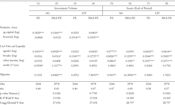
Table 7 shows the results from the fixed effects estimation of agricultural and livestock investments and capital stocks. Since the demographic characteristics of the household, i.e. age, composition and education, as well as plot size can be considered fixed over the short period of our observation we did not include them. We find that agricultural and livestock sales are again positive and significant at the 1% level for the respective asset category throughout. International migration has again a positive and highly significant effect on agricultural assets in both the standard and the instrumented fixed effect specification. We also observe a strongly positive effect of migration on agricultural investments and a negative effect on livestock investments in the 2SLS specification. Since these parameter estimates are based on the comparison between households that had a migrant in 2002 but none in 2007 and households that started to migrate in 2007 we can conclude that revenues from migration are indeed only used to build up the subsistence category of agricultural production. The negative coefficient of livestock investments can be interpreted as suggestive evidence that migration serves as a substitute for livestock production.

To summarize, we find that migration has strong positive effects on agricultural assets but not so much on livestock. Agricultural assets are built up with the capital received from migration. These effects are statistically significant, robust to changes in the specification of our estimation equation and are also practically significant since they have stronger effects than most of the other variables included. The estimates based on investment flow variables do not show a clear pattern, possibly due to their more volatile and infrequent nature. Our estimations also show that livestock seems to be driven more consistently by life-cycle effects than agriculture where we cannot observe a robust effect of age on investments and capital stocks. One possible interpretation of these findings is that livestock and migration are substitutes while agriculture seems to be a subsistence category that will never be excluded from the income portfolio since it guarantees a minimum level of consumption. This would explain why we do not observe strong life-cycle effects for agriculture but a strongly positive effect of migration on agricultural asset accumulation. In the context of our theoretical framework, these results support the argument that households adjust their income portfolio and use migration as a profitable investment alternative. A different reading of our results, which does not invalidate the subsistence hypothesis, is that livestock also serves as a risk buffer as argued by Dercon (1998) for the case of

(21)

rural Tanzania. This essential insurance function of livestock could become obsolete and no investments would take place if migration had a risk diversifying effect.

VI. Conclusion

This paper addresses the predictions of NELM theory that remittances increase productive investments if credit constraints are binding for the migrant sending households. We explored three aspects that have so far not received enough attention in the literature regarding the nexus of migration and investments and that could possibly reconcile the contradicting results in the empirical literature on remittances and investments: the distinction between different productive investment categories, cash flows as fundamental investment determinants and possible life-cycle effects as important investment constraints. We employ various econometric techniques to investigate the effect of international migration on investment volumes and accumulated capital stocks.

After ruling out that our results are driven by selection or endogeneity, we take away three important findings from our investigation. First, life-cycle effects may inhibit an increase in investments. Our estimates show strong live-cycle effects but no systematic difference between migrant and non-migrant households. We found some evidence that migrant household disinvest more strongly at the later stage of their life-cycle than non-migrant households. This observation calls for an explicit consideration of the stage of the migration cycle in future research regarding the effect of international migration on productive investments and asset accumulation. If migration occurs at a late stage of the life-cycle there is no reason to expect strong investments since the horizon for the returns to investments become shorter. Second, production fundamentals appear to be very important. Throughout category specific cash flows are the most predictive indicator of investments. Since all of the cash flows we observe are generated through market sales we have to conclude that market integration remains the strongest driver of investment. Third, pooling different investment categories distorts the causal relationship underlying the estimation. While our results indicate that migrants have accumulated more agricultural productive capital this is not the case for livestock, indicating that most households rely on agriculture for their daily consumption throughout the life-cycle. We should not expect strong investments in agriculture in general but only in the activities that secure the subsistence of the household.

(22)

Literature

Adams, R. (1998). Remittances, investment, and rural asset accumulation in Pakistan. Economic

Development and Cultural Change, 47(1), 155-173.

Ahituv, A. and Kimhi, A. (2002). Off-farm work and capital accumulation decisions of farmers over the life-cycle: the role of heterogeneity and state dependence. Journal of Development

Economics, 68(2), 329-353.

Amemiya, T. (1973). Regression analysis when the dependent variable is truncated normal.

Econometrica, 41(6), 997-1016.

Angrist, J. (2001). Estimation of limited-dependent variable models with binary endogenous regressors: simple strategies for empirical practice. Journal of Business and Economic Statistics, 19(1), 2-16.

Arslan, A. and Taylor, J.E. (2011). Whole household migration, inequality and poverty in rural Mexico. Kiel Working Paper No. 1742, Kiel Institute for the World Economy.

Bierlen, R. and Featherstone, A. M. (1998). Fundamental q, cash flow, and investment: Evidence from farm panel data. Review of Economics and Statistics, 80(3), 427-435.

Chiodi, V., Jaimovich, E. and Montes-Rojas, G. (2012). Migration, remittances and capital accumulation: Evidence from rural Mexico. Journal of Development Studies, 48(8), 1139-1155. Damon, A. (2010). Agricultural land use and asset accumulation in migrant households: the case

of El Salvador. Journal of Development Studies, 46(1), 162-189.

Davies, S., Easaw, J. and Ghoshray, A. (2009). Mental accounting and remittances: A study of rural Malawian households. Journal of Economic Psychology, 30(3), 321-334.

De Brauw, A. and S. Rozelle (2008). Migration and household investment in rural China. China

Economic Review, 19(2), 320–335.

Démurger, S. and Xu, H. (2011). Return migrants: The rise of new entrepreneurs in rural China.

World Development, 39(10), 1847-1861.

Dercon, S. (1998). Wealth, risk and activity choice: cattle in western Tanzania. Journal of

Development Economics, 55(1), 1-42.

Dustmann, C. (1997). Return migration, uncertainty and precautionary savings. Journal of

Development Economics, 52(2), 295-316.

Dustmann, C. and Kirchkamp, O. (2002). The optimal migration duration and activity choice after remigration. Journal of Development Economics, 67(2), 351-72.

Elhorst, P.J. (1993). The estimation of investment equations at the farm level. European Review of

Agricultural Economics, 20(2), 167-182.

Fazzari, S., Hubbard, G. and Petersen, B. (1988). Financing constraints and corporate investment. Brookings Papers on Economic Activity, 1, 141-206.

(23)

Gollier, C. and Zeckhauser, R. (2002). Horizon length and portfolio risk. Journal of Risk and

Uncertainty, 24(3), 195-212.

Griliches, Z. (1961). A note on serial correlation bias in estimates of distributed lags. Econometrica, 29(1), 65-73.

Heckman, J. (1979). Sample selection bias as a specification error. Econometrica, 47(1), 153-161. Hubbard, R. G. and Kashyap, A.K. (1992). Internal net worth and the investment process: an

application to U.S. agriculture. Journal of Political Economy, 100(3), 506-534.

Hubbard, R.G. (1998). Capital-market imperfections and investment. Journal of Economic Literature, 36(1), 193-225.

Ilahi, N. (1999). Return migration and occupational change. Review of Development Economics, 3(2), 170–186.

Lamb, R. (2003). Fertilizer use, risk, and off-farm labor markets in the semi-arid tropics of India.

American Journal of Agricultural Economics, 85(2), 359–371.

Lucas, R. and Stark, O. (1985). Motivations to remit: Evidence from Botswana. Journal of Political

Economy, 93(5), 901–918.

McCormick, B. and Wahba, J. (2003). Return international migration and geographical inequality: The case of Egypt. Journal of African Economics, 12(4), 500-532.

Mckenzie, D. and Rapoport, H. (2007). Network effects and the dynamics of migration and inequality: Theory and evidence from Mexico. Journal of Development Economics, 84(1), 1-24. McKenzie, D. and Rapoport, H. (2010). Self-Selection patterns in Mexico-U.S. migration: The

role of migration networks. Review of Economics and Statistics. 92(4), 811-821.

Mendola, M. (2008). Migration and technological change in rural households: Complements or substitutes? Journal of Development Economics, 85(1-2), 150-175.

Mesnard, A. (2004). Temporary migration and capital market imperfections. Oxford Economic

Papers, 56(2), 242-262.

Orrenius, P., Zavodny, M., Cañas, J. and Coronado, R. (2010). Do remittances boost economic development? Evidence from Mexican states. Law and Business Review of the Americas, 16(4), 803-821.

Piracha, M. and Vadean, F. (2010). Return migration and occupational choice: Evidence from Albania. World Development, 38(8), 1141-1155.

Quisumbing, A. and McNiven, S. (2010). Moving forward, looking back: The impact of migration and remittances on assets, consumption, and credit constraints in the rural Philippines. Journal

of Development Studies, 46(1), 91-113.

(24)

Stock, J. H. and Yogo, M. (2001). Testing for Weak Instruments in Linear IV Regression. NBER Technical Working Paper No. 284.

Taylor, J. E. (1999). The new economics of labor migration and the role of remittances in the migration process. International Migration, 37(1), 63-88.

Taylor, J. E., Rozelle, S. and De Brauw, A. (2003). Migration and incomes in source communities: A new economics of migration perspective from China. Economic Development and Cultural

Change, 52(1), 75-101.

Taylor, J. E. and Lopez-Feldman, A. (2010). Does migration make rural households more productive? Evidence from Mexico. Journal of Development Studies, 46(1), 68-90.

Woodruff, C. and Zenteno, R. (2007). Migration networks and microenterprises in Mexico.

Journal of Development Economics, 82(2), 509-528.

Wouterse, F. and Taylor, J. (2008). Migration and income diversification: Evidence from Burkina Faso. World Development, 36(4), 625-640.

Yang, D. (2008). International migration, remittances, and household investment: Evidence from Philippine migrants’ exchange rate shocks. Economic Journal, 118, 591-630.

Zeldes , S. (1989). Consumption and liquidity constraints: An empirical investigation. Journal of

(25)

Annex

Table 1: Household Characteristics

(1) (2) (3) (4) (5) (6) (7) (8)

2002 2007

all nonmig mig Pr(diff!=0) all nonmig mig Pr(diff!=0)

HH Size 4.48 4.53 4.28 0.07 4.25 4.35 3.98 0.01

Children (<16) 1.55 1.61 1.30 0.00 0.94 1.02 0.72 0.00

Sex of HH Head (1 = male) 0.86 0.86 0.86 0.78 0.84 0.84 0.83 0.51

Age of HH Head 48.93 47.81 53.54 0.00 53.44 51.49 58.54 0.00

Years of Education of HH Head 4.50 4.67 3.79 0.00 4.64 4.93 3.87 0.00

Income per Capita (in LCU) 11978.00 10359.77 18648.47 0.01 15525.96 12991.32 22157.79 0.01

of which (in %) Agriculture 0.09 0.09 0.09 0.76 0.08 0.08 0.08 0.95 Livestock 0.04 0.04 0.05 0.68 0.05 0.05 0.04 0.52 Non-Agricultural Business 0.07 0.08 0.07 0.36 0.07 0.08 0.06 0.16 Agricultural Wages 0.17 0.19 0.12 0.00 0.16 0.19 0.11 0.00 Non-Agricultural Wages 0.27 0.31 0.11 0.00 0.23 0.27 0.13 0.00 Transfers 0.14 0.14 0.11 0.01 0.17 0.18 0.13 0.00 International Remittances 0.07 0.00 0.38 0.00 0.10 0.00 0.36 0.00

Ag. Machinery (in LCU) 4722.18 3937.44 7956.93 0.00 8785.09 6633.54 14414.53 0.00

Livestock (in LCU) 8579.83 6778.10 16006.72 0.01 11186.22 9468.88 15679.57 0.00

Priv. Land (in ha) 1.10 1.01 1.50 0.43 1.44 1.43 1.46 0.97

International Migration (US) 0.20 0.00 1.00 - 0.28 0.00 1.00 -

Obs 1762 1418 344 - 1537 1112 425 -

Note: All income figures are in constant 2003 Mexican pesos and include negative incomes. In 2003, 1 Mexican peso was worth USD 0.62.

Transfer income includes PROCAMPO, PROGRESA, transfers by non-governmental organizations and friends. For 2007 transfers also includes PROARBOL and PROGAN. Authors calculation based on ENRUM.

(26)

Table 2: Migrant Characteristics (1) (2) (3) (4) (5) all 2002 2007 <56 [pooled] >56 [pooled] Male 0.82 0.85 0.80 0.87 0.78 Age 32.96 32.64 33.21 30.19 35.54 Primary Education 0.49 0.55 0.45 0.48 0.51 Secondary Education 0.30 0.26 0.33 0.32 0.28 Married 0.60 0.63 0.57 0.55 0.64

Average Annual Migration Duration 10.05 9.41 10.55 9.42 10.62

Years of Migration Experience 7.80 7.85 7.70 6.24 9.19

Migrants per Household 1.81 1.43 2.02 1.42 2.07

HH Head (male) 0.24 0.31 0.17 0.43 0.06

HH Head (female) 0.02 0.02 0.01 0.03 0.00

Daughter (at least 1) 0.25 0.18 0.29 0.15 0.33

Son (at least 1) 0.68 0.59 0.71 0.50 0.81

Other relative 0.05 0.03 0.07 0.04 0.06

Obs 737 326 411 370 367

(27)

Table 3: Migration Determinants (Probit) (1) (2) (3) (4) (5) 2002 2007 Pooled Household adults (fem) -0.0034 -0.0108 0.0078 0.0112 -0.0042 adults (male) -0.0380 -0.0527 -0.0753** -0.0746* -0.0654**

age (in years) 0.0744*** 0.0876*** 0.0748*** 0.0810*** 0.0751***

age² -0.0006*** -0.0007*** -0.0005*** -0.0006*** -0.0006***

edu (in years) -0.0012 -0.0035 -0.0120 -0.0150 -0.0109

Productive Assets

plotsize (ha/10) 0.1598*** 0.1978*** 0.0001 0.0097 0.0822***

ag capital (log) 0.0008 0.0005 0.0155*** 0.0129** 0.0092**

liv capital (log) 0.0025 0.0034 0.0099 0.0099 0.0088**

Cash Flow and Liquidity

agsales (log) 0.0005 -0.0016 0.0080 0.0080 0.0042

livesales (log) -0.0152* -0.0202** -0.0127* -0.0127* -0.0169***

other income (log) -0.0327*** -0.0319*** -0.0494*** -0.0490*** -0.0311***

Credit (1=yes) -0.1050 -0.1016 -0.4477** -0.4681*** -0.2973**

Instruments

network age (in years) 0.0260*** 0.0112*** 0.0176***

gdpgrowth 0.0018*** 0.0018** 0.0019***

Constant -4.1359*** -4.5939*** -4.0988*** -4.3320*** -4.3816***

State Fixed Effects Yes Yes Yes Yes Yes

Year Fixed Effects No No No No Yes

Obs 1733 1733 1506 1506 3239 Chi² 218.03 267.34 191.70 200.91 454.88 McFadden R² 0.166 0.210 0.157 0.168 - Count R² 0.826 0.835 0.767 0.771 - BIC -11271 -11332 -9294 -9299 -

Note: Dependent variable is one if household has a member living or working more than three month per year in the US and zero otherwise; *

significant at 10%, ** significant at 5%, *** significant at 1%; T-statistics (two-tailed) based on robust standard errors. Authors calculation based on ENRUM.

(28)

Table 4: Pooled

(1) (2) (3) (4) (5) (6) (7) (8)

Investment Volume Assets (End of Period)

AG LIV AG LIV

Tobit 2SLS Tobit 2SLS Tobit 2SLS Tobit 2SLS

Household Characteristics

adults (fem) -0.0390 -0.0438 0.0047 0.0648 -0.0158 0.0034 0.1745* 0.2488**

adults (male) -0.1024 -0.0709 0.1128* 0.1773* 0.4251*** 0.5929*** 0.2631** 0.2927*

age (in years) 0.0113* 0.0031 -0.0189*** -0.0261*** 0.1752*** 0.0961* 0.1351*** 0.1832**

age² -0.0016*** -0.0010** -0.0011** -0.0014**

educ (in years) 0.0443 0.0373* -0.0024 0.0287 0.1058*** 0.1440*** -0.0731** -0.0741**

Productive Assets

plot (ha/10) 0.3758*** 0.3996*** 0.1826*** 0.3053*** 0.4935*** 0.6616** 0.7249*** 1.0424***

ag capital (log) 0.1858*** 0.1680*** 0.0260** 0.0361**

livestock (log) 0.0342* 0.0085 0.2942*** 0.3400***

Cash Flow and Liquidity

agsales (log) 0.1250*** 0.1167*** 0.0250** 0.0404** 0.1317*** 0.1560*** 0.0592*** 0.0864***

livsales (log) 0.0467** 0.0609** 0.0759*** 0.1938*** 0.0847*** 0.1290*** 0.3820*** 0.5667***

other income (log) 0.0361 0.0289 0.0542*** 0.0535** 0.0063 0.0514 0.0911*** 0.0662

credit (1=yes) -0.2832 -0.0834 0.5837** 1.0611*** 1.2344*** 1.9057*** -0.3196 -0.5308

Migration -0.1468 0.4616 0.5667*** 3.1313* 0.6569** 5.8220*** 0.4675 -1.5479

Year (1 = 2007) 0.6323** 0.4483** -0.7127*** -0.9865*** 1.1515*** 0.8341** -0.0644 0.1207

Attrition (1 = not in 2007) 0.1683 0.1308 -0.4875* -0.5562* -1.1815*** -0.8872** -0.7845* -0.8261*

State Fixed Effects Yes Yes Yes Yes Yes Yes Yes Yes

Year Fixed Effects Yes Yes Yes Yes Yes Yes Yes Yes

Obs 3239 3239 3239 3239 3239 3239 3239 3239

p-value Hansen J 0.708 0.187 0.499 0.073

K-P Wald F-Stat 15.701 15.701 15.704 15.704

Cragg-Donald F-Stat 38.914 38.914 42.682 42.682

Note: Dependent variables in logs; * significant at 10%, ** significant at 5%, *** significant at 1%; Tobit estimates are marginal effects (conditional on

being uncensored); all censored observations are left-censored at zero; T-statistics (two-tailed) based on robust standard errors clustered at the village level. Authors calculation based on ENRUM.

(29)

Table 5: Lagged Dependent Variable

(1) (2) (3) (4) (5) (6) (7) (8)

AG LIV AG LIV

Tobit 2SLS Tobit 2SLS Tobit 2SLS Tobit 2SLS

Lagged Dependent 0.1108*** 0.1107** 0.0382** 0.0767*** 0.1746*** 0.2012*** 0.2473*** 0.3053***

Household Characteristics

adults (fem) -0.0149 -0.0711 0.0877 0.1560 0.1271 0.0911 0.1325 0.1875

adults (male) -0.3280** -0.1073 0.0546 0.0883 0.3519** 0.7091*** 0.2862** 0.3414**

age (in years) 0.0063 -0.0248 -0.0238*** -0.0343** 0.1772*** -0.0668 0.1529** 0.1750*

age² -0.0016*** -0.0000 -0.0014** -0.0016**

educ (in years) 0.0313 0.0544 0.0161 0.0540 0.1473*** 0.2264*** -0.0478 -0.0355

Productive Assets

plot (ha/10) 0.2906** 0.3135 0.1254** 0.3021** 0.1536 0.2025 0.3077*** 0.4307***

ag capital (log) 0.1760*** 0.1316*** 0.0206* 0.0199

livestock (log) 0.0710*** 0.0225 0.3013*** 0.3374***

agsales (log) 0.1372*** 0.1270*** 0.0141 0.0283 0.1025*** 0.0992** 0.0426** 0.0579**

livsales (log) 0.0397 0.0961*** 0.0764*** 0.2177*** 0.0719*** 0.1188*** 0.3200*** 0.4721***

other income (log) 0.0528 0.1287** -0.0247 -0.0103 -0.0053 0.1786** 0.0591 0.0462

credit (1=yes) -0.8499 0.0755 0.7115** 1.3413*** -0.2427 1.3447 -0.9230* -0.9223

Migration -0.2498 6.1696 0.3058* 2.8312 0.8816*** 13.9189*** 0.3152 0.3871

State Fixed Effects Yes Yes Yes Yes Yes Yes Yes Yes

Obs 1487 1487 1487 1487 1487 1487 1487 1487

p-value Hansen J 0.9329 0.0639 0.4477 0.0922

K-P Wald F-Stat 9.192 8.645 10.084 10.370

Cragg-Donald F-Stat 9.992 9.403 11.957 11.375

Note: Dependent variables in logs; * significant at 10%, ** significant at 5%, *** significant at 1%; Tobit estimates are marginal effects (conditional on

being uncensored); all censored observations are left-censored at zero; T-statistics (two-tailed) based on robust standard errors clustered at the village level. Authors calculation based on ENRUM.

(30)

Table 6: Lagged Dependent Variable – Split Sample

(1) (2) (3) (4)

AG LIV AG LIV Migrant Households D58 _-1.2809 _-0.6002 _-2.4754** _-0.5331 ag capital (log) _0.0980** _0.0252 livestock (log) 0.0657 0.3554*** agsales (log) 0.1518*** -0.0109 0.0639 0.0790* livsales (log) _0.1021* _0.2233*** _0.0351 _0.4488*** Obs 411 411 411 411 rho -0.5594 -0.2178 -0.8177 -0.2626 Non-Migrant Households D58 _0.1191 _-1.1205*** _-1.1454* _0.0240 ag capital (log) 0.1752*** 0.0160 livestock (log) 0.0127 0.3339*** agsales (log) 0.1246*** 0.0509** 0.1202*** 0.0549* livsales (log) 0.0654** 0.2118*** 0.1392*** 0.4785*** Obs 1076 1076 1076 1076 rho 0.3223 0.3632 0.6650 -0.3874

State Fixed Effects Yes Yes Yes Yes

Note: Dependent variables in logs; Included control variables are number of adult women and men, education of the household head, plot size (ha/10),

(31)

Table 7: Fixed Effects

(1) (2) (3) (4) (5) (6) (7) (8)

AG LIV AG LIV

FE 2SLS-FE FE 2SLS-FE FE 2SLS-FE FE 2SLS-FE

Productive Assets

ag capital (log) _0.1820*** _0.1666*** _0.0255 _0.0465*

livestock (log) -0.0068 -0.0125 0.3314*** 0.3393***

agsales (log) _0.1053*** _0.0920*** _0.0323 _0.0505* _0.0777** _0.0391 _0.0652** _0.0614**

livsales (log) _0.0316 _0.0516* _0.1545*** _0.1272*** _0.0826*** _0.1259*** _0.3544*** _0.3585***

other income (log) _0.0333 _0.0408 _0.0242 _0.0139 _0.0863* _0.1007* _0.1057*** _0.1071***

credit (1=yes) _-0.9590* _-1.1677** _0.2091 _0.4951 _1.0863 _0.4961 _0.2360 _0.1792 Migration 0.1355 6.0482*** 0.2953 -7.8053** 0.9657* 16.3096*** 0.3083 1.7833 Obs 3244 2978 3244 2978 3244 2978 3244 2978 rho 0.40 0.45 0.40 0.47 0.47 0.49 0.58 0.57 p-value Hansen J 0.1426 0.7785 0.3620 0.1426 K-P Wald F-Stat 13.924 13.924 14.369 14.369 Cragg-Donald F-Stat 27.034 27.034 28.797 28.797

Note: Dependent variables in logs; * significant at 10%, ** significant at 5%, *** significant at 1%; T-statistics (two-tailed) based on robust standard

(32)

Figure 1: Interview Distribution

Figure 2: Age Distribution of Household Heads and Spouses by Migration Status

2002 2007

(33)

(34)

21