Survavibility in Multilayer Networks : models and Polyhedra

(1)

Universit´

e Paris-Dauphine

´

ECOLE DOCTORALE DE DAUPHINE

TH`

ESE

pr´esent´ee par

Raouia TAKTAK

pour obtenir le grade de

Docteur de l’universit´

e Paris-Dauphine

Sp´ecialit´e : Informatique

Survivability in Multilayer Networks:

Models and Polyhedra.

Soutenue publiquement le 04 juillet 2013 devant le jury :

A.R. Mahjoub Directeur de th`ese Universit´e Paris-Dauphine, France

V. Gabrel Co-encadrant Universit´e Paris-Dauphine, France

L. Gouveia Rapporteur Universidade de Lisboa, Portugal

A. Quilliot Rapporteur Universit´e Blaise Pascale, Clermont II, France

S. Borne Examinateur Universit´e Paris 13, France

E. Gourdin Examinateur Orange Labs, Issy-les-moulineaux, France

S.Th. McCormick Examinateur University of British Columbia, Canada

(2)

(3)

(4)

(5)

With the explosive growth of data traffic, telecommunication networks have evolved toward a model of high-speed IP routers interconnected by intelligent optical core net-works. Moreover, as telecommunication networks play a crucial role for the transfer of important data, they must present a minimum degree of survivability against acciden-tal breakdowns. One of the most useful strategies to ensure a network’s survivability, is to satisfy some connectivity requirements, that is to guarantee a certain number of disjoint paths between some pairs of the nodes in the network.

This thesis deals with a problem related to survivability issues in multilayer IP-over-WDM networks. Given a set of traffic demands for which we know a survivable logical routing in the IP layer, our purpose is to determine the corresponding survivable topology in the WDM layer. More precisely, suppose we are given an IP-over-WDM network with weights on the WDM layer, a set of demands and two-disjoint paths for each demand. The problem is to determine in the WDM layer a minimum weight subgraph containing two routing paths for each demand. These paths must be node-disjoint and go in the same order through the optical switches corresponding to the routers visited in the paths of the IP layer.

We show that in addition to its importance in the telecommunication context, the problem is very interesting from a theoretical point of view. We then prove that, under some conditions, the problem is NP-hard even for a single demand. Moreover, we propose four integer linear programming formulations for the problem. The first one, called cut formulation, is induced by the so-called cut inequalities which are in an exponential number. We carry out a polyhedral investigation of the convex hull of its feasible solutions. We identify several families of valid inequalities and discuss their facial aspect. We then devise separation routines for these inequalities and develop a Branch-and-Cut algorithm. The second formulation is a path formulation which uses the paths between the origin-destination of the demands’ sections. Based on this formulation, we devise a Branch-and-Price algorithm for the problem. In addition, we present a third formulation which only uses the design variables. This formulation is

(6)

given in the case when we only have 3 terminals. For 4 terminals and more, such a formulation seems to be a hard problem. Finally, the last formulation is a compact formulation which, in addition to the design variables, uses a further family of variables. We show that this formulation performs well and gives a tighter bound for the problem. Key words : IP-over-WDM networks, survivability, complexity, polytope, facet, Branch-and-Cut algorithm, Branch-and-Price algorithm, extended formulation.

(7)

Paralèllement à l’augmentation significative du volume des informations échangées, à la multiplication des services et à la diversification des données, les réseaux de télécommunications évoluent vers une structure multicouche qui s’avère la plus adaptée à tous ces changements. L’architecture IP-sur-WDM, exploitant la technologie de la fibre optique, présente en particulier une infrastructure prometteuse pour les réseaux futurs. De plus, étant impliqué dans le transport de données importantes, ces réseaux doivent être dotés d’un niveau de fiabilité suffisant, leur permettant de rétablir les connexions en cas de panne de l’un des équipements dans le réseau.

Dans cette thèse, nous nous intéressons à un problème de fiabilité dans les réseaux multicouches IP-sur-WDM. Etant donné un ensemble de demandes pour lesquelles on connaˆıt une topologie fiable dans la couche IP, le problème consiste à sécuriser la couche optique WDM en y cherchant une topologie fiable. Plus précisément, on suppose données un réseau IP-sur-WDM avec des poids sur la couche WDM, un ensemble de demandes et deux chemins sommet-disjoint routant chaque demande dans la couche IP. Le problème est de déterminer dans la couche WDM un sous-graphe de poids minimum contenant pour chaque demande deux chemins de routage. Ces chemins doivent être sommet-disjoints et doivent visiter les brasseurs de la couche WDM correspondant aux routeurs visités dans les chemins de la couche IP, tout en gardant le même ordre de passage.

Nous montrons que le problème est d’une importance cruciale non seulement d’un point de vue pratique mais aussi sur le plan théorique. Nous montrons que le problème est NP-complet même dans le cas d’une seule demande. Ensuite, nous proposons quatre formulations en termes de programmes linéaires en nombres entiers pour le problème. La première, dite formulation coupes, est induite par des inégalités dites de coupes et contient un nombre exponentiel de contraintes. Nous menons une investigation approfondie du polyèdre associé à cette formulation. Nous identifions de nouvelles familles de contraintes valides et étudions leur aspect facial. Nous décrivons également des procédures de séparation pour ces inégalités et développons un algorithme de coupes

(8)

et branchements pour le problème. Une deuxième formulation, basée sur les chemins et utilisant plutôt un nombre exponentiel de variables, est considérée dans un second temps. Nous proposons un algorithme de branchements et génération de colonnes pour cette formulation. Par la suite, nous discutons d’une troisième formulation qui utilise uniquement les variables naturelles du problème. Nous montrons que cette formulation est valide dans le cas de 3 terminaux par demande. Nous discutons aussi du cas de 4 terminaux et plus. Enfin, nous présentons une formulation étendue compacte qui, en plus des variables naturelles, utilise une autre famille de variables. Nous montrons que cette formulation fournit une bonne borne inférieure et permet de résoudre efficacement le problème.

Mots clés : Réseaux de télécommunications IP-sur-WDM, sécurisation, complexité, polytope, facette, algorithme de coupes et branchements, algorithme de branchements et génération de colonnes, formulation étendue.

(9)

Table of Contents x

Introduction 1

1 Preliminary notions 5

1.1 Combinatorial optimization . . . 6

1.2 Algorithmic and complexity theory . . . 7

1.3 Polyhedral approach and Branch-and-Cut . . . 8

1.3.1 Elements of the polyhedral theory . . . 8

1.3.2 Cutting plane method . . . 11

1.3.3 Branch-and-Cut algorithm . . . 13

1.4 Column generation and Branch-and-Price. . . 15

1.4.1 Column generation method . . . 15

1.4.2 Branch-and-Price algorithm . . . 16

1.4.3 Primal heuristics . . . 17

1.5 Extended Formulations . . . 18

1.6 Graph theory: definitions and notations . . . 20

2 Multilayer telecommunication networks 23 2.1 Telecommunication networks: toward a multilayer structure . . . 24

2.1.1 Evolution of networks’ architecture . . . 24

2.1.2 The IP layer . . . 26

2.1.3 The WDM layer. . . 31

2.1.4 Interactions between the IP and WDM layers . . . 34

2.2 Survivability concepts in multilayer networks . . . 36

2.2.1 Restoration . . . 36

(10)

2.2.3 Survivability in multilayer networks . . . 37

2.3 Multilayer network design and survivability. . . 38

2.3.1 The general survivable network design problem . . . 38

2.3.2 Multilayer survivable network design . . . 42

3 MSOND Problem: context and complexity 45 3.1 The MSOND problem . . . 46

3.1.1 Problem presentation . . . 46

3.1.2 Notations and examples . . . 47

3.1.3 Sections’ disjunction . . . 51

3.2 Theoretical context . . . 53

3.2.1 Shortest Path Problem with Specified Nodes . . . 53

3.2.2 Travelling Salesman Problem and its variants . . . 53

3.2.3 The k-Vertex Disjoint Paths Problem . . . 55

3.3 Complexity results . . . 56

3.3.1 Single commodity MSOND problem . . . 56

3.3.2 Multi-commodity MSOND problem . . . 61

3.3.3 Summary table . . . 63

3.4 Concluding remarks . . . 63

4 Cut formulation and polyhedra 65 4.1 Cut formulation . . . 66

4.2 Associated polytope . . . 68

4.2.1 Dimension . . . 68

4.2.2 Facial investigation . . . 74

4.3 Valid inequalities and facets . . . 96

4.3.1 Steiner cut inequalities . . . 97

4.3.2 Steiner non-successive terminals inequalities . . . 104

4.3.3 Steiner F-partition inequalities . . . 112

4.3.4 Generalized Steiner partition inequalities . . . 125

4.3.5 Generalized disjunction inequalities . . . 129

4.3.6 Steiner comb inequalities . . . 130

5 Branch-and-Cut algorithm 135 5.1 Branch-and-Cut algorithm . . . 136

(11)

5.1.1 Description . . . 136

5.1.2 Test of feasibility . . . 138

5.1.3 Separation of cut inequalities . . . 138

5.1.4 Separation of Steiner cut inequalities . . . 139

5.1.5 Separation of Steiner non-successive terminals inequalities . . . 139

5.1.6 Separation of Steiner F-partition inequalities . . . 144

5.1.7 Implementation’s features . . . 144 5.1.8 Branching strategy . . . 145 5.2 Computational study . . . 146 5.2.1 Computations’ context . . . 146 5.2.2 Description of instances . . . 146 5.2.3 Experimental results . . . 148 5.2.4 A French instance. . . 153 5.3 Concluding remarks. . . 154

6 Path formulation and Branch-and-Price algorithm 159 6.1 Path formulation . . . 160

6.1.1 Section formulation . . . 160

6.1.2 Dantzig-Wolf decomposition . . . 161

6.1.3 Path formulation . . . 162

6.2 Cut versus path formulation . . . 164

6.2.1 Relation between variables . . . 164

6.2.2 Relation between linear relaxations . . . 165

6.3 Branch-and-Price algorithm . . . 168 6.3.1 Initial solution . . . 168 6.3.2 Pricing algorithm . . . 170 6.3.3 Branching scheme . . . 172 6.3.4 Primal heuristic . . . 174 6.4 Computational results . . . 175 6.5 Concluding remarks. . . 182

7 Natural and Extended Formulations 185 7.1 Natural formulation. . . 186

7.1.1 Natural formulation and difficulty . . . 186

(12)

7.1.3 Case of four terminals and more . . . 195

7.2 Extended formulation . . . 196

7.2.1 The MSOND problem: a view in layers . . . 196

7.2.2 Extended compact formulation . . . 199

7.2.3 Experimental results . . . 201

7.2.4 Fractional solutions and valid inequalities . . . 203

Conclusion 217

(13)

In the few past years, telecommunication networks have witnessed an explosive growth of data traffic and a multiplication of various applications and services. This rapid evolution has implied a need for a new promising architecture that enables an efficient management of huge amount of diverse data. Telecommunication networks have hence evolved toward a multilayer architecture consisting of a stack of subnetworks, called layers, each characterized with appropriate protocols and technologies. In fact, thanks to the recent technologies, and mainly the advances in the optical systems, the net-works’ structure have steadily progressed to an IP1_-over-WDM2 _{model. This two-layer}

model is particularly considered as an important opportunity for telecommunication carriers who want to vary services and add more multimedia applications. Moreover, recent IP-over-WDM networks are managed by protocols like GMPLS3 _{which play a}

crucial role to ensure the interoperability between the IP and WDM levels.

The migration to a multilayer architecture has engendered new challenges for telecom-munication operators since network design has to fit to the best to the multilevel model. Moreover, as telecommunication networks are involved in several domains and regu-larly conducting huge amounts of important information, they must prove a minimum degree of robustness and survivability. In reality, the performance of a network does not only depend on its capability to transfer data, but also on its ability to maintain services in the event of accidental failures. In order to ensure a continuous routing of information even in the case of a breakdown of some components of the network, a possible strategy consists in providing protection paths. More formally, this can be translated by some connectivity requirements in the network, that is to ensure a minimum number of disjoint paths between all or some pairs of nodes of the network. Survivability issues become more and more important in the context of IP-over-WDM networks because of the strong interaction between the different layers. In this sense,

1_{Internet Protocol}

2_{Wavelength Division Multiplexing}

(14)

it is necessary to establish recovery strategies at the two layers so as to define the protection responsibilities of each one and coordinate them to avoid confused actions against the same failure.

The multilayer survivable network design problem has been widely studied in the literature. Different variants of the problem have been considered and solved using several approaches of resolution such as the polyhedral methods. These methods have proved to be a powerful tool to efficiently tackle hard combinatorial problems. Initi-ated by Edmonds in the context of the matching problem [45], this technique consists in reducing the resolution of a combinatorial problem to that of one or more linear programs. This is in particular based on giving a complete (or a partial) description of the polytope of solutions with a system of linear inequalities. The polyhedral approach has been proved to be very efficient when applied to many combinatorial optimization problems such as the Travelling Salesman Problem, the Network Design Problem and the Max-Cut Problem.

In this thesis, we use the above-mentioned technique, as well as other exact methods, to study a survivability problem in the multilayer IP-over-WDM networks, called the Multilayer Survivable Optical Network Design problem (MSOND problem). Consider an IP-over-WDM network consisting of a logical IP layer over an optical WDM layer. The IP layer is composed of IP routers interconnected by logical links and the WDM layer consists of optical switches interconnected by optical fibres. We suppose given a set of demands between the IP routers such that for each demand we know two node-disjoint paths routing it in the logical IP layer. The MSOND problem consist in finding, for each demand, two optical paths routing it in the WDM layer. These paths must be node-disjoint and go in the same order through the optical switches corresponding to the routers visited in the logical paths of the IP layer.

We propose several integer linear programming formulations for the problem and devise efficient exact cutting planes based algorithms.

This thesis is organized as follows.

In Chapter1, we present basic notions of combinatorial optimization and the notation that will be used throughout the manuscript.

Chapter 2introduces the practical context of the problem. Different notions related to the multilayer telecommunication networks are presented. In particular, we focus on the multilayer IP-over-WDM networks and present possible strategies to ensure their survivability. A state-of-the-art on the survivable network design problem as well as its application in the multilayer context is also given.

(15)

In Chapter 3, we introduce the Multilayer Survivable Optical Network Design prob-lem (MSOND probprob-lem). We show that this probprob-lem is closely related to the Steiner Travelling Salesman problem. Moreover, we prove that it is an NP-hard problem even for the simple cases. Chapters 4 to7 present various integer linear programming for-mulations as well as efficient exact algorithms used to model and solve the MSOND problem, respectively.

In Chapter 4, we propose a formulation based on the so-called cut inequalities. We discuss the associated polytope and present several classes of valid inequalities. We also investigate the facial structure of these inequalities. Based on these results, we devise, in Chapter5, a Branch-and-Cut algorithm. We describe the separation routines and present substantial computational results.

In Chapter 6, we propose a path formulation for the MSOND problem, using a polynomial number of inequalities, yet an exponential number of variables. We propose a Branch-and-Price algorithm for this formulation. We discuss the associated pricing problem and prove that it reduces to a classical Shortest Path Problem. We also describe an appropriate branching rule and propose a primal heuristic.

Finally, in Chapter7, we discuss two further formulations. The first one, called natu-ral formulation, is given in terms of the design variables. We show that the formulation is valid in the case when there are only 3 terminals. The second formulation, called ex-tended formulation, is given using an extra family of variables in addition to the design variables. We present experimental results which show that this formulation provide a tighter bound and performs very well for the resolution of the MSOND problem.

(16)

(17)

Preliminary notions

1.6 Graph theory: definitions and notations. . . 20 This chapter is devoted to give some preliminary notions about combinatorial opti-mization, complexity theory, polyhedral approaches and exact methods of resolution. In particular, we explain the principles of cutting planes and branch-and-cut method, as well as column generation and branch-and-price method. We then present extended for-mulations and briefly discuss their importance in combinatorial optimization. Finally, we give some basic definitions and notations related to graph theory that will be used throughout the manuscript.

(18)

1.1 Combinatorial optimization

Combinatorial Optimization is a branch of operations research related to the computer science and applied mathematics. It aims to study optimization problems where the set of feasible solutions is discrete or can be reduced to a discrete one. Combinatorial opti-mization deals with problems that can be formulated as follows. Let E = {e1, . . . , en}

be a finite set called basic set, where with each element ei is associated a weight c(ei).

Let F be a family of subsets of E. If F ∈ F, then c(F ) = P

ei∈F c(ei) is the weight of

F . The problem consists in finding an element F∗ _{of F whose weight is minimum or}

maximum. The set F represents the set of feasible solutions of the problem.

The term optimization means that we are looking for the best feasible solution among the elements of F. The term combinatorial refers to the discrete structure of F. In general, this structure is related to a discrete underlying one, which is, most of the time a graph.

It is also worth to mention that, in general, the number of feasible solutions |F| is exponential, which makes it difficult or even impossible to solve the associated com-binatorial optimization problem with an enumerative procedure. Such a problem is hence considered as a hard problem.

Effective methods have therefore been developed to formulate and solve this type of problems. In the literature, we find various methods to solve combinatorial opti-mization problems such as graph theory, linear and non-linear programming, integer programming, etc. In particular, polyhedral approaches have proved to be powerful for optimally solving these problems. This will be detailed in further sections of the chapter.

During the last decades, combinatorial optimization has developed considerably from both theoretical and practical points of view. Indeed, many real-world problems from areas as diverse as transport, telecommunications, biology, VLSI circuit and statistical physics have been formulated and solved using efficient combinatorial optimization techniques.

These techniques have been proved to be effective from a complexity point of view. And this shows that combinatorial optimization is closely related to other fundamental theories, especially algorithmic and complexity theories, issues that will be discussed in the next section.

(19)

1.2 Algorithmic and complexity theory

The interest to computational theory and complexity began with the works of Cook [30], Edmonds [44] and Karp [83]. Algorithmic and complexity theory is a branch of com-puter science whose objective is to classify problems according to their inherent diffi-culty. In particular, problems of combinatorial optimization are considered as either ”easy” or ”difficult” problems. For more details on this topic, the reader is referred to [56].

A problem is a question to which we wish to find an answer. This question usually depends on some input parameters. A problem is posed by giving a list of these parameters as well as the properties that these parameters must satisfy. An instance of a problem is obtained by giving specific values to all its input parameters. An algorithm is a sequence of elementary operations that, when given an instance of a problem as input, gives the solution of this problem as output. The number of input parameters necessary to describe an instance of a problem is called the size of that problem.

An algorithm is said to be in O(f (n)) if there exists c > 0 and n0 ∈N such that the

number of elementary operations that are necessary to solve an instance of size n is at most c.f (n) for all n ≥ n0. If f is a polynomial function, then the algorithm is said to

be polynomial. A problem belongs to the class P if, for each instance of the problem, there exists an algorithm that is polynomial in the size of the instance, allowing the resolution of the problem. Problems belonging to class P are said to be easy.

A decision problem is a question concerning the existence, for a given instance, of a configuration such that this configuration satisfies some properties. In other words, the solution to a decision problem can be one of the answers: yes or no. Let P be a decision problem and I the corresponding instances whose answer is yes. P belongs to the class NP (Non-deterministic Polynomial) if there exists a polynomial algorithm allowing to check if the answer of each instance of I is yes. It is clear that the class P is contained in the class NP (see Figure1.1). And, in reality, the difference between P and NP has never been proved, however the conjecture is considered highly probable. Among the problems that belong to the class NP , some problems are classified in a class called NP -complete. The NP -completeness is based on the notion of polynomial reduction. A decision problem P1 is polynomially reduced to a decision problem P2 if

there exists a polynomial function f , such that for each instance I of P1, the answer

is yes if and only if the answer of f (I) for P2 is yes as well. This will be denoted by

(20)

P

NP−Complete NP

Figure 1.1: Relations between P, NP and NP-Complete

there exists a problem Q, known to be NP -complete, such that QαP . In practice, this theory was first used by Cook [30] who proves that SAT (the Satisfiability Problem) is NP -complete.

With every optimization problem is associated a decision problem. Moreover, every optimization problem whose associated decision problem is NP complete is called NP -hard. Note that most of the combinatorial optimization problems are NP--hard.

Among the methods used to solve them, the polyhedral approach has been shown very efficient. This method is discussed in the following section.

1.3 Polyhedral approach and Branch-and-Cut

1.3.1 Elements of the polyhedral theory

Pioneered by the work of Jack Edmonds [45] for the matching problem, polyhedral approaches have shown to be powerful techniques for formulating, analysing and solv-ing hard combinatorial optimization problems. These techniques consist in reducsolv-ing the resolution of a combinatorial optimization problem to the resolution of a linear program, and this by describing (completely or partially) the convex hull of its solu-tions using a linear system of inequalities. This may often lead to polynomial time algorithms providing exact or approximate solutions, help efficiently solve hard com-binatorial problems and provide nice structural min-max relations.

In this section, we present only the basic notions for polyhedral theory. For a deeper study of this approach, the reader is referred to the works of Gr¨otschel et al. [67], Schrijver [123] and Mahjoub [97].

(21)

Let n ∈N be a positive integer and x ∈ Rn_{. We say that x is a linear combination of}

x1, . . . , xk ∈Rn, if there exist k scalar λ1, λ2, . . . , λksuch that x = k P i=1 λixi. If k P i=1 λi = 1,

then x is said to be an affine combination of x1, . . . , xk. Moreover, if λi ≥ 0 for all

i ∈ {1, . . . , k} with

k

P

i=1

λi = 1, we say that x is a convex combination of x1, . . . , xk.

Given a set S = {x1, . . . , xk} ∈Rn×k, the convex hull of S is the set of points x ∈Rn

which are convex combination of x1, . . . , xk (see Figure 1.2), that is

conv(S) = {x ∈Rn_{|x is a convex combination of x}

1, . . . , xk}.

Conv(S)

elements of S

Figure 1.2: A convex hull

The points x1, . . . , xk ∈ R are linearly independent if the unique solution of the

system x =

k

P

i=1

λixi = 0 is λi = 0, i = 1, . . . , k.

They are affinely independent if the unique solution of the system x = k X i=1 λixi = 0, k X i=1 λi = 1, is λi = 0, i = 1, . . . , k.

A polyhedron P is the set of solutions of a linear system Ax ≤ b, that is P = {x ∈ Rn_{|Ax ≤ b}, where A is an m-row n-columns matrix and b ∈} _Rm_{. A polytope is a}

bounded polyhedron. A point x of P will be also called a solution of P .

A polyhedron P ⊆ Rn _{is said of dimension p if the maximum number of solutions}

of P that are affinely independent is p + 1. We denote by dim(P ) = p. We also have that dim(P ) = p − rank(A=_{) where A}= _{is the submatrix of inequalities of A that are}

(22)

satisfied with equality by all the solutions of P (implicit equalities). The polyhedron P is said to be full dimensional if dim(P ) = n.

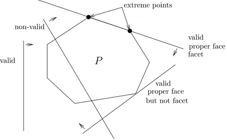
An inequality ax ≤ α is valid for a polyhedron P ⊆ Rn _{if for every solution x ∈ P ,}

ax ≤ α. This inequality is said to be tight for a solution x ∈ P if ax = α. The inequality ax ≤ α is violated by x ∈ P if ax > α. Let ax ≤ α be a valid inequality for the polyhedron P . F = {x ∈ P |ax = α} is called a face of P . We also say that F is a face induced by ax ≤ α. If F 6= ∅ and F 6= P , we say that F is a proper face of P . If F is a proper face and dim(F ) = dim(P ) − 1 , then F is called a facet of P . We also say that ax ≤ α induces a facet of P or is a facet defining inequality.

If P is full dimensional, then ax ≤ α is a facet of P if and only if F is a proper face and there exists a facet of P induced by bx ≤ β and a scalar ρ 6= 0 such that F ⊆ {x ∈ P |bx = β} and b = ρa.

If P is not full dimensional, then ax ≤ α is a facet of P if and only if F is a proper face and there exists a facet of P induced by bx ≤ β, a scalar ρ 6= 0 and λ ∈ Rq×n

(where q is the number of lines of matrix A=_{) such that F ⊆ {x ∈ P |bx = β} and}

b = ρa + λA=_.

An inequality ax ≤ α is essential if it defines a facet of P . It is redundant if the system A′_{x ≤ b}′_{} obtained by removing this inequality from Ax ≤ b defines the same}

polyhedron P . This is the case when ax ≤ α can be written as a linear combination of inequalities of the system A′_{x ≤ b}′_{. A complete minimal linear description of a}

polyhedron consists of the system given by its facet defining inequalities and its implicit equalities.

A solution is an extreme point of a polyhedron P if and only if it cannot be written as the convex combination of two different solutions of P . It is equivalent to say that x induces a face of dimension 0. The polyhedron P can also be described by its extreme points. In fact, every solution of P can be written as a convex combination of some extreme points of P .

Figure 1.3 illustrates the main definitions given is this section.

Consider a combinatorial optimization problem P. Let E be its basic set, c(.) the weight function associated with its variables and S the set of its feasible solutions. Suppose that P consists in finding an element of S whose weight is maximum. The problem P can be hence written as max{cx|x ∈ S}. If F ⊆ E, then the 0-1 vector xF _∈_RE _{such that x}F_{(e) = 1 if e ∈ F and x}F_{(e) = 0 otherwise, is called the incidence}

(23)

extreme points proper face facet valid proper face valid non-valid valid

P

but not facet

Figure 1.3: Valid inequality, facet and extreme points

the solutions of P or polyhedron associated with P. P is thus equivalent to the linear program max{cx|x ∈ P (S)}. Notice that the polyhedron P (S) can be described by a set of a facet defining inequalities. And when all the inequalities of this set are known, then solving P is equivalent to the resolution of a linear program.

Recall that the objective of the polyhedral approach for combinatorial optimization problems is to reduce the resolution of P to that of a linear program. Generally, it is difficult to characterize a polyhedron of a combinatorial optimization problem by a system of linear inequalities. In particular, when the problem is NP-hard there is a very little hope to find such a characterization. In addition, the number of inequalities describing this polyhedron is in general exponential. Therefore, even if we know the complete description of that polyhedron, its resolution remains in practice a hard task because of the large number of inequalities.

Fortunately, a technique called the cutting plane method can be used to overcome this difficulty. This method is described in what follows.

1.3.2 Cutting plane method

The cutting plane method is based on a crucial result in combinatorial optimization saying that only a partial description of the polyhedron can be sufficient to solve the problem optimally.

(24)

the difficulty of solving a linear program does not depend on the number of inequalities of that program, but on the separation problem associated with the inequality system of the program. Consider a polyhedron P in Rn _{and let Ax ≤ b be its system of}

inequalities. The separation problem associated with P consists in checking if the point x ∈ Rn _{satisfies all the inequalities Ax ≤ b and, if not, to find an inequality}

ax ≤ α of Ax ≤ b violated by x (see Figure 1.4).

Gr¨otschel, Lov´asz and Schrijver [67] prove that an optimization problem (for instance max{cx, Ax ≤ b}) can be solved in polynomial time if and only if the separation problem associated with Ax ≤ b is polynomial as well. This equivalence has permitted an important development of the polyhedral methods in general and the cutting plane method in particular.

x∗

P

ax≥ α

Figure 1.4: A hyperplan separating x∗ _{and P}

More precisely, the cutting plane method consists in solving successive linear pro-grams, with possibly a large number of inequalities, by using the following steps. Let LP = max{cx, Ax ≤ b} be a linear program and LP′ _{a linear program obtained by}

considering a small number of inequalities among Ax ≤ b. Let x∗ _{be the optimal}

so-lution of the latter. We solve the separation problem associated with Ax ≤ b and x∗. This phase is called the separation phase. If every inequality of Ax ≤ b is satisfied by x∗_{, then x}∗ _{is also optimal for LP . If not, let ax ≤ α be an inequality violated by x}∗_.

Then we add ax ≤ α to LP′ _{and repeat this process until an optimal solution is found.}

Algorithm 1summarizes the different cutting plane steps.

Note that at the end, a cutting-plane algorithm may not succeed in providing an optimal solution for the underlying combinatorial optimization problem. In this case a Branch-and-Bound algorithm can be used to achieve the resolution of the problem, yielding to the so-called Branch-and-Cut algorithm.

(25)

Algorithm 1: A cutting plane algorithm

Data: A linear program LP and its system of inequalities Ax ≤ b Result: Optimal solution x∗ _{of LP}

Consider a linear program LP′ _{with a small number of inequalities of LP ;} 1

Solve LP′ _{and let x}∗ _{be an optimal solution;} 2

Solve the separation problem associated with Ax ≤ b and x∗_; 3

if an inequality ax ≤ α of LP is violated by x∗ _then 4 Add ax ≤ α to LP′_; 5 Repeat step 2 ; 6 else 7 x∗ _{is optimal for LP ;} 8 return x∗_; 9

1.3.3 Branch-and-Cut algorithm

The Branch-and-Cut method, is a combination of the Branch-and-Bound and cutting-plane methods. The basic idea of branch-and-cut is simple. In each iteration, one solves a linear relaxation of the problem using a cutting plane algorithm. New valid inequalities are then added at each iteration to the current linear program. This permits to obtain increasingly better upper bounds on the value of the optimal solution of the combinatorial optimization problem. Branching occurs only when no violated inequalities are found to cut off infeasible solutions.

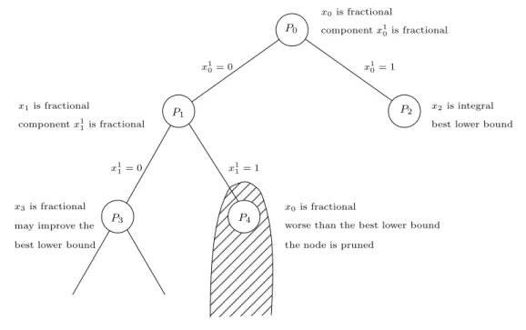
Consider again the combinatorial problem P defined above and assume now that its variables are binary. The polyhedron P (S) is often not completely known because P _{may be NP -hard. In this case, it would not be possible to solve P as a linear} program and in general, the solution obtained from the linear relaxation of P (S) is fractional. The resolution of P can then be done by combining the cutting plane method with a Branch-and-Bound algorithm. Such an algorithm is called a Branch-and-Cut algorithm. Each node of the Branch-and-Bound tree (also called Branch-and-Cut tree) corresponds to a linear program solved by the cutting plane method.

Suppose that P is equivalent to max{cx|Ax ≤ b, x ∈ {0, 1}n_{} and that Ax ≤ b has a}

large number of inequalities. A and-Cut algorithm starts by creating a Branch-and-Bound tree whose root node corresponds to a linear program LP0 = max{cx|A0x ≤

b0, x ∈Rn}, where A0x ≤ b0is subsystem of Ax ≤ b with a small number of inequalities.

Then, we solve the linear relaxation of P that is LR = max{cx|Ax ≤ b, x ∈Rn_{}, using}

(26)

be the optimal solution of LP0 and A′0x ≤ b′0 the set of inequalities added to LP0 at

the end of the cutting plane phase. If x∗

0 is integral, then it is optimal for P. If x∗0 is

fractional, then we start the branching phase. This consists in choosing a variable, say x1

0, having a fractional value and adding two nodes P1 and P2 in the Branch-and-cut

tree. The nodes P1 and P2 correspond to the linear programs LP1 = max{cx|A0x ≤

b0, A′0x ≤ b′0, x10 = 0, x ∈Rn} and LP2 = max{cx|A0x ≤ b0, A′0x ≤ b′0, x10 = 1, x ∈Rn},

respectively. We solve the linear program LR1 = max{cx|Ax ≤ b, x10 = 0, x ∈ Rn}

(resp. LR2 = max{cx|Ax ≤ b, x10 = 1, x ∈ Rn}) by a cutting plane method starting

from LP1 (LP2). If the optimal solution of LR1 (resp. LR2) is integral then, it is

feasible for P. Its value is thus a lower bound of the optimal solution of P and the node P1 (resp. P2) becomes a leaf of the Branch-and-Cut tree. If this solution is fractional,

then we select a variable with a fractional value and add two children to node P1 (resp.

P2), and so on.

Remark that at some node of the Branch-and-Cut tree, the addition of a constraint xi _{= 0 or x}i _{= 1 may make the associated linear program infeasible. Also, even if the}

corresponding linear program is feasible, its optimal solution may be worse than the best known lower bound of the tree. In both cases, we proceed the pruning phase and that node is cut off from the Branch-and-Cut tree. The algorithm ends when all the nodes have been explored and all the leaves of the tree are pruned. At the end of the algorithm, the optimal solution of P is the best feasible solution among the solutions obtained along the Branch-and-Bound tree.

Figure1.5illustrates a Branch-and-Cut tree. That is a Branch-and-Bound tree where in each node P i, i = 1, . . . , 4, a cutting plane method is used to solve the linear relax-ation of node Pi.

The polyhedral approach and in particular the Branch-and-Cut method have been successfully applied to several combinatorial optimization problem that are considered difficult to solve, such as the Travelling Salesman Problem [8], the Max-Cut prob-lem [21] and the Survivable Network Design Problem [86]. The efficiency of this approach depends on two important theoretical and practical issues. The first one consists in determining a good partial description of the convex hull of the solutions of the problem in terms of linear inequalities. The second issue is to devise efficient separation algorithms (exact or heuristic) for the identified classes of inequalities.

Note that the cutting plane method is effective when the number of variables is polynomial. However, when the number of variables is huge (for example exponential), one should resort to other appropriate methods such as the column generation method that we describe briefly in the following section.

(27)

00000

11111

P1 P3 x1 0= 0 x 1 0= 1 x11= 0 x 1 1= 1 component x1 0is fractional x0is fractional x3is fractional

may improve the best lower bound

component x11is fractional

x1is fractional x2is integral

best lower bound

x0is fractional

worse than the best lower bound the node is pruned

P0

P2

P4

Figure 1.5: A Branch-and-Cut tree

1.4 Column generation and Branch-and-Price

There are several reasons that motivate the MIP formulations using a huge number of variables. Indeed, generally a compact formulation of a MIP have a weak LP relaxation, which can be tightened by a reformulation that involves a huge number of variables. Moreover, in some cases, a compact formulation of a MIP may have a symmetric structure which causes a poor performance of the branch-and-bound since the problem barely changes after branching. Consequently, a reformulation with a huge number of variables can eliminate this symmetry.

To solve such large-scale problems, the technique widely applied is the one called column generation method.

1.4.1 Column generation method

This method is used to efficiently solve linear programs with an exponential number of variables by considering only a small number of them. The method appears in the 1960’s to solve problems related to huge data that could not be stored in the computers at this time. Dantzig and Wolfe [36] were the first to introduce this technique in their decomposition method. The Dantzig-Wolfe decomposition is a reformulation approach

(28)

that is based on is a special form of variable redefinition. It can be represented using the concept of generating sets: for each sub-system on which the decomposition is based, one defines a finite set of generators from which each subproblem solution can be generated. The variables of the reformulation shall be the weights of the elements of these generating sets (more details concerning the Dantzig-Wolfe decomposition can be found in [132]). The column generation technique can be also used to deal with problems having a large number of variables. In this optic, Gilmore and Gomory [58,59] used this approach for the cutting stock problem.

The general idea is that optimal solutions to large LP’s can be obtained without explicitly including all columns in the constraint matrix. In fact, only a subset of all columns will be in the optimal solution and all other (non-basic) columns can be ignored. The idea of a column generation algorithm is to solve a sequence of linear programs having a reasonable number of variables (also called columns). The algorithm starts by solving a linear program having a small number of variables and which forms a feasible basis for the original program. At each iteration of the algorithm, we solve the so-called pricing problem whose objective is to determine the variables which must enter the current basis. These variables are those having a negative reduced cost (for a ”minimize” objective function). The reduced cost associated with a variable is computed using the dual variables. We then solve the linear program obtained by adding these variables and repeat the procedure. The algorithm stops when the pricing algorithm does not generate new columns to add to the current basis. In this case, the solution obtained from the last restricted program is optimal for the original one. When the pricing problem is NP-hard, one can use some appropriate heuristic procedure to solve it. However, at the last iteration, it must be solved by an exact method to prove the optimality of the solution. Notice that the column generation method can be seen as the dual of the cutting plane method as it adds columns (variables) instead of rows (inequalities) in the linear program. For more details on the column generation method, the reader is referred to [94, 130, 38].

1.4.2 Branch-and-Price algorithm

In order to solve integer linear programs, the column generation method can be com-bined with a and-Bound algorithm. The obtained algorithm is called a Branch-and-Price algorithm. The principle of and-price is similar to that of branch-and-cut except that the procedure focuses on column generation rather than row gener-ation. Similarly to the Branch-and-Cut algorithm, the branching phase happens when no columns price out to enter the basis and the solution given by the linear program

(29)

Algorithm 2: A column generation algorithm

Data: A linear program MP (Master Problem) with a huge number of variables Result: Optimal solution x∗ of MP

Consider a linear program RMP (Restricted Master Problem) including only a

1

small subset of variables of the MP ;

Solve RMP and let x∗ _{be an optimal solution;} 2

Solve the pricing problem associated with the dual variables obtained by the

3

resolution of the RMP;

Denote C = {x| reduced cost (x) < 0}, the set of variables (columns) with a

4

negative reduced cost; if C 6= ∅ then

5

Add the variables of C to RMP ;

6 Repeat step 2 ; 7 else 8 x∗ _{is optimal for LP ;} 9 return x∗_; 10 is yet fractional.

In the literature, the Branch-and-Price algorithm has been extensively used to solve large scale problems such that the cutting stock problem [6], the integer multi-commodity flow problem [18], the crew scheduling problem [129], etc...

Moreover, it is possible to combine both column and row generation. This combina-tion is very interesting since it can yield very strong LP relaxacombina-tions. However, dealing with the two generation processes is not trivial. The main difficulty is, after additional rows are added, the structure of the pricing problem can be destroyed and its resolution becomes much harder.

Despite these difficulties, there have been some successful applications of combined row and column generation (see for example [17]).

1.4.3 Primal heuristics

The Branch-and-Price (resp. Branch-and-Cut) algorithm can be improved by deriving good primal feasible solutions to the combinatorial optimization problem. This can be achieved using the so-called primal heuristics, which compute good lower bounds

(30)

that can be used to prune suboptimal branches of the Branch-and-Price tree (resp. Branch-and-Cut tree).

Primal heuristics can be used at the root to find early a first feasible solution. They also may be used at a given node of the tree mainly to round fractional solutions and try to get a better bound. As a consequence, they help reducing considerably the number of generated nodes of the tree as well as the CPU time. Moreover, this guarantees to have an approximation of the optimal solution of the problem for example when a CPU time limit has been reached.

1.5 Extended Formulations

To formulate a Combinatorial Optimization Problem P, the natural way is to define an integer variable xe for each e ∈ E and find a suitable set of constraints to represent

F_{. Recall that E represents the basic set of P and F is a family of subsets of E. A} formulation using only variables xe is called natural formulation, and can be written

as follows.

Min X

e∈E

c(e)xe

s.t. Ax ≥ b (1.1)

xe integer for all e ∈ E. (1.2)

Although a natural formulation is a direct formulation using generally a reasonable number of variables, it can present some drawbacks. In fact, without adding valid inequalities, natural formulations usually have a loose linear relaxation. As a con-sequence, to improve natural formulations one should resort to new classes of valid inequalities defining in preference facets. This may imply separation procedures that can be heavy to compute, mainly when the associated separation problem is NP-hard. Moreover, natural formulations often have a number of constraints that is exponential in the size of the problem.

An attractive alternative to overcome these drawbacks is to introduce additional variables, and thus work in a higher dimensional space. The resulting formulation is called extended formulation. In what follows, we give some preliminary notions about extended formulations. For more details, the reader is referred to [128, 29].

We distinguish exact and compact extended formulation. By exact, we mean that the projection onto the original space of variables gives the convex hull of the solutions in

(31)

this space. This implies that the value of the dual bound is equivalent to that obtained when carrying out separation over the convex hull of the solutions. Also by compact, we mean that the number of variables and constraints of the extended formulation is polynomial in the size of the problem. Hence, theoretically, adding a priori such an extended formulation to tighten a mixed-integer model provides an alternative to the separation.

An extended formulation can be defined with respect to a given original formulation (a natural formulation or an already extended one) as follows. Suppose that there are n original variables x and p extended variables y. Suppose there are m constraints, that may involve only x variables, only y variables, or both sets of variables. We also assume that the cost function and the integrality requirements are only on the x variables, which is reasonable, because the original formulation could do that.

Min X

e∈E

c(e)xe

s.t. Ax + By ≥ b (1.3)

x integer. (1.4)

An extended formulation can be compared with a formulation on the original vari-ables by projecting its associated polyhedra onto the x space. Let Q = {(x, y) ∈ Rn_Rp _:

Ax + By >= b}. The projection of Q onto x is defined as projx(Q) = {x ∈ Rn : ∃y ∈

Rp_{, Ax + By >= b}.}

The use of extended formulations have many potential advantages. In fact, as mentioned above, extended formulations have the potential for providing high-quality bounds on some combinatorial optimization problems where the natural formulations perform poorly. In addition, some very complex families of facet-defining inequalities on the natural variables can be obtained by the projection of quite simple inequalities on the extended variables. Moreover, an inequality on the natural variables, even when facet-defining, can generally be lifted when expressed in the extended space of variables. Furthermore, when the separation of a certain family of inequalities in the original vari-ables is NP-hard, a superfamily of valid inequalities obtained by a projection from an extended formulation can be separated in polynomial time.

However, extended formulations may present some drawbacks. First, because for some combinatorial optimization problems, stronger extended formulations are signif-icantly huge as using a large number of variables. Moreover, sometimes the linear programs of large extended formulations can be highly degenerate, mainly when using the simplex algorithm to solve the linear relaxation.

(32)

1.6 Graph theory: definitions and notations

In this section, we present some basic definitions and notations of graph theory that will be necessary for the subsequent chapters. For more details, the reader is referred to [123].

The graphs we consider are either directed or undirected, finite, loopless and without multiple edge or arcs.

An undirected graph is denoted by G = (V, E) where V is the set of nodes and E is the set of edges. If e ∈ E is an edge with endnodes u and v, we also write uv to denote e. Given W and W′_{, two disjoint subsets of V , [W, W}′_{] denotes the set of edges of G}

having one endnode in W and the other in w′_{. If W}′ _{= W , then [W, W ] is called a cut}

of G denoted by δ(W ) (see Figure 1.6). For a node subset W ⊆ V and a node v ∈ V , we write [v, W′_{] for [{v}, W}′_{] and we denote by W the node set V \ W .}

W V\W

δ(W )

Figure 1.6: A cut δ(W )

If Π = (V1, . . . , Vp), p ≥ 2, is a partition of V , then we denote ∆ = δ(Π) the set

of edges having their endnodes in different sets. We may also write δ(V1, . . . , Vp) for

δ(Π). Note that for W ⊂ V , δ(W ) = δ(W, W ). If s and t are two nodes of G such that s ∈ W and t ∈ W , then δ(W ) is called st-cut of G.

A directed graph is denoted by D = (V, A) where V is the node set and A the arc set. An arc a with origin u and destination v is denotes by (u, v). Given two node subsets W and W′ _{of V , [W, W}′_{] denotes the set of arcs whose origins are in W and}

destinations in W′_{. As before, we write [u, W}′_{] for [{u}, W}′_{] and W denotes the node}

set U \ W . The set of arcs having their origins in W and destinations in W is called a directed cut or dicut of D. This arc set is denoted either by δ+_{(W ) or δ}−_{(W ). We also}

write δ+_{(u) for δ}+_{({u}) and δ}−_{(u) for δ}−_{({u}) with u ∈ U. If s and t are two nodes of}

(33)

Let G′ _{= (V}′_{, E}′_{) (resp. D}′ _{= (V}′_{, A}′_{)) with V}′ _{⊆ V and E}′ _{⊆ E (resp. V}′ _{⊆ V and}

A′ _{⊆ A) be a subgraph of G (resp. D). If c(.) is a weight function which associates}

with an edge (resp. arc) e ∈ E (resp. a ∈ A) the weight c(e) (resp. c(a)), then the total weight of G′ _{(resp. D}′_{) is c(E}′_{) =} P

e∈E′

c(e) (resp. c(A′_{) =} P

a∈A′

c(a)).

In the notations, we will specify the graph as a subscript (that is, we will write δG(W ),

δG(Π), δG(V1, . . . , Vp), δD+(W ), δ −

D(W ), [W, W′]G, [W, W′]D) whenever the considered

graphs may not be clearly deduced from the context.

Given an undirected graph G = (V, E), for all F ⊆ E, V (F ) will denote the set of nodes incident to the edges of F . For W ⊂ V , we denote by E(W ) the set of edges of G having both endnodes in W and G[W ] the subgraph induced by W , that is the graph (W, E(W )). Given an edge e = uv ∈ E, contracting e consists in deleting e, identifying the nodes u and v and in preserving all adjacencies. Contracting a node subset W consists in identifying all the nodes of W and preserving the adjacencies. Given a partition Π = (V1, . . . , Vp), p ≥ 2, we will denote by GΠ the subgraph induced

by Π, that is, the graph obtained from G by contracting the sets Vi, for i = 1, . . . , p.

Note that the edge set of GΠ is the set δ(V1, . . . , Vp).

A path P of an undirected graph G is an alternate sequence of nodes and edges (u1, e1, u2, . . . , ul−1, el, ul) where ei = [ui, ui+1] for i = 1, . . . , l − 1. We will denote a

path P either by its node sequence (u1, . . . , ul) or its edge sequence (e1, . . . , el−1). The

nodes u1 and ul are called the endnodes of P , while its other nodes are said to be

internal. A path is simple if it does not contain the same node twice. In the sequel, we will always consider that the paths are simple. By opposition, a non-simple path is called a walk. A path whose endnodes are s and t will be called an st-path. A cycle in G is a path whose endnodes coincide, that is u1 = ul. Also, a cycle is simple if it does

not contain twice the same node, excepted u1. We call a chord an edge between two

non-adjacent nodes of a path.

Similarly, we call a dipath P a path in a directed graph, that is an alternate sequence of arcs (u1, a1, u2, . . . , ul−1, al, ul) with ai = [ui, ui+1] for i = 1, . . . , l − 1. A dipath is

denoted either by its node sequence (u1, . . . , ul) or its arc sequence (a1, . . . , al−1), and

the nodes u1, ul are called the endnodes of that dipath. A dipath whose endnodes

coincide (u1 = ul) is called a circuit. If u1 = s and ul = t then P is called an st-dipath.

A dipath is simple if it does not contain twice the same node.

An undirected (resp. directed) graph is said connected if for every pair of nodes (u, v) there exists at least one path (resp. dipath) between u and v. A connected graph which have no cycle (resp. circuit) is called tree. A connected component of a graph G (resp.

(34)

D) which is maximal, that is adding a node or an edge (resp. arc) to that subgraph gives a non-connected graph.

Given an undirected (resp. directed) graph G = (V, E) (resp. D = (V, A)), two st-paths (resp. st-dipaths) are said to be edge-disjoint (resp. arc-disjoint) if they have no edge (resp. arc) in common. They are node-disjoint if they have no internal node in common. A graph is said to be k-edge-connected (resp. k-arc-connected ) if it contains at least k edge-disjoint (resp. arc-disjoint) st-paths (resp. st-dipaths) for all pair of node {s, t} ∈ V × V (resp. {s, t} ∈ V × V ).

Given an undirected graph G = (V, E), a demand set K ⊆ V × V is a subset of pairs of nodes, called demands. For a demand {O, D} ∈ K, O is the origin and D is the destination of that demand. A node involved in a path P routing a demand k will be called a terminal for that demand, while the other nodes are rather Steiner nodes for the considered demand.

A complete graph is a graph in which there is an edge between each pair of nodes. A complete graph with n nodes is denoted by Kn.

An undirected graph is outerplanar when it can be drawn in the plane as a cycle with non crossing cords.

A graph is series-parallel if it can be obtained from a single edge by iterative appli-cation of the two operations: addition of a parallel edge, subdivision of an edge.

Observe that a graph if series-parallel if and only if it is not contractible to K4.

Similarly, a graph is outerplanar if and only if it is not contractible to K4 and K3,2.

Therefore, an outerplanar graph is also series-parallel.

A graph G is said to be Halin graph if G = (C ∪ T, E) where the subgraph of G induced by T is a tree whose leaves forms the cycle C in G.

(35)

Multilayer telecommunication

networks

2.3.2 Multilayer survivable network design . . . 42 Nowadays, telecommunication networks provide a large variety of services enabling the transport of different kind of data such as vocal messages, photos, videos, etc. In addition to this variety, exchanged data have witnessed an explosive growth due mainly to the fast development of Internet. As a consequence, telecommunication networks have been evolving towards a multilayer architecture, which has proved to be the most powerful and the most adapted to all these changes and improvements. Moreover, as

(36)

these networks are involved in the transportation of important data for companies, ad-ministrations and governments, they ought to be sufficiently survivable, so that network services can be restored in the event of a catastrophic failure.

In this chapter, we give a brief idea about the functionalities of multilayer networks. We first present the multilayer structure in telecommunication networks and focus es-pecially on the IP-over-WDM model. More precisely, we present the particularities of the IP and WDM layers and discuss the technologies corresponding to each one. Then, we show the different ways of interaction between the two layers and present in particu-lar the GMPLS technology. We further introduce some concepts related to survivability in general and to its application in the multilayer context. We finish the chapter by a quick survey on multilayer network design problems and in particular the ones dealing with survivability issues.

2.1 Telecommunication networks: toward a

multi-layer structure

2.1.1 Evolution of networks’ architecture

Figure 2.1: Reference Model OSI

For historical reasons, telecommunication networks have been represented as the superposition of several technological layers. Using the bottom technology, each layer has a specific functionality that provides a service for the layer above. Moreover, each layer is characterized by appropriate protocols. A protocol can be defined as a formal

(37)

description of the conventions and rules that are used by a layer to manage data traffic and govern the interactions with the other layers. In order to classify the different protocols, the ISO (International Standardization Organization) proposed a seven-layer model known as the OSI (Open Systems Interconnection) model (see Figure 2.1).

Although the OSI model constitutes a reference that helped to well understand the multilayer network process, it remains significant only from a theoretical point of view. In reality, one should expect to have less than seven layers such that each layer can ensure several functions at a time.

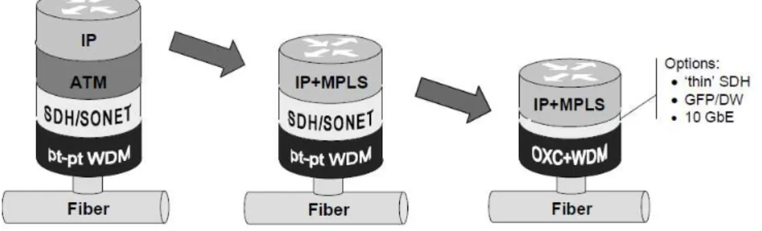
In a further classification, the network has been represented using IP routers over ATM switches over SDH network components. The IP (Internet Protocol) layer is used as a platform for users’ applications, ATM (Asynchronous Transfer Mode) for traffic engineering, flow control and QoS (Quality of Service) support, and SDH (Synchronous Digital Hierarchy) for the transportation of ATM flows over WDM optical network (Wavelength Division Multiplexing) [57] (see Figure 2.2).

Figure 2.2: Evolution towards the IP-over-WDM model

Again, the resulting architecture creates more complications rather that simplifying the network. Due to the number of layers involved, this architecture stacks redundant functionalities and presents many operational complexities. In fact, when delivering data, each layer adds heavy control information (for encapsulation), yielding to an over-cost bandwidth and a very complex data processing over the nodes. Furthermore, this four-layer architecture shows a great lack of flexibility that impedes it to cope with the continuous increase of data traffic [93]. Moving towards a more flexible, dynamic and cost-effective architecture was consequently necessary.

The most straightforward alternative was to bypass all intermediate layer technologies and implement the IP directly over WDM, hence resulting in a simple two layer model, referred to as IP-over-WDM [93, 124].

(38)

The IP-over-WDM model presents many advantages. In fact, WDM technology can manage the continuous growth of traffic using the already existing infrastructure. This is thanks to the huge capacities of optical fibres which may ensure the transportation of many terabits per second. Moreover, since telecommunication operators choose to put all the different types of traffic (voice, data and video) on a single physical medium, the majority of traffic has become of type IP.

Nevertheless, the implementation of this new two layer model has been a bit challeng-ing. In fact, the deleted intermediate layers provide important functionalities, such as traffic engineering in ATM or multiplexing and fast protection in SDH. Moving to the two layers IP-over-WDM model, these functionalities had to be continuously ensured by moving them either down to the optical layer, or up to the IP layer.

To overcome this difficulty, telecommunication operators had the idea of using the control protocols such as the MPLS (Multi-Protocol Label Switching) and the GMPLS (Generalized-MPLS) [115, 100]. These protocols permit the implementation of the traffic engineering in the IP layer (at the packet level) and in the optical layer (at the wavelength level), and hence the ATM can be removed from the network. Similarly, many functions of the SDH can be moved down to the optical layer, enhanced with optical switching capabilities and supported by advanced control mechanisms, now referred to as the OTN (Optical Transport Network) [134].

2.1.2 The IP layer

The role of the Internet layer is to ensure the interoperability and interconnection between the different AS (Autonomous System) subnetworks constituting it, allowing thus data to be routed through these networks until destination. To this end, it uses the IP protocol which is responsible of data routing.

2.1.2.1 IP Protocol

To be routed in the network, the data is divided into IP packets. An IP packet is composed of two parts: a header having information for various transport, in particular the destination IP address, and a data portion. The Internet Protocol (IP) [48, 81,

108] manages the transmission of these packets called datagrams through a set of interconnected networks from a source to a destination. The source and destination are host machines (terminals) identified by fixed length addresses called IP address. Many other protocols such as the TCP (Transmission Control Protocol) are used to

(39)

complete the packet headers in order to ensure a correct packets’ routing and a rapid detection of errors [109].

2.1.2.2 Traffic routing

Traffic routing is one of the main functions of the Internet layer. The routing consists in determining a path in order to connect two distant terminals. Determining a path is a complex task that is performed in large networks using dedicated protocols. The role of these protocols is to discover the network topology and derive the best route. There are several routing protocols that differs in the criteria of choosing routes and the accuracy of the topology discovery. We distinguish for example, the RIP (Routing Information Protocol) that allows each router to know the distance separating the other routers from the IP network in term of hops. There is also the OSPF (Open Shortest Path First) protocol, which, being more efficient than RIP, has gradually replaced it. In fact, unlike RIP, the OSPF sends to all the adjacent routers the number of hops that separates them from the IP networks. Then, each router transmits to all the routers in the network the status of each of its links. A third protocol is the so-called IS-IS (Intermediate System to Intermediate System). The IS-IS is a link-state protocol that enables routers to have maintain a common view of network’s topology. Each router makes its own topological database and then shared among the remaining routers. Packets are then transmitted via the shortest path. Finally, we can mention the BGP (Border Gateway Protocol) that is used to convey large volumes of data through the network.

The majority of routing protocols rely on traditional algorithms calculating shortest paths in the network. However, they do not generally take into account other crite-ria such as delays or congestion, which can degrade seriously the performance of the network. In this optic, telecommunication operators have been always seeking a good and optimal way to manage their networks. In particular, in order to ensure a better routing procedure, they thought of the introduction of the MPLS system, that will be presented in the next section.

2.1.2.3 MPLS technology

In traditional IP networks, packets’ routing is performed using the destination address contained in the header of the IP layer’s packet. To decide which is the next hop, each router of the IP layer consults its routing table and determines the outgoing interface to which the packet will be sent. Generally, the mechanism of research in the routing

(40)

table is time consuming. Moreover, with the growth of the networks’ size in the recent years, the routing tables’ size has been steadily increasing, making it necessary to find a more efficient method to route packets. Telecommunication operators have then opted for the MPLS (Multi Protocol Label Switching) technology.

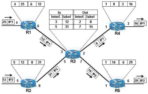
MPLS is a multilayer switching system that was inspired from Tag Switching nologies of Cisco and also from the ARIS (Aggregate Route-Based IP Switching) tech-nology of IBM. MPLS was designed to improve the efficiency of routers in packet processing. Indeed, instead of being analysed at each router, the packets are analysed only once at the entrance of the network, and then routed along a path thanks to a system of labels. As its name indicates, MPLS is based on the technique of label switching. Figure 2.3 illustrates this mechanism. For example, an IP packet entering to the router R3 through the interface 5, with the label 31 will after be sent to the router R5 using interface 7 and the outgoing packet will be labeled 14 instead of 31. Note here that the forwarding table of labels has far fewer entries than the usual IP routing table. The switching procedure is hence done by routers that do not need to consult the IP address or the routing table. These routers are called LSR (Label Switch Routers).

Figure 2.3: An example of label switching

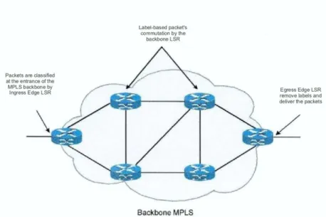
The LSR use the labels to switch packets inside the MPLS network (see Figure2.4). MPLS routers at the periphery of the network are called Edge LSR. These routers have both traditional and IP interfaces connected to the MPLS network, and are

(41)

re-sponsible for imposing or removing labels on IP packets that pass through them. In particular, the Edge LSR can be divided into two classes: the Ingress LSR (ingress routers) responsible for imposing labels to IP packets that pass through to enter the MPLS backbone, and the Egress LSR (egress routers) that remove the added labels.

Figure 2.4: LSR

When the packets enter the the MPLS network, Ingress LSR classify them into different classes called FEC (Forwarding Equivalent Classes). These classes can be formed according to several criteria such as the same prefix as the destination address for the IP routing, packets of the same application, packets from the same source address prefix, the quality of service required, etc. Hoewever, in general FEC are defined in terms of IP prefixes that are given by the IGP (Interior Gateway Protocol), and the information related to the quality of service insured by the so-called TE (Traffic Engineering). After the classification step, packets belonging to the same FEC will follow the same path and will be managed by the same method of forwarding. In fact, once inside the MPLS network, the packets can never be reclassified. The succession of LSR that have been used by an FEC constitutes the so-called LSP (Label Switched Path), also said the labels’ switching path. This path is always unidirectional and unique for each FEC.

Originally, MPLS was developed for fast packet switching, but it has quickly allowed the implementation of higher level solutions such as VPN (Virtual Private Networks). This will be explained in details in the next section.

(42)

2.1.2.4 Virtual Private Network

A virtual private network (VPN) can be seen as an extension of an organisation private network in order to connect remote users over shared or public network. A private network is one where all data paths are secret to a certain extent, yet open to a limited group of persons. A VPN allows, for example, to interconnect networks of the same company in multiple locations.

VPNs are IP-based networks that use encryption and tunnelling to achieve the fol-lowing goals:

• connect users securely to their own corporate network (remote access), • link branch offices to an enterprise network (intranet),

• extend organizations’ existing computing infrastructure to include partners, sup-pliers and customers (extranet).

VPNs often use the MPLS technology to connect sites belonging to one or more VPN since the MPLS LSP tunnels provide a good medium for the encapsulation of VPN traffic. These networks are called MPLS-VPN.

Figure 2.5: Different types of routers in an MPLS-VPN In an MPLS-VPN, we distinguish several types of routers (see Figure 2.5):